Discrete-Time System Conditional Optimization Based on Takagi–Sugeno Fuzzy Model Using the Full Transfer Function

Abstract

The study proposes a novel method for synthesis of a discrete-time parallel distributed compensation (PDC) controller for the nonlinear discrete-time Takagi–Sugeno (TS) fuzzy plant model. For each of the fuzzy plant model linear subsystems, a local linear first order proportional-sum (PS) controller is designed. The algebraic technique is used in two-dimensional parameter space, utilizing the characteristic polynomial of the row nondegenerate full transfer function matrix. Each system’s relative stability is accomplished in relation to the selected damping coefficient. The supplementary criterion is the minimal value of the performance index in the form of the sum of squared errors (SSE). However, unlike the traditional technique, output error is influenced by all simultaneous actions on the system: nonzero inputs and nonzero initial conditions. The full transfer function matrix of the system allows for the treatment of simultaneous actions of the input vector and unknown unpredictable initial conditions. In order to show the improvement caused by the application of a new optimization method that considers nonzero initial conditions, a comparison of PDC controllers designed under zero and nonzero initial conditions is given, where the system in both cases starts from the same nonzero initial conditions, which is often the case in practice. The simulation and experimental results on a DC servo motor are shown to demonstrate the suggested method efficiency.

1. Introduction

Dynamic systems are affected simultaneously by the initial conditions and the input vector. There is no physical or mathematical reason to ignore the initial conditions in control optimization. Papers [1,2] provide a novel way to design traditional proportional–difference–sum (PDS) type controllers for a linear mathematical model of a plant in a closed-loop control system. Using the notion of the full transfer function matrix, a new conditional optimization approach in the parameter space of two adjustable parameters is proposed. The use of the full transfer function matrix enables the introduction of a new type of performance index—the sum of squared errors that occurs in the most broad and realistic condition under all actions performed simultaneously on the system—nonzero initial conditions and nonzero inputs. Illustrative simulation and experimental results confirmed the following conclusion: the set of controller parameters that is optimal for the performance of the control system under all zero initial conditions is not optimal for its performance under nonzero initial conditions. This paper presents the continuation and application of a nonlinear discrete-time PDC control system to a nonlinear discrete-time TS fuzzy plant model.

In the field of analysis and application of proportional–integral–derivative (PID) type control algorithms, there is a great diversity in terms of papers and results. An overview of the situation is given in [3]. Just some of the examples are [4,5]. The solution of designing a discrete controller for a discrete plant is discussed in [4]. Paper [5] proposes a control parametrization-based optimum PID tuning technique for a single-link manipulator. The control system’s performance specifications are expressed as continuous state inequality constraints. The single-link manipulator’s PID optimum tuning issue may thus be framed as an optimal parameter selection problem with continuous inequality constraints. The constraint transcription approach, in conjunction with a local smoothing technique, handles these continuous inequality requirements. As a result, ref. [6] presents an optimum design strategy for the PID parameters in discrete-time systems for maximizing the reference tracking and disturbance rejection performances, respectively.

For every given linear time-invariant (LTI) plant, ref. [7] tackles the challenge of defining the set of all stable PID type controllers without parametric models. The frequency response data and the number of right-half-plane (RHP) poles of the plant are shown to be the only information needed for designing, and all stabilizing domains in the parameter space of PID-type controllers are determined by the boundaries, which are analytically described using the D-decomposition technique. Other research studies found a stability region in the parameter space as well. Authors accomplished it in the state space form for both discrete-time systems and also for continuous time in [8]. In the root signs invariant regions, researchers decomposed the area in the parameter plane for a continuous-time system in the state space form [9]. Kipnis and Nigmatulin [10] dealt with a trinomial discrete equation with two delays and offered a criterion for evaluating Lyapunov stability reliant on parameter values, as well as an extension of the Lyapunov stability theory via the new $r-$ stability concept. Gryazina et al. [11] outlined the state of the art for continuous-time system parameter synthesis beginning with Vishnegradsky and went over Neimark to the present, with latest additions and unique results that relate to the stability domain in the parameter space and considering the $H_{\infty }$ criterion, robustness, uncertainty and so on.

Plant control using the traditional control algorithm has been very relevant from the past to the present day, and researchers are actively experimenting with it. The DC servo motor is often the object of automatic control and has a very wide range of applications, which can be seen on the basis of the following works. Article [12] introduced deterministic artificial intelligence (D.A.I.) to control direct current motors used by unmanned underwater vehicles. Paper [13] describes how to regulate the speed of a permanent magnet direct current motor using a buck converter with Zero Average Dynamics. An analytic solution to state-constrained optimum tracking control issues for continuous-time linear time-invariant (CT-LTI) systems using model-based prediction, the quadratic penalty function and the variational technique is presented in [14]. As a result, study [15] describes how to control the speed of a DC motor using a buck converter controlled using zero average dynamics and fixed point induction control (ZAD-FPIC) methods. Proportional–integral, fuzzy and adaptive neuro fuzzy controllers were developed for a DC servo motor in [16]. In [17] different metaheuristic algorithms for creating PID controllers for DC motor are investigated, and these algorithms and classical methodologies are thoroughly compared in order to identify the optimum methodology for PID controller design and parameter tuning.

There are several applications of fuzzy logic that may be used for control reasons. Study [18] proposes a method for creating two-variable fuzzy logic controllers (FLCs). The equivalent relationship between a typical PID controller and a FLC was proposed and clearly identified in [19]. Furthermore, the analogous FLC designed in discrete form was presented and simulated, with system responses comparable to the original conventional PID controller.

Fuzzy control based on the Takagi–Sugeno fuzzy model is used in this study. Research and results in the application of Takagi–Sugeno type fuzzy systems in the tasks of modeling and control of dynamic systems are given in [20,21]. Review paper [22] gives an idea of past, present and future trends in the application of this type of system. Multiple articles on the TS discrete-time fuzzy models can be found in the literature, including [23,24,25]. The fuzzy model proposed by Takagi and Sugeno [26] is described by fuzzy IF–THEN rules, which depict local linear input–output relations of a nonlinear system. Paper [27] describes the construction of a fuzzy controller for the output–voltage regulation problem in switching converters based on a TS fuzzy model. Research [28] presents a unique method for constructing a TS fuzzy model of an unknown nonlinear system using experimental data. The observer-based fuzzy controller design technique for nonlinear discrete-time singular systems represented by TS fuzzy models is investigated in [29].

The second application of fuzzy systems, for example, is the PDC. In the work [30], a fuzzy controller is built using a PDC technique and applied in an experimental tank-level control system. In [31], a unique modification of the original PDC technique is proposed, such that, in addition to the stability issue, the system closed-loop performance may be addressed at the design stage. Initially, the nonlinearity can be successfully modeled by a number of local linear input–output connections. The observer-based fuzzy controller is then built using PDC technology and the proportional–derivative (PD) feedback scheme. Another study [32] provided a unified method for a nonlinear model following control that includes the regulation and servo control issues as specific examples.

An overview of some papers dealing with various optimizations follows below. The challenge of distributed controller design for linear discrete-time systems is discussed in [33]. The solution to optimum control issues for limited discrete-time linear hybrid systems based on quadratic or linear performance criteria is investigated in [34]. The paper has two objectives. The first is to provide some fundamental theoretical conclusions about the construction of the optimum state-feedback solution and the objective function. The second is to show how to combine multiparametric programming with dynamic programming to create the state-feedback optimum control law. A comparison of the linear and nonlinear controllers is given in [35]. More precisely, a robust pole-placement discrete time controller for a linearized uncertain polytopic model is compared to a nonlinear continuous-time control based on feedback linearization. The analytic solution to the Localized LQR (LLQR) optimum control challenge was developed in [36]. Paper [37] showed how an infeasible primal–dual interior point technique can be utilized to efficiently solve a robust optimum control problem with possible uses to model predictive control. The tasks of multicriteria optimization in controlling technological systems are reduced to multicriteria problems of fuzzy mathematical programming, and a heuristic algorithm for solving the formulated problem of optimal control is developed based on modifying the principles of maximin and Pareto optimality, [38]. In [39], a formulation of the problem of multicriteria optimization is obtained, considering the partial fuzziness of the starting information. A heuristic method for its solution is proposed, which is based on the experience of the decision maker.

Feldbaum in [40] was one of the first to study the transient response of linear systems with nonzero initial conditions. After that, study in this area diminished; thus, transient response referred to the system’s reaction under zero initial conditions and with a unit step function of the input. In [41], Izmailov proved that if the closed system’s poles are displaced far to the left in the complex plane, substantial deviations of the trajectory from the coordinate origin are unavoidable. In [42], Polyak et al. continue the work of Feldbaum and Izmailov on transient response in systems with nonzero initial conditions. This was accomplished by proposing a more precise estimate of the overshoot amplitude and demonstrating that large deviations produce effects for different pole locations. They also looked at determining the upper deviation limit using the linear matrix inequalities approach (LMI).

The theoretical basis for this research is, first of all, the concept of the full transfer function matrix defined for linear discrete systems, and then the TS type of fuzzy systems, with application in modeling, identification and control of dynamical systems. A full transfer function matrix, which was introduced and developed in [43,44,45], resolved controversy between the system transfer function and the stability testing using a classical transfer function. It is well understood that system stability, by definition, represents a dynamical attribute of the system in the free working regime for all zero input and variable arbitrary unknown initial conditions. The transfer function is defined for the system in the forced working regime under nonzero input and all zero initial conditions. This concept was applied in articles [1,2]. In these papers, the area of relative stability was derived, where the closed system has a predetermined damping coefficient. After that, conditional optimization was performed in the cases of proportional–difference–sum-type linear controllers with two and three adjustable parameters. A new performance index is presented that is entirely compatible with the use of the full transfer function matrix. The output error used in the performance index is influenced by all actions at the same time: by external inputs and by nonzero initial conditions.

Based on the conclusion that the optimal parameters obtained for zero are not optimal for nonzero initial conditions, in the case of linear discrete systems, it is intuitively imposed that something similar can also be valid in the case of nonlinear discrete systems. In order to apply the full transfer function (which, of course, applies to linear systems), the property that TS fuzzy systems can represent a class of nonlinear dynamical systems, composed of linear (or linearized) subsystems, is used. In this way, it is possible to use the full transfer function matrix, define new control algorithms, and determine the optimal parameters of the controller in the case of nonzero initial conditions. Compared with existing approaches, a new conditional optimization procedure based on the full transfer matrix is used in this paper. It allows the optimization procedure to be performed in the presence of the simultaneous action of both input and nonzero initial conditions.

2. Takagi–Sugeno Fuzzy Model

The TS fuzzy modeling method’s primary idea is to split nonlinear system dynamic behavior into numerous individually linearized systems, such that the entire nonlinear system behavior may be represented by fuzzy mixing of such systems. As a result, the fuzzy rule associated with the i-th linear system is specified as the i-th rule:

IF $z_1\left(k\right)$ is $M_{i1}$, and $z_2\left(k\right)$ is $M_{i2}$, ..., and $z_p\left(k\right)$ is $M_{ip}$ THEN

$$\begin{array}{cc}\hfill \mathbf{x}(k+1)& =A_i\mathbf{x}\left(k\right)+B_i\mathbf{u}\left(k\right),i=1,2,...,r,\hfill \\ \hfill \mathbf{y}\left(k\right)& =C_i\mathbf{x}\left(k\right),i=1,2,...,r,\hfill \end{array}$$

(1)

where $\mathbf{x}\left(k\right)\in {\mathcal{R}}^n$ is the state vector, $\mathbf{u}\left(k\right)\in {\mathcal{R}}^M$ is the input vector, $\mathbf{y}\left(k\right)\in {\mathcal{R}}^N$ is the output vector and $A_i\in {\mathcal{R}}^{n\times n}$, $B_i\in {\mathcal{R}}^{n\times M}$, $C_i\in {\mathcal{R}}^{N\times n}$. Here $\left\{z_1\left(k\right),z_2\left(k\right),...,z_p\left(k\right)\right\}$ are some nonlinear functions of the state variables obtained from the original nonlinear equation and $M_{ij}\left(z_i\right)$ are the degree of membership of $z_i$ in a fuzzy set $M_{ij}$. Whenever there is no ambiguity, the discrete time variable k in $z\left(k\right)$ is ignored.

For affine local models, the previous i-th rule remains the same and Equation (1) has the following form:

$$\begin{array}{c}\hfill \begin{array}{cc}\hfill \mathbf{x}(k+1)& =A_i\mathbf{x}\left(k\right)+B_i\mathbf{u}\left(k\right)+{\mathsf{\alpha }}_i,\hfill \\ \hfill \mathbf{y}\left(k\right)& =C_i\mathbf{x}\left(k\right)+{\beta }_i.\hfill \end{array}\end{array}$$

(2)

The overall output of the TS fuzzy system is computed as

$$\mathbf{x}(k+1)={\displaystyle \frac{{\sum }_{i=1}^r{w}_i\left(z\right)\left\{A_i\mathbf{x}\left(k\right)+B_i\mathbf{u}\left(k\right)\right\}}{{\sum }_{i=1}^r{w}_i\left(z\right)}}=\sum _{i=1}^r{h}_i\left(z\right)\left(A_i\mathbf{x}\left(k\right)+B_i\mathbf{u}\left(k\right)\right),$$

(3)

$$\mathbf{y}\left(k\right)={\displaystyle \frac{{\sum }_{i=1}^r{w}_i\left(z\right)C_i\mathbf{x}\left(k\right)}{{\sum }_{i=1}^r{w}_i\left(z\right)}}=\sum _{i=1}^r{h}_i\left(z\right)C_i\mathbf{x}\left(k\right),$$

(4)

for the model with linear consequents and

$$\mathbf{x}(k+1)={\displaystyle \frac{{\sum }_{i=1}^r{w}_i\left(z\right)\left\{A_i\mathbf{x}\left(k\right)+B_i\mathbf{u}\left(k\right)+{\mathsf{\alpha }}_i\right\}}{{\sum }_{i=1}^r{w}_i\left(z\right)}}=\sum _{i=1}^r{h}_i\left(z\right)\left(A_i\mathbf{x}\left(k\right)+B_i\mathbf{u}\left(k\right)+{\mathsf{\alpha }}_i\right),$$

(5)

$$\mathbf{y}\left(k\right)={\displaystyle \frac{{\sum }_{i=1}^r{w}_i\left(z\right)\{C_i\mathbf{x}\left(k\right)+{\mathsf{\beta }}_i\}}{{\sum }_{i=1}^r{w}_i\left(z\right)}}=\sum _{i=1}^r{h}_i\left(z\right)\{C_i\mathbf{x}\left(k\right)+{\mathsf{\beta }}_i\},$$

(6)

for the model with affine consequents, where ${\mathsf{\alpha }}_i\in {\mathcal{R}}^n$ and ${\mathsf{\beta }}_i\in {\mathcal{R}}^N$ are the biases of the i-th local model, and

$$w_i\left(z\right)={\mathrm{\Pi }}_{j=1}^p{M}_{ij}\left(z_j\right),h_i\left(z\right)={\displaystyle \frac{w_i\left(z\right)}{{\sum }_{i=1}^r{w}_i\left(z\right)}}.$$

(7)

It also holds true for every k that ${\sum }_{i=1}^r{w}_i\left(z\right)>0$, $w_i\left(z\right)\ge 0$, $i=1,2,...,r$.

3. Parallel Distributed Compensation

Kang and Sugeno, [46] suggested a model-based design approach that sets the course of the alleged PDC. In [47], the design approach was named “parallel distributed compensation”. Despite this, the design technique was enhanced, and the stability of control systems was investigated in [48]. Takagi–Sugeno fuzzy models are used to represent many nonlinear (real) systems. Moreover, during the PDC design, each control rule is derived from the equivalent rule of a TS fuzzy model. As a result, in the premise parts, the developed fuzzy controller uses the same fuzzy sets as the fuzzy model. For the fuzzy model Equation (1), the following fuzzy controller is constructed. Control rule i:

IF $z_1\left(k\right)$ is $M_{i1}$, and $z_2\left(k\right)$ is $M_{i2}$, ..., and $z_p\left(k\right)$ is $M_{ip}$ THEN

$$\mathbf{F}\left(k\right)=-{\mathbf{F}}_i\mathbf{x}\left(k\right),i=1,2,...,r.$$

(8)

The fuzzy control rules have a linear controller in the subsequent parts. Different controllers, such as output feedback controllers or dynamic output feedback controllers, can be utilized instead of state feedback controllers, according to [20]. Furthermore, the fuzzy controller’s overall output signal is represented by:

$$\mathbf{F}\left(k\right)=-{\displaystyle \frac{{\sum }_{i=1}^r{w}_i\left(z\right){\mathbf{F}}_i\mathbf{x}\left(k\right)}{{\sum }_{i=1}^r{w}_i\left(z\right)}}=-\sum _{i=1}^r{h}_i\left(z\right){\mathbf{F}}_i\mathbf{x}\left(k\right).$$

(9)

Calculating the parameters of local linear controllers ${\mathbf{F}}_i$ is a task of the fuzzy controller synthesis.

4. Results

4.1. Takagi–Sugeno Model of the DC Motor Based on Linearized Models

The design technique was implemented and experimentally evaluated on a DC motor with gear and load. The experiments were carried out with the help of a Quanser rotary servomotor, model SRV02. To measure motor velocity and position, this type includes an optical encoder and a tachometer. The Q8-USB data acquisition board was utilized in the Windows environment for real-time data collection and control using Matlab/Simulink and QUARC@ real-time control software.

The local linearized (affine) models in the consequent rules, Equation (2), are produced by employing identification methods based on measured input–output data using MATLAB ’System Identification Toolbox’. Utilized identification methods were based on the plant’s step response. The nominal points are chosen so that the TS model represents the DC motor model on the considered range [0–5] [V]. The first and third nominal points are taken near the ends of the range, and the second in the middle of the range; that is, $U_{N1}=0.5$, $U_{N2}=2.5$ and $U_{N3}$ = 4.5 [V]. The corresponding values of the nominal angular velocities are ${\mathrm{\Omega }}_{N1}=0.62$, ${\mathrm{\Omega }}_{N2}=4.02$ and ${\mathrm{\Omega }}_{N3}=7.56$ [rad/s].

Table 1. Nominal values and linear models of the plant.

i	${\mathbf{\Omega }}_{\mathit{Ni}}$ [rad/s]	${\mathit{U}}_{\mathit{Ni}}$ [V]	${\mathit{G}}_{\mathit{i}}\mathbf{\left(}\mathit{z}\mathbf{\right)}$	${\mathit{a}}_{\mathit{i}}$	${\mathit{b}}_{\mathit{i}}$	${\mathit{\alpha }}_{\mathit{i}}$	${\mathit{\beta }}_{\mathit{i}}$
1	0.62	0.5	${\displaystyle \frac{0.1023}{z-0.9398}}$	0.9398	0.1023	−0.0138	0
2	4.02	2.5	${\displaystyle \frac{0.0953}{z-0.9444}}$	0.9444	0.0953	−0.0149	0
3	7.56	4.5	${\displaystyle \frac{0.1042}{z-0.9443}}$	0.9443	0.1042	−0.0477	0

shows the nominal angular velocities ${\mathrm{\Omega }}_{Ni}$, nominal voltages $U_{Ni}$, and associated identified discrete transfer functions for the sampling time $T=0.002$ [s].

Based on the identified models, different equations that describe the DC motor in the vicinity of the selected nominal points can be obtained. Below is the procedure for the nominal point ($U_{N1}$, ${\mathrm{\Omega }}_{N1}$), as an example. If $u\left(k\right)$ and $\omega \left(k\right)$ denote the deviations of the control variable and the angular velocity, respectively, the following is obtained:

$$G_1\left(z\right)=\frac{\mathrm{\Omega }\left(z\right)}{U\left(z\right)}=\frac{0.1023}{z-0.9398},$$

(10)

$$\omega (k+1)-0.9398\omega \left(k\right)=0.1023u\left(k\right).$$

(11)

The output variable is selected as the state variable, $x\left(k\right)=y\left(k\right)=\omega \left(k\right)$. The plant’s discrete state equation and discrete output equation are derived by substituting the state variable into the preceding discrete equation,

$$x(k+1)=0.9398x\left(k\right)+0.1023u\left(k\right)=a_{1}x\left(k\right)+b_{1}u\left(k\right),$$

(12)

$$y\left(k\right)=x\left(k\right).$$

(13)

If $X\left(k\right)$ denotes angular velocity value in total coordinates, then in the vicinity of the nominal point $\left(U_{N1},{\mathrm{\Omega }}_{N1}\right)$, it is valid that $X\left(k\right)=x\left(k\right)+X_{N1}=x\left(k\right)+{\mathrm{\Omega }}_{N1}$ and $U\left(k\right)=u\left(k\right)+U_{N1}$. From Equations (12) and (13) the first affine local model for nominal point $\left(U_{N1},{\mathrm{\Omega }}_{N1}\right)$ (i.e., affine local model for the first rule in Equation (5)) is created:

$$X(k+1)-X_{N1}=a_1\left(X\left(k\right)-X_{N1}\right)+b_1\left(U\left(k\right)-U_{N1}\right),$$

(14)

$$X(k+1)=a_{1}X\left(k\right)+b_{1}U\left(k\right)+{\alpha }_1,{\alpha }_1=X_{N1}-a_1{X}_{N1}-b_1{U}_{N1},$$

(15)

$$Y\left(k\right)=X\left(k\right).$$

(16)

Similar procedure was followed for the other two discrete equations. Table 1 shows the constants for the state space plant models. Based on the linear subsystems, the following affine TS fuzzy model is built:

Model rule i:

$$\mathrm{IF}X\left(k\right)\mathrm{is}{M}_i\mathrm{THEN}\left\{\begin{array}{c}X(k+1)=a_{i}X\left(k\right)+b_{i}U\left(k\right)+{\alpha }_i,i=1,2,3,\\ Y\left(k\right)=X\left(k\right).\end{array}\right.$$

(17)

The implied membership functions, which correspond to the nominal points ${\mathrm{\Omega }}_{Ni}$, are depicted in Figure 1. Due to simplicity, triangular membership functions were chosen. Their parameters are clearly defined with centers in nominal points. The triangular membership function $M_2$ is determined by three parameters $\left\{{\mathrm{\Omega }}_{N1},{\mathrm{\Omega }}_{N2},{\mathrm{\Omega }}_{N3}\right\}$, as follows:

$$M_2\left(X,{\mathrm{\Omega }}_{N1},{\mathrm{\Omega }}_{N2},{\mathrm{\Omega }}_{N3}\right)=\left\{\begin{array}{cc}0,& X<{\mathrm{\Omega }}_{N1}\\ {\displaystyle \frac{X-{\mathrm{\Omega }}_{N1}}{{\mathrm{\Omega }}_{N2}-{\mathrm{\Omega }}_{N1}}},& {\mathrm{\Omega }}_{N1}\le X<{\mathrm{\Omega }}_{N2}\\ {\displaystyle \frac{{\mathrm{\Omega }}_{N3}-X}{{\mathrm{\Omega }}_{N3}-{\mathrm{\Omega }}_{N2}}},& {\mathrm{\Omega }}_{N2}\le X\le {\mathrm{\Omega }}_{N3}\\ 0,& X>{\mathrm{\Omega }}_{N3}\end{array}\right..$$

(18)

The membership function $M_1$ is opened on the left side and is defined by two parameters $\left\{{\mathrm{\Omega }}_{N1},{\mathrm{\Omega }}_{N2}\right\}$:

$$M_1\left(X,{\mathrm{\Omega }}_{N1},{\mathrm{\Omega }}_{N2}\right)=\left\{\begin{array}{cc}1,& X<{\mathrm{\Omega }}_{N1}\\ {\displaystyle \frac{{\mathrm{\Omega }}_{N2}-X}{{\mathrm{\Omega }}_{N2}-{\mathrm{\Omega }}_{N1}}},& {\mathrm{\Omega }}_{N1}\le X\le {\mathrm{\Omega }}_{N2}\\ 0,& X>{\mathrm{\Omega }}_{N2}\end{array}\right..$$

(19)

Finally, the membership function $M_3$ is opened on the right side and is also defined by two parameters $\left\{{\mathrm{\Omega }}_{N2},{\mathrm{\Omega }}_{N3}\right\}$:

$$M_3\left(X,{\mathrm{\Omega }}_{N2},{\mathrm{\Omega }}_{N3}\right)=\left\{\begin{array}{cc}0,& X<{\mathrm{\Omega }}_{N2}\\ {\displaystyle \frac{X-{\mathrm{\Omega }}_{N2}}{{\mathrm{\Omega }}_{N3}-{\mathrm{\Omega }}_{N2}}},& {\mathrm{\Omega }}_{N2}\le X\le {\mathrm{\Omega }}_{N3}\\ 1,& X>{\mathrm{\Omega }}_{N3}\end{array}\right..$$

(20)

4.2. Conditional Optimization under the Influence of Nonzero Initial Conditions

The following is the procedure for determining the optimal parameters of a first-order linear PS controller at zero and nonzero initial conditions, corresponding to the first linear mathematical model of the plant from Table 1.

4.2.1. System Description

Plant

The most general $SISO$ plant’s linear time-invariant discrete-time input–output equation is analyzed,

$$\begin{array}{c}{a}_{\nu P}y\left(k+\nu \right)+a_{\left(\nu -1\right)P}y\left(k+\nu -1\right)+\cdots +a_{1P}y\left(k+1\right)+a_{0P}y\left(k\right)=b_{0P}{u}_P\left(k\right)+\cdots +b_{\left(\mu -1\right)P}{u}_P\left(k+\mu -1\right)+b_{\mu P}{u}_P\left(k+\mu \right),\\ a_{\nu P}=1,\nu \in \mathcal{N},\mu \in {\mathcal{N}}_0,\mu \le \nu ,\end{array}$$

(21)

where $k\in {\mathcal{N}}_0$, $y(k+j)\in \mathcal{R}$ is the plant output at time $k+j$, $\forall j=0,1,2,\cdots ,\nu$, $u_P(k+j)\in \mathcal{R}$ is the plant input at time $k+j$, $\forall j=0,1,2,\cdots ,\mu$, $\mu \le \nu$; $a_{jP}\in \mathcal{R}$, $\forall j=0,1,2,\cdots ,\nu$, and $b_{jP}\in \mathcal{R}$, $\forall j=0,1,2,\cdots ,\mu$, are real numbers. In our case, it is Equation (11), such that $a_{1P}=1$, $a_{0P}=-0.9398$, $b_{0P}=0.1023$, $\omega \left(k\right)=y\left(k\right)$, $u\left(k\right)=u_P\left(k\right)$. The compact form of Equation (11) is as follows, [43,45]:

$$\begin{array}{c}{\mathbf{A}}_P^{\left(1\right)}{\mathbf{y}}^1={\mathbf{B}}_P^{\left(0\right)}{\mathbf{u}}_P^0,{\mathbf{A}}_P^{\left(1\right)}=\left[-0.9398\hspace{1em}1\right],{\mathbf{B}}_P^{\left(0\right)}=\left[\begin{array}{c}0.1023\end{array}\right],\end{array}$$

(22)

$$\begin{array}{c}{\mathbf{y}}^1={\left[y\left(k\right)\hspace{1em}y\left(k+1\right)\right]}^T,{\mathbf{u}}_P^0=\left[\begin{array}{c}{u}_P\left(k\right)\end{array}\right],\end{array}$$

(23)

where ${\mathbf{A}}_P^{\left(1\right)}$, ${\mathbf{B}}_P^{\left(0\right)}$ are extended plant matrices and ${\mathbf{y}}^1$, ${\mathbf{u}}_P^0$ are the extended output and input vectors of the plant.

Controller

The first-order PS controller general form is

$${\displaystyle \frac{\mathrm{\Delta }u\left(k\right)}{T}}+u\left(k\right)=K\epsilon \left(k\right)+K_{S}T\sum _{i=0}^{i=k-1},/\mathrm{\Delta }$$

(24)

$${\displaystyle \frac{\mathrm{\Delta }u(k+1)-\mathrm{\Delta }u\left(k\right)}{T}}+\mathrm{\Delta }u\left(k\right)=K\mathrm{\Delta }\epsilon \left(k\right)+K_{S}T\epsilon \left(k\right),/·T$$

(25)

$$u(k+2)-2u(k+1)+u\left(k\right)+Tu(k+1)-Tu\left(k\right)=KT\epsilon (k+1)-KT\epsilon \left(k\right)+K_S{T}^2\epsilon \left(k\right),$$

(26)

$$u(k+2)+(T-2)u(k+1)+(1-T)u\left(k\right)=KT\epsilon (k+1)+\left(K_S{T}^2-KT\right)\epsilon \left(k\right).$$

(27)

Compact form of this first order $PS$ controller is:

$${\mathbf{A}}_C^{\left(2\right)}{\mathbf{u}}^2={\mathbf{B}}_C^{\left(1\right)}{\epsilon }^1,$$

(28)

where ${\mathbf{A}}_C^{\left(2\right)}$, ${\mathbf{B}}_C^{\left(1\right)}$ are extended controller matrices and ${\mathbf{u}}^2$ and ${\epsilon }^1\left(k\right)$ are extended output and input vectors of the controller, as follows,

$${\mathbf{A}}_C^{\left(2\right)}=\left[\begin{array}{ccc}1-T,& T-2,& 1\end{array}\right],{\mathbf{B}}_C^{\left(1\right)}=\left[\begin{array}{cc}{K}_S{T}^2-KT,& KT\end{array}\right],T=0.002\left[\mathrm{s}\right],$$

(29)

$${\mathbf{u}}^2={\left[\begin{array}{ccc}u\left(k\right)& u(k+1)& u(k+2)\end{array}\right]}^T,{\epsilon }^1={\left[\begin{array}{cc}\epsilon \left(k\right)& \epsilon (k+1)\end{array}\right]}^T.$$

(30)

The system

In the compact form the closed loop system is defined by:

$${\mathbf{A}}^{\left(3\right)}\left(\alpha ,\beta \right){\mathbf{y}}^3={\mathbf{B}}^{\left(2\right)}\left(\alpha ,\beta \right){\mathbf{i}}^2,\forall k\in {\mathcal{N}}_0,\alpha =K,\beta =K_S,$$

(31)

where ${\mathbf{A}}^{\left(3\right)}$, ${\mathbf{B}}^{\left(2\right)}$ are extended system matrices, ${\mathbf{y}}^3$, ${\mathbf{i}}^2$ are extended output and input vectors of the system as follows,

$${\mathbf{A}}^{\left(3\right)}\left(\alpha ,\beta \right)=\left[\begin{array}{cccc}{a}_0\left(\alpha ,\beta \right)& a_1\left(\alpha ,\beta \right)& a_2\left(\alpha ,\beta \right)& a_3\left(\alpha ,\beta \right)\end{array}\right]={\left[\begin{array}{c}-2.046·{10}^{-4}\alpha +4.1·{10}^{-7}\beta -0.93794\\ 2.046·{10}^{-4}\alpha +0\beta +2.8758\\ 0\alpha +0\beta -2.9378\\ 0\alpha +0\beta +1\end{array}\right]}^T,$$

(32)

$$\begin{array}{cc}\hfill {\mathbf{B}}^{\left(2\right)}\left(\alpha ,\beta \right)& =\left[\begin{array}{ccc}{\mathbf{B}}_0\left(\alpha ,\beta \right)& {\mathbf{B}}_1\left(\alpha ,\beta \right)& {\mathbf{B}}_2\left(\alpha ,\beta \right)\end{array}\right],\hfill \end{array}$$

(33)

$$\begin{array}{cc}\hfill {\mathbf{B}}^{\left(2\right)}\left(\alpha ,\beta \right)& =\left[\left[-2.046·{10}^{-4}\alpha +4.092·{10}^{-7}\beta ,\hspace{1em},0.1021\right]\left[2.046·{10}^{-4}\alpha ,\hspace{1em},-0.2044\right]\left[\begin{array}{cc}0& 0.1023\end{array}\right]\right],\hfill \end{array}$$

(34)

$$\begin{array}{c}{\mathbf{y}}^3={\left[y\left(k\right)\hspace{1em}y\left(k+1\right)\hspace{1em}y\left(k+2\right)\hspace{1em}y\left(k+3\right)\right]}^T,\end{array}$$

(35)

$$\begin{array}{c}{\mathbf{i}}^2={\left[{\mathbf{i}}^T\left(k\right)\hspace{1em}{\mathbf{i}}^T\left(k+1\right)\hspace{1em}{\mathbf{i}}^T\left(k+2\right)\right]}^T,\mathbf{i}={\left[\begin{array}{cc}r& d\end{array}\right]}^T,\end{array}$$

(36)

where r is reference input and d is disturbance.

Full transfer function matrix

The full transfer function $\mathbf{F}\left(z\right)$ of the input–output (IO) system, given by Equation (31) reads, [43]:

$$\begin{array}{c}\mathbf{F}\left(z\right)={\mathbf{F}}_D^{-1}\left(z\right){\mathbf{F}}_N\left(z\right)={\left[{\mathbf{A}}^{\left(3\right)}\left(·\right){\mathbf{S}}_1^{\left(3\right)}\left(z\right)\right]}^{-1}·\left[\begin{array}{ccc}{\mathbf{B}}^{\left(2\right)}\left(·\right){\mathbf{S}}_2^{\left(2\right)}\left(z\right)& -{\mathbf{B}}^{\left(2\right)}\left(·\right){\mathbf{Z}}_2^{\left(2\right)}\left(z\right)& {\mathbf{A}}^{\left(3\right)}\left(·\right){\mathbf{Z}}_1^{\left(3\right)}\left(z\right)\end{array}\right],\end{array}$$

(37)

where ${\mathbf{F}}_D\left(z\right)$ is the denominator polynomial matrix, ${\mathbf{F}}_N\left(z\right)$ is the numerator polynomial matrix, ${\mathbf{S}}_1^{\left(3\right)}\left(z\right)$, ${\mathbf{S}}_2^{\left(2\right)}\left(z\right)$, ${\mathbf{Z}}_1^{\left(3\right)}\left(z\right)$ and ${\mathbf{Z}}_2^{\left(2\right)}\left(z\right)$ are matrix functions of z defined by:

$${\mathbf{S}}_1^{\left(3\right)}\left(z\right)={\left[\begin{array}{cccc}1& z& z^2& z^3\end{array}\right]}^T,{\mathbf{S}}_2^{\left(2\right)}\left(z\right)={\left[\begin{array}{cccccc}1& 0& z& 0& z^2& 0\\ 0& 1& 0& z& 0& z^2\end{array}\right]}^T,$$

(38)

$${\mathbf{Z}}_2^{\left(2\right)}\left(z\right)=\left[\begin{array}{cccc}0& 0& 0& 0\\ 0& 0& 0& 0\\ z& 0& 0& 0\\ 0& z& 0& 0\\ z^2& 0& z& 0\\ 0& z^2& 0& z\end{array}\right],{\mathbf{Z}}_1^{\left(3\right)}\left(z\right)=\left[\begin{array}{ccc}0& 0& 0\\ z& 0& 0\\ z^2& z& 0\\ z^3& z^2& z\end{array}\right].$$

(39)

As a result, the final expression for $\mathbf{F}\left(z\right)$ is:

$$\begin{array}{cc}\hfill \mathbf{F}\left(z\right)& =\frac{1}{\begin{array}{c}-z^3+2.9378z^2+\left(-2.046·{10}^{-4}\alpha -2.8758\right)z+2.046·{10}^{-4}\alpha -4.092·{10}^{-7}\beta +0.9379\end{array}}·\hfill \\ \hfill & ·{\left[\begin{array}{c}-\left(4.092·{10}^{-7}\beta -2.046·{10}^{-4}\alpha +2.046·{10}^{-4}\alpha z\right)\\ -\left(0.1023z^2-0.2044z+0.1021\right)\\ 2.046·{10}^{-4}\alpha z\\ -\left(-0.1023z^2+0.2044z\right)\\ 0\\ 0.1023z\\ -\left(z^3-2.9378z^2+\left(2.046·{10}^{-4}\alpha +2.8758\right)z\right)\\ -z^2+2.9378z\\ -z\end{array}\right]}^T.\hfill \end{array}$$

(40)

The concept of nondegenerate system full transfer function matrix was discovered and developed in [44,45] for continuous-time linear systems and further extended for discrete-time linear systems in [43]. According to [43] (Def. 6.1, p. 104; Lem. 6.1, p. 108), any equal zero and pole common to all elements of the only row of System (31) full transfer function matrix $\mathbf{F}\left(z\right)$ ($\mathbf{F}\left(z\right)$ is row vector) does not influence the character of the system output. These zeros and poles, if there are such, may be canceled, and the system row nondegenerate full transfer function matrix ${\mathbf{F}}_{rnd}\left(z\right)$ is obtained. The canceled zeros and poles must be of the same order in all entries of the $\mathbf{F}\left(z\right)$. This is a new clear criterion for pole-zero cancellation resulting from the new concept of the nondegenerate system full transfer function matrix. Thus, the problem of the pole-zero cancellation was overcome.

4.2.2. Relative Stability

From Equation (40) it is clear that the full transfer function matrix is row nondegenerate, so it follows that the characteristic polynomial of the system is:

$$\begin{array}{c}{z}^3-2.9378z^2-\left(-2.046·{10}^{-4}\alpha -2.8758\right)z-2.046·{10}^{-4}\alpha +4.092·{10}^{-7}\beta -0.9379=\\ ={\overline{a}}_3\left(\alpha ,\beta \right)z^3+{\overline{a}}_2\left(\alpha ,\beta \right)z^2+{\overline{a}}_1\left(\alpha ,\beta \right)z+{\overline{a}}_0\left(\alpha ,\beta \right)=0,\\ {\overline{a}}_j\left(\alpha ,\beta \right)={\overline{b}}_j\alpha +{\overline{c}}_j\beta +{\overline{d}}_j,j=0,1,2,3.\end{array}$$

(41)

To find the loci of the constant damping coefficient in the $\alpha \beta$ parameter plane, we pick the constant value of $\zeta$, $0<\zeta <1$, and utilize the Equations (42) and (43), [49,50],

$$\alpha ={\displaystyle \frac{{\overline{C}}_1{\overline{D}}_2-{\overline{C}}_2{\overline{D}}_1}{{\overline{B}}_1{\overline{C}}_2-{\overline{B}}_2{\overline{C}}_1}},$$

(42)

$$\beta ={\displaystyle \frac{{\overline{B}}_2{\overline{D}}_1-{\overline{B}}_1{\overline{D}}_2}{{\overline{B}}_1{\overline{C}}_2-{\overline{B}}_2{\overline{C}}_1}}.$$

(43)

Considering Chebyshev’s functions of the first and second kind, we obtain:

$$\begin{array}{c}{\overline{B}}_1\left({\omega }_n,\zeta \right)=2.046·{10}^{-4}{e}^{-0.002{\omega }_n\zeta }cos\left(0.002{\omega }_n\sqrt{1-{\zeta }^2}\right)-2.046·{10}^{-4},\end{array}$$

(44a)

$$\begin{array}{c}{\overline{B}}_2\left({\omega }_n,\zeta \right)=2.046·{10}^{-4}{e}^{-0.002{\omega }_n\zeta }sin\left(0.002{\omega }_n\sqrt{1-{\zeta }^2}\right),\end{array}$$

(44b)

$$\begin{array}{c}{\overline{C}}_1\left({\omega }_n,\zeta \right)=4.092·{10}^{-7},\end{array}$$

(44c)

$$\begin{array}{c}{\overline{C}}_2\left({\omega }_n,\zeta \right)=0,\\ {\overline{D}}_1\left({\omega }_n,\zeta \right)=2.8758e^{-0.002{\omega }_n\zeta }cos\left(0.002{\omega }_n\sqrt{1-{\zeta }^2}\right)-\end{array}$$

(44d)

$$\begin{array}{c}-2.9378e^{-0.004{\omega }_n\zeta }cos\left(0.004{\omega }_n\sqrt{1-{\zeta }^2}\right)+e^{-0.006{\omega }_n\zeta }cos\left(0.006{\omega }_n\sqrt{1-{\zeta }^2}\right)-0.9379,\\ {\overline{D}}_2\left({\omega }_n,\zeta \right)=2.8758e^{-0.002{\omega }_n\zeta }sin\left(0.002{\omega }_n\sqrt{1-{\zeta }^2}\right)-\end{array}$$

(44e)

$$\begin{array}{c}-2.9378e^{-0.004{\omega }_n\zeta }sin\left(0.004{\omega }_n\sqrt{1-{\zeta }^2}\right)+e^{-0.006{\omega }_n\zeta }sin\left(0.006{\omega }_n\sqrt{1-{\zeta }^2}\right).\end{array}$$

(44f)

Values for $\alpha$ and $\beta$ are obtained by using $\zeta =0.7$ and computing the previous equations when increasing ${\omega }_n$ from 0.71 to 22.2 with step 0.01. This ${\omega }_n$ range was chosen since both control system parameters, $\alpha$ and $\beta$, are positive for these values. The loci in the $\alpha \beta$ parameter plane of the constant damping coefficient $\zeta =0.7$ is shown in Figure 2.

4.2.3. Performance Index

Because the system steady state error ${\epsilon }_s$ is equal to zero and the control algorithm contains the sum (S) component, to calculate the performance index, we use Equation (45),

$$I=\sum _{k=0}^{\infty }{\epsilon }^2\left(k\right),\epsilon \left(k\right)=r\left(k\right)-y\left(k\right),$$

(45)

where error $\epsilon \left(k\right)$ occurred as a result of all simultaneous actions on the system-nonzero initial conditions and external nonzero input. In practice, it is more reasonable and accurate compared to the error $\epsilon \left(k\right)$ influenced solely by nonzero external input and for all zero initial conditions that have been mostly used in the literature so far.

The full block diagram [43,45] of the system, in general case, is shown in Figure 3.

The plant $\mathcal{Z}$ transfer function is $G_P\left(z\right)$. The plant $\mathcal{Z}$ transfer function matrix with respect to the plant vector of initial conditions ${\mathbf{c}}_{0P}$ is ${\mathbf{G}}_{0P}\left(z\right)$. Likewise, the controller $\mathcal{Z}$ transfer function is $G_C\left(z\right)$ and the controller $\mathcal{Z}$ transfer function matrix with respect to the controller vector of initial conditions ${\mathbf{c}}_{0C}$ is ${\mathbf{G}}_{0C}\left(z\right)$. The classical transfer function matrix with respect to the external input, for the short transfer function matrix $\mathbf{G}\left(z\right)$, is only one element of the $\mathbf{F}\left(z\right)$. There is another element of the $\mathbf{F}\left(z\right)$, transfer function matrix ${\mathbf{G}}_0\left(z\right)$ which is related to overall initial conditions. The only appropriate transfer function matrix, without any controversy, for testing Lyapunov stability properties is ${\mathbf{G}}_{{}_0}\left(z\right)$, which arises from ${\mathbf{F}}_{rnd}\left(z\right)$, i.e., ${\mathbf{G}}_{{}_{0}rnd}\left(z\right)$. From the block diagram, it is easy to obtain $\mathcal{Z}$-transform $Y\left(z\right)$ of the output $y\left(k\right)$:

$$Y\left(z\right)=\mathbf{F}\left(z\right)\mathbf{V}\left(z\right)=\left[\begin{array}{cc}\mathbf{G}\left(z\right)& {\mathbf{G}}_0\left(z\right)\end{array}\right]·\left[\begin{array}{c}\mathbf{I}\left(z\right)\\ {\mathbf{c}}_0\end{array}\right]={\left[\begin{array}{c}{\displaystyle \frac{G_P\left(z\right)G_C\left(z\right)}{1+G_P\left(z\right)G_C\left(z\right)}}\\ {\displaystyle \frac{G_P\left(z\right)}{1+G_P\left(z\right)G_C\left(z\right)}}\\ {\displaystyle \frac{G_P\left(z\right)}{1+G_P\left(z\right)G_C\left(z\right)}}{\mathbf{G}}_{0C}^T\left(z\right)\\ {\displaystyle \frac{1}{1+G_P\left(z\right)G_C\left(z\right)}}{\mathbf{G}}_{0P}^T\left(z\right)\end{array}\right]}^T·\left[\begin{array}{c}\mathbf{I}\left(z\right)\\ {\mathbf{c}}_{0C}\\ {\mathbf{c}}_{0P}\end{array}\right],\mathbf{I}\left(z\right)=\left[\begin{array}{c}R\left(z\right)\\ D\left(z\right)\end{array}\right],$$

(46)

Equivalent full block diagram of the system shown in Figure 3 is displayed in Figure 4.

It should be noted that in the created TS model of the DC motor, disturbance was not considered. However, the proposed methodology below could be applied in the same way as in the case of presence of the disturbance $D\left(z\right)$, where it should be necessary to determine the transfer function of DC motor in relation to the disturbance, as well as the transfer function matrix in relation to the initial conditions of the disturbance. From the most general block diagram, Figure 3 and Figure 4, all the necessary transfer functions are calculated below for the DC motor considered in this paper, which is not affected by the disturbance. After applying Z-transform, including all initial conditions on plant Equation (11), the following is obtained:

$$Y\left(z\right)=\left[\begin{array}{cc}{G}_P\left(z\right)& G_{0P}\left(z\right)\end{array}\right]\left[\begin{array}{c}U\left(z\right)\\ c_{0P}\end{array}\right],$$

(47)

A well-known formula is used to calculate the $\mathcal{Z}$ transform at nonzero initial conditions,

$$\mathcal{Z}\left\{x(k+n)\right\}=z^n\left(X\left(z\right)-\sum _{k=0}^{n-1}x\left(k\right)z^{-k}\right).$$

(48)

Applying Equation (48) to Equation (11) yields the following:

$$z\mathrm{\Omega }\left(z\right)-z\omega \left(0\right)-0.9398\mathrm{\Omega }\left(z\right)=0.1023U\left(z\right),$$

(49)

$$\left(z-0.9398\right)\mathrm{\Omega }\left(z\right)=0.1023U\left(z\right)+z\omega \left(0\right),$$

(50)

and finally

$$\mathrm{\Omega }\left(z\right)={\displaystyle \frac{0.1023}{z-0.9398}}U\left(z\right)+{\displaystyle \frac{z}{z-0.9398}}\omega \left(0\right)=G_P\left(z\right)U\left(z\right)+G_{0P}\left(z\right)\omega \left(0\right).$$

(51)

In this way, plant transfer functions are determined,

$$G_P\left(z\right)={\displaystyle \frac{0.1023}{z-0.9398}},G_{0P}\left(z\right)={\displaystyle \frac{z}{z-0.9398}},c_{0P}=\omega \left(0\right)=y\left(0\right).$$

(52)

After applying $\mathcal{Z}$ transform including all initial conditions on controller Equation (27), and by using Equation (48), the following is obtained:

$$U\left(z\right)=\left[\begin{array}{cc}{G}_C\left(z\right)& {\mathbf{G}}_{0C}\left(z\right)\end{array}\right]\left[\begin{array}{c}E\left(z\right)\\ {\mathbf{c}}_{0C}\end{array}\right].$$

(53)

After substituting $T=0.002$, $K=\alpha$ and $K_s=\beta$, $G_C$ is derived,

$$G_C\left(z\right)={\displaystyle \frac{0.002\alpha z-0.002\alpha +4·{10}^{-6}\beta }{z^2-1.998z+0.998}}.$$

(54)

Similar to the way in which $G_{0P}$ is determined in Equation (51), ${\mathbf{G}}_{0C}$ can be obtained,

$${\mathbf{G}}_{0C}=\left[\begin{array}{ccc}{\displaystyle \frac{-0.002\alpha z}{z^2-1.998z+0.998}}& {\displaystyle \frac{z^2-1.998z}{z^2-1.998z+0.998}}& {\displaystyle \frac{z}{z^2-1.998z+0.998}}\end{array}\right],$$

(55)

where

$${\mathbf{c}}_{0C}=\left[\begin{array}{c}\epsilon \left(0\right)\\ u\left(0\right)\\ u\left(1\right)\end{array}\right]=\left[\begin{array}{c}r\left(0\right)-y\left(0\right)\\ u\left(0\right)\\ u\left(1\right)\end{array}\right].$$

(56)

An error $E\left(z\right)$ can now be calculated as

$$E\left(z\right)=R\left(z\right)-Y\left(z\right)={\left[\begin{array}{c}{\displaystyle \frac{1}{1+G_P\left(z\right)G_C\left(z\right)}}\\ {\displaystyle \frac{-G_P\left(z\right)}{1+G_P\left(z\right)G_C\left(z\right)}}{\mathbf{G}}_{0C}^T\left(z\right)\\ {\displaystyle \frac{-1}{1+G_P\left(z\right)G_C\left(z\right)}}{\mathbf{G}}_{0P}^T\left(z\right)\end{array}\right]}^T·\left[\begin{array}{c}R\left(z\right)\\ {\mathbf{c}}_{0C}\\ {\mathbf{c}}_{0P}\end{array}\right],$$

(57)

which gives

$$E\left(z\right)={\left[\begin{array}{c}{\displaystyle \frac{z^3-2.9378z^2+2.8758z-0.9379}{z^3-2.9378z^2+\left(2.046·{10}^{-4}\alpha +2.8758\right)z+4.092·{10}^{-7}\beta -2.046·{10}^{-4}\alpha -0.9379}}\\ {\displaystyle \frac{2.046·{10}^{-4}\alpha }{z^3-2.9378z^2+\left(2.046·{10}^{-4}\alpha +2.8758\right)z+4.092·{10}^{-7}\beta -2.046·{10}^{-4}\alpha -0.9379}}\\ {\displaystyle \frac{-0.1023z+0.2044}{z^3-2.9378z^2+\left(2.046·{10}^{-4}\alpha +2.8758\right)z+4.092·{10}^{-7}\beta -2.046·{10}^{-4}\alpha -0.9379}}\\ {\displaystyle \frac{-0.1023}{z^3-2.9378z^2+\left(2.046·{10}^{-4}\alpha +2.8758\right)z+4.092·{10}^{-7}\beta -2.046·{10}^{-4}\alpha -0.9379}}\\ {\displaystyle \frac{-z^2+1.998z-0.998}{z^3-2.9378z^2+\left(2.046·{10}^{-4}\alpha +2.8758\right)z+4.092·{10}^{-7}\beta -2.046·{10}^{-4}\alpha -0.9379}}\end{array}\right]}^T·\left[\begin{array}{c}R\left(z\right)\\ r\left(0\right)-y\left(0\right)\\ u\left(0\right)\\ u\left(1\right)\\ y\left(0\right)\end{array}\right].$$

(58)

By applying a discrete version of Parseval’s theorem [51,52] and well-known Cauchy residue theorem to Equation (45), the performance index obtains the complex form which is used for calculations

$$I=\sum _{r=1}^n\mathrm{Res}\left[E\left(z\right)E\left(z^{-1}\right)z^{-1}\right]{|}_{z=z_r^{*}},$$

(59)

where $z_r^{*}$ is root of $z^{-1}E\left(z\right)$.

The experiment was performed as follows. The servo motor ran in the open loop for 2 [s] with the voltage $U=1.5$ [V]. At the end of a 2 [s] long time-period, nonzero initial conditions were determined. When the experiment was performed in the same manner, these initial conditions were repeated. Using nonzero initial conditions $u\left(0\right)=1$, $u\left(1\right)=1$, $y\left(0\right)=1.68$, $r\left(0\right)=4$, the performance index values for $\alpha$, $\beta$ pairs defining the loci in the $\alpha \beta$ parameter plane of the constant damping coefficient $\zeta =0.7$ were calculated for this first linear model of the plant, Figure 2.

The minimal value of the performance index is $I_{minnonzero}=469.88$. The following is a pair of optimal parameters $\alpha$ and $\beta$, which gives this optimal value of the performance index: ${\beta }_{optnonzero}=43.2051$ and ${\alpha }_{optnonzero}=7.5919$. These values are shown in Figure 5.

The performance index values were also evaluated using zero initial conditions to make a clear distinction between the new and traditional approach. In this particular instance, the optimal values of the parameters $\alpha$ and $\beta$ that give the minimal value of the performance index $I_{minzero}=1491.02$ are ${\beta }_{optzero}=9.8506$ and ${\alpha }_{optzero}=8.7564$, as shown in Figure 5.

By repeating the same procedure from Section 4.2.1, Section 4.2.2 and Section 4.2.3 for the other two linear mathematical models of the plant from Table 1, the remaining values in

Table 2. Nonzero initial conditions and optimal values.

i	${\mathit{u}}_{\mathit{i}}\left(0\right)$	${\mathit{u}}_{\mathit{i}}\left(1\right)$	${\mathit{y}}_{\mathit{i}}\left(0\right)$	${\mathit{r}}_{\mathit{i}}\left(0\right)$	${\mathit{I}}_{\mathit{i}\mathit{min}\mathit{nonzero}}$	${\mathit{K}}_{\mathit{i}}$	${\mathit{K}}_{\mathit{Si}}$
1	1	1	1.68	4.02	469.88	7.5919	43.2051
2	−1	−1	−1.72	0.62	1502.26	6.9531	36.8605
3	−3	−3	−5.26	−2.92	3487.25	6.4655	34.1012

and

Table 3. Zero initial conditions and optimal values.

i	${\mathit{u}}_{\mathit{i}}\left(0\right)$	${\mathit{u}}_{\mathit{i}}\left(1\right)$	${\mathit{y}}_{\mathit{i}}\left(0\right)$	${\mathit{r}}_{\mathit{i}}\left(0\right)$	${\mathit{I}}_{\mathit{i}\mathit{min}\mathit{zero}}$	${\mathit{K}}_{\mathit{i}}$	${\mathit{K}}_{\mathit{Si}}$
1	0	0	0	0	1491.02	8.7564	9.8506
2	0	0	0	0	2500.6	8.0313	9.0201
3	0	0	0	0	4351.55	7.3831	8.3161

are obtained.

4.3. Control Systems Design

The PDC suggests a method for creating a fuzzy controller from the provided TS fuzzy model. In other words, the PDC controller uses the same membership functions as the TS fuzzy plant model described by Equation (17), and these membership functions are shown in Figure 1. A linear PS controller is defined for every linearized (affine) model. The fuzzy controller’s control rule i for TS model of DC motor Equation (2) via the PDC is:

IF $X\left(k\right)$ is $M_i$, THEN the controller is $C_i$.

The fuzzy controller’s total output signal is represented by:

$$C={\displaystyle \frac{{\displaystyle \sum _{i=1}^3}{w}_i\left(X\left(k\right)\right)C_i}{{\displaystyle \sum _{i=1}^3}{w}_i\left(X\left(k\right)\right)}}=\sum _{i=1}^3{h}_i\left(X\left(k\right)\right)C_i,i=1,2,3.$$

(60)

where $C_i$ is the first-order PS controller defined in a complex domain after applying the $\mathcal{Z}$-transform to Equation (27). Its $\mathcal{Z}$-transfer function is

$$C_i\left(z\right)={\displaystyle \frac{K_{i}Tz+K_{Si}{T}^2-K_{i}T}{z^2+(T-2)z+1-T}}.$$

(61)

4.4. Simulation and Experimental Results

From the three previously identified linear models of the plant, a nonlinear TS fuzzy model is formed. Additionally, based on optimal parameters of individual first-order PS control systems that are ideal for the appropriate linear models of the plant, PDC control is formed.

Both the simulation and the experimental results for the servo motor closed loop control system operating with the optimal $\alpha$, $\beta$ parameter values are provided.

Figure 6 depicts the system simulation and experimental step responses for both scenarios (nonzero and zero initial conditions, corresponding to the novel and the traditional concept). All responses start from the same nonzero initial conditions.

To begin with, a 2 [s] long pre-experiment is run to achieve nonzero initial conditions, and after they are obtained, the system is switched to the closed-loop mode of operation.

The “black” system’s simulated behavior is derived by the new theory optimal parameters, which are appropriate only for the particular initial conditions used. As a result, the “magenta” system’s simulated response is derived by the traditional theory optimal parameters, which are “universally optimal” and “valid” for any initial conditions. As a consequence, we started the “magenta” system response from the identical nonzero initial conditions as the “black” one in order to compare them. Again, the “black” system response is far better than the “magenta” system response, as indicated by numerical values of the sum of squared errors as a metric of performance,

$$SS{E}_{nonzero}=404.528,SS{E}_{zero}=1401.0306.$$

(62)

As can be seen in Figure 6, the experimental results coincide perfectly with the simulation ones. Again, the “red” experimental response of the system is determined by the new theory optimal parameters, which are just applicable for the specific initial conditions applied. So, the “blue” experimental response of the system is derived by the traditional theory optimal parameters, where zero initial conditions are assumed, but it started from the same nonzero initial conditions as the “red” one to allow for comparison. The response resulting from taking into account nonzero initial conditions has a shorter rise time, as well as a shorter settling time.

A comparison of control signals is given in Figure 7. It is noticeable that the control signal is more “aggressive” in the case where nonzero initial conditions are present, which results in, as recently mentioned, improvements depicted in the step response.

5. The Major Contributions of the Work

The essence of this research and significant contribution are as follows:

• Three linear discrete-time mathematical models of the DC motor have been identified. A Takagi–Sugeno fuzzy model was constructed using these linear models, which represent the plant behavior around its nominal values. The membership functions are uniformly distributed, with their centers located at these nominal points;
• The characteristic polynomial of the full transfer function, rather than the traditional one, is used in this paper to carry out the conditional optimization synthesis technique. More specifically, the characteristic polynomial of the row nondegenerate full transfer function is the only one suitable and acceptable to be utilized for objective testing of system stability and optimization. The most general and realistic case of optimization was considered, thanks to the full transfer function, in which the error is the result of the simultaneous action of nonzero initial conditions and external input. Optimal parameters for three first-order PS controllers at zero and nonzero initial conditions are determined, considering that the individual closed-loop systems have a damping coefficient $\zeta =0.7$. The synthesis of the PDC controller, which uses the same membership functions as the TS fuzzy model, was performed in two cases. In the first case, the PDC controller is built by local linear first-order PS controllers, whose parameters are determined at zero initial conditions. In the second case, the PDC controller is composed of local linear controllers whose parameters are determined under nonzero initial conditions;
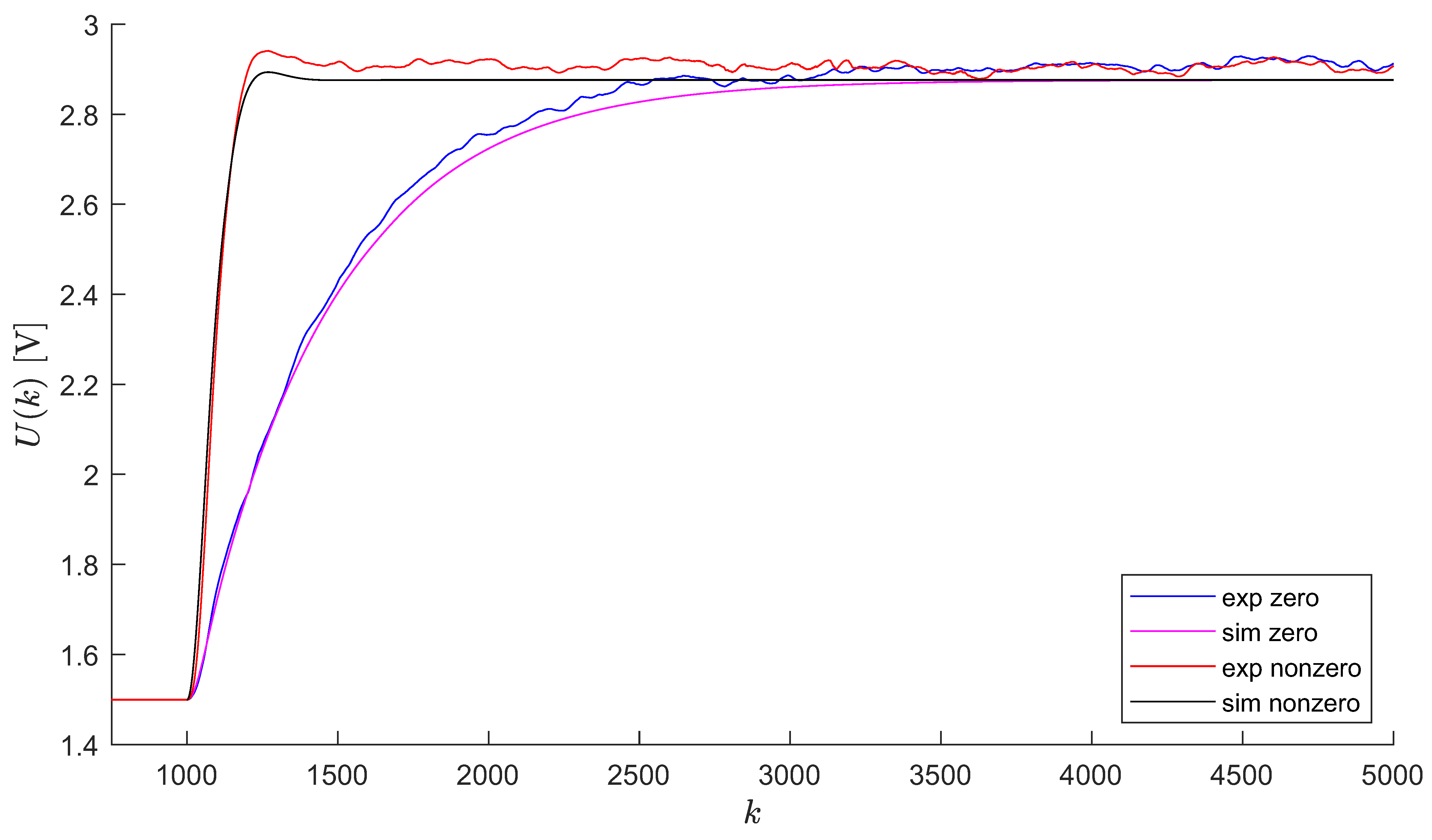
• Simulation and experimental results of comparing these two PDC controllers are presented to show that this paper’s technique is more comprehensive than the classical one because it considers nonzero initial conditions that the plant starts working from. The classical method offers parameters that should be universally optimal for any initial conditions, which is obviously not the case.

6. Conclusions

The research employed a new conditional optimization approach for linear discrete-time systems that is more suitable and appropriate than the traditional one. The optimization was performed in the parameter space of two unknown and variable parameters. The method is based on the works [43,45], which introduced the full transfer function matrix such that, in the study, the characteristic polynomial of the full transfer function matrix was employed during system conditional optimization rather than the classical transfer function. It was, more specifically, the characteristic polynomial of the row nondegenerate full transfer function matrix. In addition, a new, compact calculus [43,45] was utilized, without which it is impossible to determine the full transfer function matrix.

A different type of performance index was applied that was totally consistent with the use of the full transfer function matrix. The performance index was expressed as the sum of squared errors derived from the most realistic case, with the external input and nonzero initial conditions acting simultaneously on the system.

The constructed three individual linear first order PS controllers were combined to work as a PDC controller. As a result, in the design of a fuzzy controller using the PDC approach, the efficacy of the created fuzzy controller was connected to the previously constructed system model with fuzzy structure. To “capture” the nonlinearity in the real plant, a system model with a fuzzy structure was built.

An experimental example was provided to demonstrate the distinction in system performance when designed in the traditional and presented new way. Simulation and real experiments were used to determine the discrepancies. When the system was created in the traditional manner and began with nonzero initial conditions, the response was significantly poorer than when the system was designed in the novel manner and began with nonzero initial conditions as well. The results show that the improvement achieved, compared to individual controllers that take into account nonzero initial conditions applied to one local linear plant model [1,2], was transferred to the case discussed in this article, which is the application of a PDC control system to a nonlinear TS fuzzy plant model [25].

It was demonstrated that the optimal controller parameters for a given system at all zero initial conditions are not optimal for its operation under nonzero initial conditions, and this is shown in the paper for a nonlinear TS fuzzy model controlled by a PDC controller composed of three local linear first-order PS controllers. Figure 6 illustrates this concluding statement. Future research will focus on optimizing the TS fuzzy model using modern metaheuristic methods.

References

1. Gruyitch, L.; Bučevac, Z.; Jovanović, R.; Zarić, V. Discrete-Time System Conditional Optimisation in the Parameter Space via the Full Transfer Function Matrix. Trans. Famena 2021, 45, 45–62. [Google Scholar] [CrossRef]
2. Zarić, V.; Bučevac, Z.; Jovanović, R. Discrete-Time System Conditional Optimization in the Parameter Space with Nonzero Initial Conditions. Tech. Gaz. 2021, 29, 200–207. [Google Scholar] [CrossRef]
3. Prabhat Dev, M.; Sidharth, J.; Kumar, H.; Tripathi, B.N.; Khan, S.A. Various Tuning and Optimization Techniques Employed in PID Controller: A Review. In Proceedings of the International Conference in Mechanical and Energy Technology; Springer: Singapore, 2020; pp. 797–805. [Google Scholar]
4. Zhmud, V.; Hardt, W.; Stukach, O.V.; Dimitrov, L.; Nosek, J. The Parameter Optimization of the PID and PIDD Controller for a Discrete Object. In Proceedings of the 2019 Dynamics of Systems, Mechanisms and Machines (Dynamics), Omsk, Russia, 5–7 November 2019; pp. 1–6. [Google Scholar] [CrossRef]
5. Li, B.; Guo, X.; Zeng, X.; Dian, S. An optimal pid tuning method for a single-link manipulator based on the control parametrization technique. Discret. Contin. Dyn. Syst.-S 2020, 13, 1813–1823. [Google Scholar] [CrossRef]
6. Kurokawa, R.; Sato, T.; Vilanova, R.; Konishi, Y. Discrete-Time First-Order Plus Dead-Time Model-Reference Trade-off PID Control Design. Appl. Sci. 2019, 9, 3220. [Google Scholar] [CrossRef] [Green Version]
7. Li, Y.; Sheng, A.; Wang, Y. Synthesis of PID-type controllers without parametric models: A graphical approach. Energy Convers. Manag. 2008, 49, 2392–2402. [Google Scholar] [CrossRef]
8. Gryazina, E.N.; Polyak, B.T. Stability regions in the parameter space: D-decomposition revisited. Automatica 2006, 42, 13–26. [Google Scholar] [CrossRef]
9. Gryazina, E.N.; Polyak, B.T. Geometry of the stability domain in the parameter space: D-decomposition technique. In Proceedings of the 44th IEEE Conference on Decision and Control, Seville, Spain, 15 December 2005; pp. 6510–6515. [Google Scholar] [CrossRef]
10. Kipnis, M.; Nigmatullin, R. D-decomposition method for stability checking for trinomial linear difference equation with two delays. Int. J. Pure Apllied Math. 2016, 111, 479–489. [Google Scholar] [CrossRef] [Green Version]
11. Gryazina, E.N.; Polyak, B.T.; Tremba, A.A. D-decomposition technique state-of-the-art. Autom. Remote Control 2008, 69, 1991–2026. [Google Scholar] [CrossRef]
12. Sands, T. Control of DC Motors to Guide Unmanned Underwater Vehicles. Appl. Sci. 2021, 11, 2144. [Google Scholar] [CrossRef]
13. Hoyos, F.E.; Candelo-Becerra, J.E.; Rincón, A. Zero Average Dynamic Controller for Speed Control of DC Motor. Appl. Sci. 2021, 11, 5608. [Google Scholar] [CrossRef]
14. Kim, J.; Jon, U.; Lee, H. State-Constrained Sub-Optimal Tracking Controller for Continuous-Time Linear Time-Invariant (CT-LTI) Systems and Its Application for DC Motor Servo Systems. Appl. Sci. 2020, 10, 5724. [Google Scholar] [CrossRef]
15. Hoyos, F.E.; Candelo-Becerra, J.E.; Hoyos Velasco, C.I. Application of Zero Average Dynamics and Fixed Point Induction Control Techniques to Control the Speed of a DC Motor with a Buck Converter. Appl. Sci. 2020, 10, 1807. [Google Scholar] [CrossRef] [Green Version]
16. Akar Mehmet, T.I. Motion controller design for the speed control of DC servo motor. Int. J. Appl. Math. Inform. 2013, 7, 131–137. [Google Scholar]
17. Sabir, M.M.; Khan, J.A. Optimal Design of PID Controller for the Speed Control of DC Motor by Using Metaheuristic Techniques. Adv. Artif. Neural Syst. 2014, 2014, 1–8. [Google Scholar] [CrossRef] [Green Version]
18. Yordanova, S. Fuzzy logic approach to coupled level control. Syst. Sci. Control Eng. 2016, 4, 215–222. [Google Scholar] [CrossRef]
19. Chao, C.T.; Sutarna, N.; Chiou, J.S.; Wang, C.J. Equivalence between Fuzzy PID Controllers and Conventional PID Controllers. Appl. Sci. 2017, 7, 513. [Google Scholar] [CrossRef] [Green Version]
20. Tanaka, K.; Wang, H.O. Fuzzy Control Systems Design and Analysis; John Willey & Sons Inc.: New York, NY, USA, 2001. [Google Scholar] [CrossRef]
21. Vrkalovic, S.; Teban, T.A.; Borlea, L.D. Stable Takagi-Sugeno fuzzy control designed by optimization. Int. J. Artif. Intell. 2017, 15, 17–29. [Google Scholar]
22. Nguyen, A.T.; Taniguchi, T.; Eciolaza, L.; Campos, V.; Palhares, R.; Sugeno, M. Fuzzy Control Systems: Past, Present and Future. IEEE Comput. Intell. Mag. 2019, 14, 56–68. [Google Scholar] [CrossRef]
23. Xie, X.; Yue, D.; Zhang, H.; Xue, Y. Fault Estimation Observer Design for Discrete-Time Takagi–Sugeno Fuzzy Systems Based on Homogenous Polynomially Parameter-Dependent Lyapunov Functions. IEEE Trans. Cybern. 2017, 47, 2504–2513. [Google Scholar] [CrossRef]
24. Xie, X.; Yue, D.; Ma, T.; Zhu, X. Further Studies on Control Synthesis of Discrete-Time T-S Fuzzy Systems via Augmented Multi-Indexed Matrix Approach. IEEE Trans. Cybern. 2014, 44, 2784–2791. [Google Scholar] [CrossRef]
25. Jovanović, R.; Zarić, V. Identification and control of a heat flow system based on the Takagi-Sugeno fuzzy model using the grey wolf optimizer. Therm. Sci. 2022, 26, 2275–2286. [Google Scholar] [CrossRef]
26. Takagi, T.; Sugeno, M. Fuzzy identification of systems and its applications to modeling and control. IEEE Trans. Syst. Man Cybern. 1985, SMC-15, 116–132. [Google Scholar] [CrossRef]
27. Torres-Pinzón, C.A.; Paredes-Madrid, L.; Flores-Bahamonde, F.; Ramirez-Murillo, H. LMI-Fuzzy Control Design for Non-Minimum-Phase DC-DC Converters: An Application for Output Regulation. Appl. Sci. 2021, 11, 2286. [Google Scholar] [CrossRef]
28. Zhang, B.; Shin, Y.C. A Data-Driven Approach of Takagi-Sugeno Fuzzy Control of Unknown Nonlinear Systems. Appl. Sci. 2021, 11, 62. [Google Scholar] [CrossRef]
29. Chang, W.J.; Tsai, M.H.; Pen, C.L. Observer-Based Fuzzy Controller Design for Nonlinear Discrete-Time Singular Systems via Proportional Derivative Feedback Scheme. Appl. Sci. 2021, 11, 2833. [Google Scholar] [CrossRef]
30. Shasadeghi, M.; Safarinejadian, B.; Farughian, A. Parallel distributed compensator design of tank level control based on fuzzy Takagi-Sugeno model. Appl. Soft Comput. 2014, 21, 280–285. [Google Scholar] [CrossRef]
31. Seidi, M.; Markazi, A.H. Performance-oriented parallel distributed compensation. J. Frankl. Inst. 2011, 348, 1231–1244. [Google Scholar] [CrossRef]
32. Taniguchi, T.; Tanaka, K.; Yamafuji, K.; Wang, H. Nonlinear model following control via Takagi-Sugeno fuzzy model. In Proceedings of the 1999 American Control Conference (Cat. No. 99CH36251), San Diego, CA, USA, 2–4 June 1999; Volume 3, pp. 1837–1841. [Google Scholar] [CrossRef]
33. Viegas, D.; Batista, P.; Oliveira, P.; Silvestre, C. Distributed controller design and performance optimization for discrete-time linear systems. Optim. Control Appl. Methods 2021, 42, 126–143. [Google Scholar] [CrossRef]
34. Borrelli, F.; Baotić, M.; Bemporad, A.; Morari, M. Dynamic programming for constrained optimal control of discrete-time linear hybrid systems. Automatica 2005, 41, 1709–1721. [Google Scholar] [CrossRef]
35. Rosinová, D.; Hypiusová, M. Comparison of Nonlinear and Linear Controllers for Magnetic Levitation System. Appl. Sci. 2021, 11, 7795. [Google Scholar] [CrossRef]
36. Wang, Y.S.; Matni, N.; Doyle, J. Localized LQR optimal control. In Proceedings of the 53rd IEEE Conference on Decision and Control, Los Angeles, CA, USA, 15–17 December 2014. [Google Scholar] [CrossRef] [Green Version]
37. Hansson, A. A primal-dual interior-point method for robust optimal control of linear discrete-time systems. IEEE Trans. Autom. Control 2000, 45, 1639–1655. [Google Scholar] [CrossRef]
38. Orazbayev, B.B.; Ospanov, Y.A.; Orazbayeva, K.N.; Serimbetov, B.A. Multicriteria optimization in control of a chemical-technological system for production of benzene with fuzzy information. Bull. Tomsk Polytech. Univ. Geo Assets Eng. 2019, 330, 182–194. [Google Scholar] [CrossRef] [Green Version]
39. Orazbayev, B.; Zhumadillayeva, A.; Orazbayeva, K.; Iskakova, S.; Utenova, B.; Gazizov, F.; Ilyashenko, S.; Afanaseva, O. The System of Models and Optimization of Operating Modes of a Catalytic Reforming Unit Using Initial Fuzzy Information. Energies 2022, 15, 1573. [Google Scholar] [CrossRef]
40. Fel’dbaum, A.A. On the distribution of the roots of the characteristic equations of systems of regulation (in Russian). Avtom. I Telemeh. 1948, 9, 253–279. [Google Scholar]
41. Izmailov, R.N. The Peak Effect in Stationary Linear Systems with Scalar Inputs and Outputs. Autom. Remote Control 1987, 48, 1018–1024. [Google Scholar]
42. Polyak, B.; Tremba, A.; Khlebnikov, M.; Shcherbakov, P.; Smirnov, G. Large deviations in linear control systems with nonzero initial conditions. Autom. Remote Control 2015, 76, 957–976. [Google Scholar] [CrossRef]
43. Buchevats, Z.M.; Gruyitch, L.T. Linear Discrete-Time Systems; CRC Press/Taylor & Francis Group: Boca Raton, FL, USA, 2017. [Google Scholar]
44. Gruyitch, L. Advances in the Linear Dynamic Systems Theory; Llumina Press: Plantation, FL, USA, 2013. [Google Scholar]
45. Gruyitch, L. Linear Continuous-Time Systems; CRC Press: Boca Raton, FL, USA, 2017. [Google Scholar]
46. Sugeno, M.; Kang, G. Fuzzy modelling and control of multilayer incinerator. Fuzzy Sets Syst. 1986, 18, 329–345. [Google Scholar] [CrossRef]
47. Wang, H.; Tanaka, K.; Griffin, M. Parallel distributed compensation of nonlinear systems by Takagi-Sugeno fuzzy model. In Proceedings of the 1995 IEEE International Conference on Fuzzy Systems, Yokohama, Japan, 20–24 March 1995; Volume 2, pp. 531–538. [Google Scholar] [CrossRef]
48. Tanaka, K.; Sugeno, M. Stability analysis and design of fuzzy control systems. Fuzzy Sets Syst. 1992, 45, 135–156. [Google Scholar] [CrossRef]
49. Siljak, D.D. Analysis and Synthesis of Feedback Control Systems in the Parameter Plane I-Linear Continuous Systems. IEEE Trans. Appl. Ind. 1964, 83, 449–458. [Google Scholar] [CrossRef]
50. Siljak, D.D. Analysis and Synthesis of Feedback Control Systems in the Parameter Plane II-Sampled-Data Systems. IEEE Trans. Appl. Ind. 1964, 83, 458–466. [Google Scholar] [CrossRef]
51. Grujić, L.T. Discrete Systems (In Serbian); Faculty of Mechanical Engineering: Belgrade, Serbian, 1991. [Google Scholar]
52. Poularikas, A. Transforms and Applications Handbook; Electrical Engineering Handbook; CRC Press: Boca Raton, FL, USA, 2018. [Google Scholar]
Figure 1. Membership functions.
Applsci 12 07705 g001
Figure 2. The loci in the α β parameter plane of the constant damping coefficient ζ = 0.7 .
Applsci 12 07705 g002
Figure 3. Full block diagram of the closed loop system.
Applsci 12 07705 g003
Figure 4. Equivalent full block diagram of the closed loop system.
Applsci 12 07705 g004
Figure 5. The constant damping coefficient curve with optimal values applied to it for nonzero and zero initial conditions.
Applsci 12 07705 g005
Figure 6. Simulation and experimental results of designed PDC controllers that take into account zero and nonzero initial conditions.
Applsci 12 07705 g006
Figure 7. Simulation and experimental control signals of designed PDC controllers that take into account zero and nonzero initial conditions.
Applsci 12 07705 g007