Abstract
For comprehending the effect of tidal action on nitrogen cycle in silty-clay riparian hyporheic zones, the synchronous monitoring of water level and water quality was carried out along a test transect during a spring tidal period from 21 to 23 October 2021. Moreover, the permeability and chemical composition of soil samples from drilled holes were measured. Subsequently, the spatiotemporal variation of inorganic nitrogen concentrations in the groundwater in the riparian hyporheic zone was investigated during the study period, and the potential reason was discussed. It is shown that the delayed response time of groundwater level in the silty-clay riparian zone to the tide-driven fluctuation of the river stage increased with distance from the shore and reached 3.0 h at the position 3.83 m away from the shore. The continuous infiltration of the river water under tide action contributed to the aerobic and neutral riparian hyporheic zone conductive to nitrification. Within 4 m away from the bank, the dominant inorganic nitrogen form changed from -N to -N, upon increasing the distance from the bank. Additionally, the removal of nitrogen could occur in the riparian hyporheic zone with aerobic and neutral environment under the conjoint control of nitrification, microbial assimilation, and aerobic denitrification.
1. Introduction
In order to ensure the security of the global food supply, a large amount of nitrogen fertilizer has been utilized in the past few decades. For example, the average nitrogen utilization has achieved the rate of 305 kg/hm2 in China [1]. Excessive bioavailable nitrogen such as nitrate nitrogen () and ammonia nitrogen () in rivers will lead to water eutrophication and, consequently, damage the ecological balance of river systems. Particularly in coastal areas, nitrogen pollution in rivers is generally serious due to dense population and active industry and agriculture production. If it cannot be maintained under effective control, the excessive nitrogen will continue to enter the ocean and further affect the health of the coastal ecosystem and the sustainable utilization of marine resources.
Hyporheic zones of river ecosystem are water-saturated sediment (known as aquifer) below the riverbed and extending to the riparian areas on both sides. It is not only a key area for water exchange and solute migration between river and groundwater, but also an important place for microbial growth and metabolism. Mass exchange and energy transfer are frequent and biogeochemical reactions are complex within a hyporheic zone, which is of great significance to the structure, function, and health of river ecosystem [2,3,4]. Nitrogen is transported between rivers and their riparian zones through hyporheic exchange and transformed between different chemical forms (e.g., , , nitrite nitrogen (), and ) through biogeochemical reactions [5]. Therefore, to realize the effective control of nitrogen pollution in rivers, it is necessary to fully comprehend nitrogen migration and transformation in groundwater in hyporheic zones.
Nitrogen in groundwater in a hyporheic zone varies geographically, and its form changes temporally, which forms a complex dynamic cycle [6,7,8,9]. Some hydrological events (e.g., rainstorm, flooding, reservoir discharge, and tidal action) can change the recharge relationship between river water and groundwater, consequently influencing nitrogen migration in hyporheic zones [10,11,12,13]. Shibata et al. carried out onsite monitoring to study the water exchange and the change in nitrogen concentration in the hyporheic zone during the rainstorm. It was found that the increase in nitrogen concentration in the hyporheic zone was mainly caused by the rainwater infiltration through the overlying unsaturated zone rather than the lateral seepage from the river [14]. The research conducted by Singh et al. indicated that the flood process extended the mixing range of surface water and groundwater and had a significant impact on the mass cycle in the riverbed hyporheic zone [15]. Sawyer et al. studied the impact of the reservoir operation on the lateral hyporheic exchange, and the results showed that the impact range could extend to 1–5 m away from the shore [16]. Unlike the hydrological events mentioned above, tides exhibit periodicity, and the tidal period is usually about 12 or 24 h. This makes the hyporheic exchange more frequent and the biogeochemical process in the hyporheic zone more complex [17]. In recent years, there has been growing concern over the hyporheic zones of tidal rivers. Musial et al. quantified the tide-driven hyporheic exchange fluxes across the bank and the bed and deduced that the tidal bank storage in the sandy hyporheic zone might remove nutrients from rivers [18]. The geochemical measurements and numerical simulation performed by Barnes et al. showed that it was possible that the hyporheic zone with permeable sediment and low organic matter content could be a source of nitrate to the tidal river [19].
Hydrogeological conditions and ecological factors could affect the nitrogen cycle in hyporheic zones [20,21,22]. McGarr et al. investigated the hyporheic exchange process in a sand–gravel mixed riverbed and pointed it out that the pore water flowed preferentially through the sediment of high-permeability, which affected nitrogen transport pathways [23]. The sediment heterogeneity could result in the existence of tiny anoxic blocks within the aerobic zone near the shore, thus affecting nitrogen processing [24]. The retention time of river water is usually extended in the low-permeability riverbed sediment, which is beneficial to the full reaction between nitrogen and dissolved oxygen (DO) [25]. In addition, the migration ability of in the hyporheic zone may be limited to a certain extent due to the electrostatic attraction by soil particles [26]. Eco-environmental factors mainly include the reactant concentration, redox potential (Eh), temperature (T), and pH [27,28,29]. The nitrogen-related biogeochemical reactions such as nitrification and denitrification are greatly governed by DO concentration and Eh in hyporheic zones [30]. Dissolved organic carbon (DOC) is another key factor controlling the nitrogen cycle, and increasing DOC concentration could promote denitrification [31]. Zarnetske et al. found that DOC and DO could be preferentially consumed in the near-shore hyporheic zone [32]. Additionally, temperature could affect the microbial activity, reaction rate, and DO concentration, consequently influencing the process of nitrogen cycle in the hyporheic zone [33,34]. Some studies demonstrated that pH showed a positive correlation with concentration and a negative one with concentration [35].
Although the nitrogen cycle in hyporheic zones has been extensively studied, there is little work aiming at the case of low-permeability riparian hyporheic zones of tidal rivers. At present, the mechanism underlying how tides drive nitrogen migration and transformation in riparian hyporheic zones with low permeability sediment is not very clear. The main objective of the study was to characterize the spatiotemporal variations of various inorganic nitrogen concentrations in groundwater in poorly permeable hyporheic zones of tidal rivers and discuss the potential reason why such variations existed. A representative transect was chosen to carry out the drilling, monitoring, and sampling. By means of onsite monitoring and lab analysis, the response of the riparian groundwater level to the tide-driven fluctuation of the river stage was studied, the spatiotemporal variations of inorganic nitrogen concentrations in the groundwater in the riparian hyporheic zone were analyzed, and the potential influencing factors were discussed. The results are expected to enrich the theory of river hyporheic zones and provide a scientific basis for nitrogen pollution treatment of tidal rivers.
2. Methodology
2.1. Field Monitoring
The test site was located on the riverbank of the Jingzi River, a tributary of the Huangpu River in Shanghai, China, as illustrated in Figure 1. The Huangpu River, with a total length of approximately 114 km, is the last tributary of the Yangtze River before it empties into the East China Sea. The Huangpu River estuary forms a medium-tidal shallow-water environment where the tides are of irregular semidiurnal features. The tides can penetrate up to the Dianshan Lake and the provincial boundary between Zhejiang and Shanghai. On an average, the tidal period is about 12.5 h, where 4.5 h involves flooding and the remainder involves ebbing [36]. At the Wusong tide gauge station, the average tidal prism is about 5.8 × 10⁷ m3, the flood current velocity is up to 1.2 × 10⁴ m3/s, and the mean tidal range is about 2.27 m [37]. The test site was located about 29 km upstream of the Wusong tide gauge station. According to the preliminary research, there was a good response relationship between the river stages at the test site and the sea levels at Wusong station. The flooding at the test site was about 2.5 h behind that at Wusong station. Furthermore, the fluctuation range of the river stage at the site was up to approximately 0.5 m.
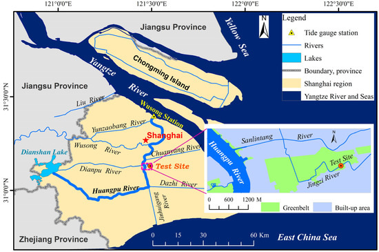
Figure 1.
Location of the test site.
The land use is mainly green field and residential in the surrounding area of the test site. The green field is unused and covered with bushes and stunted trees. The Jingzi River flows through the greenbelt, serving as a sewage channel of the vicinity. The terrain around the test site is relatively flat, and the slope degree of the bank is less than 9°. The riverbed sediment and the shallow aquifer materials at the site consist of silty-clay soils extensively distributed on the floodplain of the Huangpu River. The site with gentle slope, poorly permeable sediment, and less interference was considered suitable for the investigation.
The site was instrumented with a perpendicular transect of observation wells and sampling points, as shown in Figure 2. One observation well marked as WR0 was set in the river channel, and four other wells (i.e., WB1, WB2, WB3, and WB4) were laid on the riverbank, 0.71 m, 1.11 m, 2.43 m, and 3.85 m away from the shore, respectively (Figure 2a). The well pipes, made of polyvinyl chloride (PVC) material, were equipped with pipe covers at both ends. A hole punch was employed to make scattered tiny holes with a diameter of about 5 mm in the wall of the pipes. A nylon cloth with a mesh size of 0.15–0.20 mm was wrapped around each pipe. The wells on the riverbank were 200 cm in length and 11 cm in diameter, while WR0 was 80 cm in length and 6 cm in diameter. Each well tube was inserted vertically into the sediment. A high-precision GPS (Z-Survey i70, Manufacturer: CHCNAV Co. Ltd., Shanghai, China) and a leveling instrument (B30, Manufacturer: SOKKIA Co. Ltd., Tokyo, Japan) were used to survey the top elevation of each well. One water-level sensor (HOBO Kit-D-U20-04, Manufacturer: ONSET Co. Ltd., Bourne, Cape Cod, Centerville, MA, USA) was installed at the bottom of each well, with a data collection interval of 5 min.
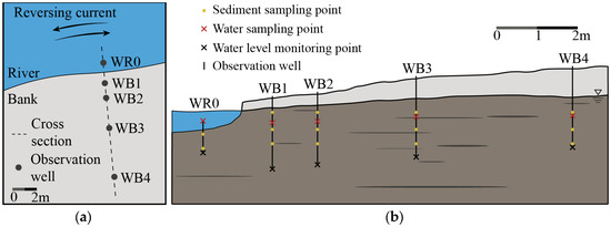
Figure 2.
The transect for monitoring and sampling: (a) the top view; (b) the cross-section.
According to the preliminary work, the fluctuation range of the Jingzi River stage was mostly less than 0.5 m, and the change in groundwater table could not be observed as the river stage fluctuation was smaller than 10 cm (usually occurred during neap tides). Thus, a spring tide period without rain should be chosen to focus on the impact of tides. According to the tide prediction table and the weather forecast information released in Shanghai, the 3 day spring tide period from 21 to 23 October 2021 was selected to carry out the monitoring of water level and water quality. The data recorded by the water-level sensors were exported and processed through atmospheric pressure correction. A portable dissolved oxygen meter (LDO™, Manufacturer: HACH Co. Ltd., Loveland, CO, USA) and a portable multiparameter water quality analyzer (sensION+ MM156, Manufacturer: HACH Co. Ltd., Loveland, CO, USA) were employed to synchronously determine DO concentration, temperature, and pH in the river channel and the four riparian wells.
2.2. Sample Collection
During the drilling of five wells, 14 columnar sediment samples with a diameter of 70 mm and height of 200 mm were collected using a stainless-steel soil sampler. The riverbed sediment samples were collected at the depths of 10–30 cm and 40–60 cm below the riverbed at WR0. Considering the depth distribution of the groundwater table in the riparian zone, the riparian sediment samples were individually collected at the depth of 40–120 cm below the surface at WB1, at the depth of 50–130 cm below the surface at WB2, at the depth of 100–180 cm below the surface at WB3, and at the depth of 120–200 cm below the surface at WB4. The three sediment samples were collected from each riparian borehole at equal intervals. All sediment samples were stored in the separate bags in a cooling box keeping the temperature below 5 °C and then taken back to the lab for testing within 24 h. Sediment samples collected were divided into two aliquots: one for determining the contents of total nitrogen (TN) and total carbon (TC), and the other for analyzing permeability coefficient (K), particle size, and sediment type.
Water samples were collected from the river and the four wells using a liquid sampling tube with a total capacity of 500 mL. Water sampling was carried out at 2 h intervals from 6:00 a.m. to 6:00 p.m. on any particular day of 21–23 October 2021. The water sampling points were 50 cm below the free water table. Figure 2b presents the positions of the sediment and water sampling points. The tube was cleaned with deionized water before sampling to avoid cross-contamination between water samples [38]. Water discharged from the tube was stored in both polyethylene vials of 200 mL and amber glass vials of 20 mL. The former vials were used for the concentration analysis of inorganic nitrogen (, , and ), while the latter vials were used for the DOC determination. All water samples were stored in the cooling box and subsequently taken back to the lab for testing within 24 h. Each water sample was filtered through a 0.45 μm filter membrane before testing.
2.3. Sample Analysis
TN content in each sediment sample was determined using a continuous flow analyzer (QuAAtro 39, Manufacturer: SEAL Co. Ltd., Norderstedt, Germany), while TC content was determined using a total organic carbon analyzer (TOC-VCPN, Manufacturer: Shimadzu Co. Ltd., Kyoto, Japan). Particle size was analyzed using a laser particle size meter (Mastersizer 3000, Manufacturer: Malvern Instrument Co. Ltd., Malvern, UK) with the measurement range of 0.01–3500 μm, after larger grains were removed through sieving. On the basis of the data from particle size analysis, the sediment type was determined. The sediment density (ρ) was quantified by the cutting ring method, and the permeability coefficient (K) was determined through the consolidation test.
For any water sample, concentration was determined using a continuous flow analyzer (QuAAtro 39, Manufacturer: SEAL Co. Ltd., Norderstedt, Germany) with a quantification limit of 0.02 mg/L, concentration was determined using an ion chromatograph (ICS-90, Manufacturer: DIONEX Co. Ltd., Sunnyvale, CA, USA) with a quantification limit of 0.02 mg/L, concentration was determined using a spectrophotometer (U-3010, Manufacturer: HITACHI Co. Ltd., Tokyo, Japan) with a quantification limit of 0.002 mg/L, and DOC concentration was determined using a total organic carbon analyzer (TOC-VCPN, Manufacturer: Shimadzu Co. Ltd., Kyoto, Japan).
2.4. Determination of Periodicityand Response Time of Water-Level Fluctuation
2.4.1. Periodicity
The frequency analysis of the river stage and the riparian groundwater level was carried out using the fast Fourier transform algorithm (FFT) in MATLAB. FFT is applied to transform signals from time domain to frequency domain for quickly analyzing the frequency characteristics of stationary or nonstationary signals. FFT is an optimization algorithm of discrete Fourier transform (DFT). The DFT can be defined as follows [39]:
where is the value in the n-th place of a sampled timeseries, is the length of the series, is the rotation factor equal to , and is the imaginary unit, .
Through the DFT mentioned above, spectrum values can be calculated, and the spectrum sequence can be obtained. In order to optimize the calculation efficiency, a sampled timeseries with the length of N is usually divided into two subsequences with the length of N/2 according to the symmetry and periodicity of . As a result, a pair of DFT units can reduce the computation amount from to , which is the reason why FFT is performed quickly. After the FFT calculation, the spectrum diagram can be plotted with signal frequency as the horizontal axis and amplitude as the vertical axis. The dominant oscillation frequency of the river stage or the groundwater level corresponded to the maximum spectrum value in the diagram; accordingly, the dominant period could be determined.
2.4.2. Delayed Response Time and Correlation
The response of the groundwater level to the rise and fall of the river stage was analyzed using the cross-correlation analysis method. Through cross-correlation analysis, the response relationship between the two timeseries could be estimated, and the time shift could be quantified. For two discrete timeseries signals and , their cross-correlation function is expressed in Equation (2) [40].
where m is the moment, M is the length of the timeseries, is the delayed time, and and are the timeseries of the river water level and the groundwater level, respectively. A larger value indicates a greater correlation between the two sequences. If is equal to , then represents the self-correlation function value of the two sequences at . Normalization is usually performed on , so that the self-correlation is equal to one at the delayed time of zero. The delayed response time of groundwater level to the rise and fall of the river stage corresponded to the maximum .
2.5. Statistical Analysis of Water Quality Parameters Data
The seven water quality parameters (, , , DO, DOC, pH, and temperature) were analyzed using analysis of variance (ANOVA) test and Welch’s test. Levene’s test was employed initially to determine whether the data met the hypothesis of homogeneity of variance. If the result rejected the hypothesis, Welch’s test was chosen to analyze the significance of differences in various water quality parameters of the groundwater among different riparian observation wells. Otherwise, the ANOVA test was used. The level of significance was set to p < 0.05 for both Welch’s test and the ANOVA test.
3. Results
3.1. Variation and Hysteresis of Groundwater Table in the Riparian Hyporheic Zone under Tidal Effect
The river stage fluctuated twice a day and was of irregular semidiurnal characteristics (Figure 3). During the monitoring period, the mean tidal duration was about 12.2 h. The maximum level was 1.196 m a.s.l., and the minimum level was 0.850 m a.s.l., which contributed to a fluctuation range of 34.6 cm.
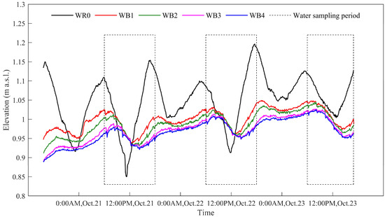
Figure 3.
Fluctuation curve of water level in the river channel (WR0) and the four riparian observation wells (WB1–WB4) during the monitoring period from 21 to 23 October 2021.
The groundwater level in any riparian well fluctuated twice a day, just like the river water stage (Figure 3). Regardless of the river channel or the riparian wells, the dominant oscillation period of the water level time series was 12.2 h. The fluctuation range of the water level gradually decreased upon increasing the distance from the shore on any monitoring day, as shown in Table 1. Over the 3 day study period, the fluctuation range of the daily mean river stage declined from 22.7 to 12.9 cm, while that of the daily mean groundwater level in each riparian well changed a little. Furthermore, the groundwater level in the riparian hyporheic zone exhibited a slow response to the rise and fall movement of the river stage. The delayed response time extended from 90 to 180 min, and the correlation coefficient decreased from 0.75 to 0.52, when the distance increased from 0.71 to 3.85 m away from the shore.

Table 1.
Fluctuations and the response relationship of the river stage and the groundwater level during the monitoring period from 21 to 23 October 2021.
During most of the monitoring period, the river stage was higher than the groundwater level and, hence, the river water continued to penetrate into the riparian hyporheic zone under such a hydraulic gradient. As a result, the groundwater level showed an overall upward trend (Figure 3). The daily mean groundwater levels in different riparian wells showed upward trends with the increase of 3.1–3.9 cm over the monitoring period (Figure 4a). Since the temperature of the river water was lower than that of the groundwater during the study period, the infiltration of the river water to the groundwater contributed to the drop in groundwater temperature. Although the river water temperature increased, the groundwater temperature in the riparian hyporheic zone declined (Figure 4b). Moreover, the decline range had a negative correlation with the distance from the shore. In view of the variations in water level and temperature of the groundwater at WB4, the migration range of water moisture and heat in the riparian hyporheic zone could reach 4 m away from the shore during the study period.
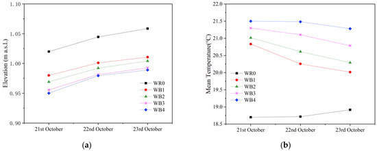
Figure 4.
Variations in (a) daily mean water level and (b) daily mean temperature of the river water and the groundwater over the monitoring period from 21 to 23 October 2021.
3.2. Spatial Distribution of Inorganic Nitrogen in the Riparian Hyporheic Zone
According to the statistical analysis, the concentration of three species of inorganic nitrogen (, , and ) in the groundwater showed significant differences among different riparian wells (p < 0.001). The mean concentration was 0.540 mg/L in the river channel, while those in the riparian observation wells ranged from 0.085 to 0.247 mg/L. This indicated that the concentration in the river water was higher than that in the riparian groundwater (Figure 5a). The mean concentrations in the groundwater in WB1, WB2, WB3, and WB4 were 0.085, 0.099, 0.247, and 0.105 mg/L, respectively. It is, thus, clear that the concentration in the groundwater in the riparian hyporheic zone was lower in the near-shore zone where WB1 and WB2 existed than in the offshore zone where WB3 and WB4 existed.
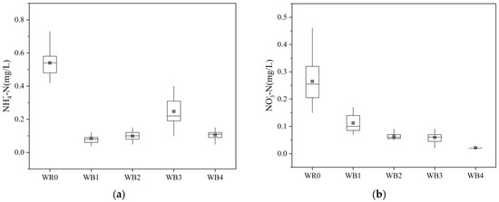
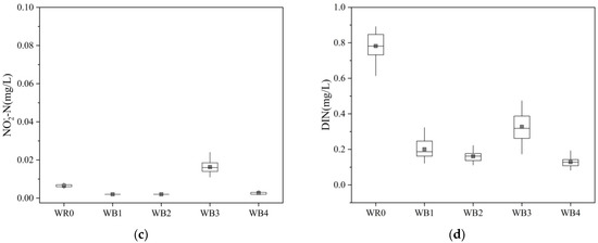
Figure 5.
Boxplots of the observed concentrations of inorganic nitrogen in the river water and the riparian groundwater during the study period from 21 to 23 October 2021: (a) ammonia nitrogen, ; (b) nitrate nitrogen, ; (c) nitrite nitrogen, ; (d) dissolved inorganic nitrogen, DIN.
The mean concentration was 0.265 mg/L in the river water and varied from 0.022 to 0.112 mg/L in the groundwater in the riparian wells (Figure 5b). This implies that the concentration in the river water was higher than that in the groundwater in the riparian hyporheic zone. The mean concentrations in the groundwater were 0.112, 0.062, 0.060, and 0.022 mg/L in WB1, WB2, WB3, and WB4, respectively. The mean concentrations in the riparian groundwater decreased gradually with increasing distance from the shore. The mean concentrations in both the river water and the groundwater in the four wells were below 0.02 mg/L (Figure 5c). This was mainly due to its chemical instability.
Dissolved inorganic nitrogen (DIN) was approximate to the sum of the concentrations of , , and . The mean DIN concentration was 0.782 mg/L in the river water and varied from 0.129 to 0.327 mg/L in the groundwater in the riparian wells (Figure 5d). The DIN concentration in the river water was higher than that in the riparian groundwater, and the offshore groundwater had a higher DIN concentration than the near-shore groundwater.
The content of in the groundwater accounted for about 56% of the total DIN content at WB1 on average and decreased with increasing distance from the shore (Figure 6). In contrast, the mean proportion gradually increased from 43% at WB1 to 81% at WB4. For any riparian well, the mean proportion kept the low value less than 5%.
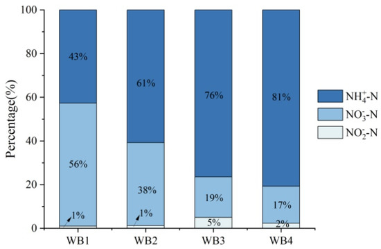
Figure 6.
Mean proportions of different forms of inorganic nitrogen in the groundwater in the riparian observation wells during the study period from 21 to 23 October 2021.
3.3. Temporal Variation of Inorganic Nitrogen Concentrations in the Riparian Hyporheic Zone
Over the study period, the daily mean concentration in the groundwater increased from 0.070 to 0.106 mg/L at WB1 and rose from 0.087 to 0.114 mg/L at WB2 (Figure 7a). In contrast, it decreased from 0.337 to 0.193 mg/L at WB3 and fell from 0.110 to 0.097 mg/L at WB4. It is distinctly clear that the daily mean concentration showed an upward trend in the near-shore zone and a downward one in the offshore zone.
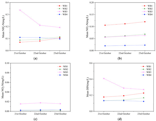
Figure 7.
Variations in daily mean inorganic nitrogen concentrations in the river water and the riparian groundwater over the study period from 21 to 23 October 2021: (a) ammonia nitrogen, ; (b) nitrate nitrogen, ; (c) nitrite nitrogen, ; (d) dissolved inorganic nitrogen, DIN.
Meanwhile, the daily mean concentration in the groundwater increased from 0.106 to 0.120 mg/L at WB1 and rose from 0.057 to 0.068 mg/L at WB2 (Figure 7b). However, it changed little in the offshore groundwater. The daily mean concentration in the riparian groundwater showed little change (Figure 7c). This is mainly due to the concentration having a very low concentration in both the river water and the riparian groundwater.
The daily mean DIN concentration increased from 0.178 to 0.228 mg/L at WB1 and ascended from 0.146 to 0.185 mg/L at WB2 (Figure 7d). It decreased from 0.408 to 0.271 mg/L at WB3 and fell from 0.132 to 0.123 mg/L at WB4. It is clear that the variation of the DIN concentration was roughly the same as that of the concentration in the groundwater; hence, was generally the dominant form of inorganic nitrogen in the riparian hyporheic zone within 4 m from the shore.
3.4. Physicochemical Characteristics of Sediment and Water in the River Channel and the Riparian Hyporheic Zone
There was a great difference between the horizontal and vertical permeability coefficients of the sediment in the riparian hyporheic zone (Table 2). For the sediment at any specific position, the horizontal permeability coefficient was 10 times higher than the vertical one, which implied that the lateral migrations of both the hyporheic flow and the solutes were dominant along the transect. According to the grain size distribution, the riparian sediment was determined as silty-clay soil.
Table 2.
Physical properties of the sediment in the riparian hyporheic zone.
Both the TN and the TC contents of the sediments gradually increased with depth, and the low contents of TN and TC appeared within the extent (0.9–1.05 m a.s.l.) where the riparian groundwater fluctuated (Figure 8). This could provide a clue that the extent where the groundwater level varied might be the hotspot of biogeochemical reactions in the riparian hyporheic zone, since large amounts of organic mass such as organic nitrogen and organic carbon were consumed in the course of the reactions involving micro-organisms. Furthermore, the mean TN content of the sediment at WB3 was the highest at 674 mg/kg, compared with that at the three other riparian wells.
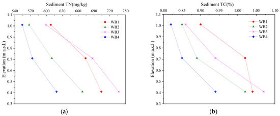
Figure 8.
Vertical distribution of the nitrogen and carbon contents of the riparian sediments: (a) total nitrogen, TN; (b) total carbon, TC.
The DO concentration in the groundwater showed a significant difference among different riparian wells (p < 0.05). The mean DO concentration in the river water was 6.24 mg/L, higher than that in the riparian groundwater (Figure 9a). Moreover, the mean DO concentration in the riparian groundwater decreased gradually with an increase in distance from the shore. The DO concentration of the riparian groundwater ranged from 5.2 to 6.8 mg/L. The difference of the DOC concentration in the groundwater was not significant among the riparian wells (p > 0.05). The data distribution range of the DOC concentration in the river water was less than that in the riparian groundwater (Figure 9b). This implies that the river water was not the only source of the DOC in the riparian groundwater.
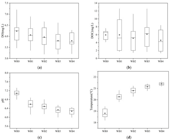
Figure 9.
Spatial variations of eco-environmental factors along the transect: (a) dissolved oxygen, DO; (b) dissolved organic carbon, DOC; (c) pH; (d) temperature.
There were significant differences in both the pH and the temperature in the groundwater among different riparian wells (p < 0.001). The mean pH of the river water was about 7.08 (Figure 9c), higher than that of the groundwater in any riparian well (ranging from 6.27 to 6.59). Along the transect, the pH decreased with increasing the distance from the shore. The mean temperature of the river water was 18.8 °C, while that of the groundwater in the riparian wells, ranging from 20.3 to 21.4 °C, increased gradually with an increase in distance from the shore (Figure 9d).
4. Discussion
During the study period, the pH and the DO concentrations in the groundwater in the four riparian wells varied from 6.27 to 6.59 (neutral environment) and from 5.2 to 6.8 mg/L, respectively. It is generally considered that an environment is aerobic if DO concentration is greater than 3 mg/L [41]. Thus, the riparian hyporheic zone within 4 m from the bank was an aerobic and neutral environment in favor of nitrification. In past studies, denitrification was regarded as an anaerobic process, and it was considered that denitrification would no longer occur if DO concentration was greater than 4.5 mg/L [42,43]. However, recent research results showed that denitrification could also occur in aerobic zones in soils due to the existence of aerobic denitrifying bacteria which could live in the environment with a DO concentration of 3–9 mg/L and a neutral pH [44,45,46]. It was, therefore, deduced that aerobic denitrification and nitrification might coexist in the riparian hyporheic zone studied, and the combination of these two effects was conducive to the removal of nitrogen from the riparian zone.
In the investigation, the concentration in the near-shore groundwater was lower than that in the offshore groundwater, and the lowest value found at WB1 closest to the bank. It was reported by Pan et al. that the concentration in the riparian groundwater decreased with increasing the distance from the bank of the nitrogen-rich river [47]. This is inconsistent with the results of our research. By comparison, it was found that there were significant differences in concentration in the river water and type of the sediment. The concentration in the river water was 0.9–1.5 mg/L, and the sediment mainly consisted of coarse sand in their research, while the former was 0.4–0.7 mg/L and the latter was silty-clay soil in our research. Some studies indicated that a low permeability of the sediment could reduce flow velocity of the pore water and, consequently, prolong the solute residence time, which provided the sufficient reaction time for nitrogen in the hyporheic zone [48,49]. Thus, the lower-permeability sediment and the river water with the lower nitrogen concentration contributed to more consumption and less recharge of the in the near-shore groundwater, respectively. This could explain why groundwater with less was observed in the near-shore hyporheic zone. However, upon increasing the distance from the bank, the DO concentration in the groundwater deceased gradually. The decline in DO concentration could lower the intensity of nitrification [50]. Furthermore, the mean TN content in the sediment at WB3 was highest among the four observation wells. The higher TN content could promote ammoniation, which is an important pathway for recharging the in the groundwater in hyporheic zones [51,52]. The greater recharge and lower consumption resulted in more existing in the groundwater in the offshore hyporheic zone.
The concentration in the riparian groundwater showed a downward trend as the distance from the bank increased along the test transect. This matches with the work of Zhang et al. [53]. Due to the strong nitrification reactions and the recharge from the river water, the was enriched in the near-shore groundwater. However, in the offshore hyporheic zone with the poorly permeable sediment, the recharge of from the river water was very slow and could take several hours or even more according to the delayed response time of the groundwater level to the river stage in the study. Moreover, due to the decline in DO concentration, a lower amount of the in the groundwater was produced by nitrification. Additionally, the riparian zone beyond 2 m away from the bank was covered with undisturbed shrubs. According to the research conducted by Stark and Hart, the microbial communities in the soil under undisturbed forest ecosystems had the capacity to assimilate most of the produced by nitrification [54]. Hence, the microbial assimilation of could be considered as a reason for the in the offshore groundwater being lower than that in the near-shore groundwater.
During most of the study period, the river stage remained higher than the riparian groundwater level under tide action, which led to a continuous infiltration of river water into the riverbank. As the river water steadily flowed into the hyporheic zone, the and in the near-shore groundwater were continuously recharged; thus, the and concentrations showed overall upward trends in the near-shore zone over the 3 day study period. Accompanied by the seepage process, the riparian groundwater level had an uplift which made part of the oxygen in the upper vadose zone enter the groundwater [55]. Thus, the DO concentration in the riparian groundwater increased due to the lateral recharge from the river, as well as the vertical recharge from the upper soil, which contributed to a whole aerobic environment within 4 m from the bank. The increase in DO concentration in the offshore groundwater promoted nitrification [56]. Meanwhile, the fine particles of the silty clay sediment had strong adsorption capacity, which restricted the further migration of the in the near-shore groundwater to some extent [57]. For these reasons, the concentration in the offshore groundwater decreased over the study period. Although the further migration of the in the near-shore groundwater and nitrification could have caused an increase in concentration in the offshore groundwater, little change was actually observed. This might be due to the fact that the microbial assimilation of was considerable in the offshore hyporheic zone under the shrubs.
The variation range of the DOC concentration in the groundwater in each riparian well was significantly larger than that in the river. The DOC in the riparian groundwater mainly depended on the dissolution of particulate organic carbon (POC) in the sediment rather than the infiltration of the river water, which is consistent with the research of Peyrard et al. [58]. Some previous studies reported the effect of DOC, pH, and temperature on the nitrogen cycle in the hyporheic zone. The DOC could play an important role in denitrification processes [59]. The reaction rate of nitrogen could be inhibited in an acidic environment (pH < 5.5), but there is an insignificant impact on nitrogen cycle in a neutral environment [60,61]. The nitrification rate in soils gradually increases with temperature within the range of 15–35 °C [62]. However, in our research, there was an insignificant difference in DOC concentration in the riparian groundwater. Moreover, the pH remained neutral, and the temperature had a small change of 1–2 °C in the riparian hyporheic zone. Hence, DOC concentration, pH, and temperature may not be the dominant factors causing the spatiotemporal difference in inorganic nitrogen concentration in the groundwater in the riparian zone studied.
Additionally, it should be noted that the time period involved in the research was a spring tidal period in October, and recharging the riparian aquifers from the river water was dominant during the period. However, the tide-driven hyporheic exchange process varies with tide strength and season. Since the hyporheic exchange greatly influences the nitrogen occurrence, the findings of the study have to be seen in light of some limitations. Future research will be performed to analyze nitrogen occurrence in groundwater in silty-clay hyporheic zones under the action of tides of different strength and its seasonal variation. Moreover, the variations of nitrogen forms and the influencing factors with depth will need to be investigated to reveal the vertical nitrogen cycle in hyporheic zones of tidal rivers.
5. Conclusions
It was confirmed from the study that the groundwater level in the silty-clay riparian zone presented a slow response to the tide-driven fluctuation of the river stage. The delayed response time reached a few hours within 1–4 m away from the bank, which could help to extend the hydraulic and solute retention time. The continuous infiltration of the river water under tide action contributed to the aerobic and neutral riparian hyporheic zone conductive to nitrification. Within 4 m away from the bank, the dominant inorganic nitrogen form changed from -N to -N, upon increasing the distance from the bank. In addition, the removal of nitrogen could occur in the riparian hyporheic zone with an aerobic and neutral environment under the joint control of nitrification, microbial assimilation, and aerobic denitrification. It is important to consider that nitrogen occurrence in riparian hyporheic zones of tidal rivers is governed by many factors including tidal strength, permeability and chemical compositions of sediments, DO concentration, vegetation coverage, and even nitrogen concentration in river water.
Author Contributions
Conceptualization, Y.C. and J.X.; methodology, Y.C. and J.X.; software, J.X.; validation, J.X.; formal analysis, Y.C. and J.X.; investigation, Y.C., J.X., N.Z., R.H., X.R. and D.Y.; resources, Y.C. and J.X.; data curation, J.X., R.H. and X.R.; writing—original draft preparation, Y.C. and J.X.; writing—review and editing, Y.C. and N.Z.; funding acquisition, Y.C. and N.Z. All authors have read and agreed to the published version of the manuscript.
Funding
This research was financially supported by the National Natural Science Foundation of China (Grant No. 42077176) and the Natural Science Foundation of Shanghai (Grant No. 20ZR1459700).
Institutional Review Board Statement
Not applicable.
Informed Consent Statement
Not applicable.
Data Availability Statement
Data are contained within the article.
Acknowledgments
The authors specially thank the Shanghai Institute of Geological Survey for providing assistance with sample testing.
Conflicts of Interest
The authors declare no conflict of interest.
References
- Wang, Y.C.; Lu, Y.L. Evaluating the potential health and economic effects of nitrogen fertilizer application in grain production systems of China. J. Clean. Prod. 2020, 264, 121635. [Google Scholar] [CrossRef]
- Liang, D.; Song, J.X.; Xia, J.; Chang, J.B.; Kong, F.H.; Sun, H.T.; Wu, Q.; Cheng, D.D.; Zhang, Y.X. Effects of heavy metals and hyporheic exchange on microbial community structure and functions in hyporheic zone. J. Environ. Manag. 2022, 303, 114201. [Google Scholar] [CrossRef] [PubMed]
- Ward, A.S. The evolution and state of interdisciplinary hyporheic research. Wiley Interdiscip. Wiley Interdiscip. Rev. Water 2016, 3, 83–103. [Google Scholar]
- Cai, Y.; Shi, T.; Yao, J.L.; Liu, S.G.; Ruan, X.K.; Xu, J. Advance in field monitoring research of hydrodynamic process of hyporheic exchange in rivers. Adv. Water Sci. 2021, 32, 638–648. (In Chinese) [Google Scholar]
- Bernal, S.; Lupon, A.; Ribot, M.; Sabater, F.; Marti, E. Riparian and in-stream controls on nutrient concentrations and fluxes in a headwater forested stream. Biogeosciences 2015, 12, 1941–1954. [Google Scholar] [CrossRef] [Green Version]
- Lamontagne, S.; Cosme, F.; Minard, A.; Holloway, A. Nitrogen attenuation, dilution and recycling in the intertidal hyporheic zone of a subtropical estuary. Hydrol. Earth Syst. Sci. 2018, 22, 4083–4096. [Google Scholar] [CrossRef] [Green Version]
- Hampton, T.B.; Zarnetske, J.P.; Briggs, M.A.; Singha, K.; Harvey, J.W.; Day-Lewis, F.D.; Dehkordy, F.M.; Lane, J.W. Residence time controls on the fate of nitrogen in flow-through lakebed sediments. J. Geophys. Res.-Biogeosci. 2019, 124, 689–707. [Google Scholar] [CrossRef]
- Naranjo, R.C.; Niswonger, R.G.; Davis, C.J. Mixing effects on nitrogen and oxygen concentrations and the relationship to mean residence time in a hyporheic zone of a riffle-pool sequence. Water Resour. Res. 2015, 51, 7202–7217. [Google Scholar] [CrossRef]
- Zhou, N.Q.; Zhao, S.; Shen, X.P. Nitrogen cycle in the hyporheic zone of natural wetlands. Chin. Sci. Bull. 2014, 59, 2945–2956. [Google Scholar] [CrossRef]
- Wen, H.; Perdrial, J.; Abbott, B.W.; Bernal, S.; Dupas, R.; Godsey, S.E.; Harpold, A.; Rizzo, D.; Underwood, K.; Adler, T.; et al. Temperature controls production but hydrology regulates export of dissolved organic carbon at the catchment scale. Hydrol. Earth Syst. Sci. 2020, 24, 945–966. [Google Scholar] [CrossRef] [Green Version]
- Ledesma, J.L.J.; Ruiz-Perez, G.; Lupon, A.; Poblador, S.; Futter, M.N.; Sabater, F.; Bernal, S. Future changes in the Dominant Source Layer of riparian lateral water fluxes in a subhumid Mediterranean catchment. J. Hydrol. 2021, 595, 126014. [Google Scholar] [CrossRef]
- Newcomer, M.E.; Hubbard, S.S.; Fleckenstein, J.H.; Maier, U.; Schmidt, C.; Thullner, M.; Ulrich, C.; Flipo, N.; Rubin, Y. Influence of hydrological perturbations and riverbed sediment characteristics on hyporheic zone respiration of CO2 and N2. J. Geophys. Res.-Biogeosci. 2018, 123, 902–922. [Google Scholar] [CrossRef] [Green Version]
- Cai, Y.; Xing, J.W.; Ruan, X.K.; Zhong, N.Q.; Huang, R.Y.; Yi, D.Z. Advances in the numerical simulation of the migration and transformation of nitrogen in hyporheic zones of rivers. Water Resour. Prot. 2022. Available online: http://kns.cnki.net/kcms/detail/32.1356.TV.20220419.1738.004.html (accessed on 20 April 2022). (In Chinese).
- Shibata, H.; Sugawara, O.; Toyoshima, H.; Wondzell, S.M.; Nakamura, F.; Kasahara, T.; Swanson, F.J.; Sasa, K. Nitrogen dynamics in the hyporheic zone of a forested stream during a small storm, Hokkaido, Japan. Biogeochemistry 2004, 69, 83–103. [Google Scholar] [CrossRef] [Green Version]
- Singh, T.; Wu, L.W.; Gomez-Velez, J.D.; Lewandowski, J.; Hannah, D.M.; Krause, S. Dynamic hyporheic zones: Exploring the role of peak flow events on bedform-induced hyporheic exchange. Water Resour. Res. 2019, 55, 218–235. [Google Scholar] [CrossRef]
- Sawyer, A.H.; Cardenas, M.B.; Bomar, A.; Mackey, M. Impact of dam operations on hyporheic exchange in the riparian zone of a regulated river. Hydrol. Process 2009, 23, 2129–2137. [Google Scholar] [CrossRef]
- Bernhardt, E.S.; Blaszczak, J.R.; Ficken, C.D.; Fork, M.L.; Kaiser, K.E.; Seybold, E.C. Control points in ecosystems: Moving beyond the hot Spot hot moment concept. Ecosystems 2017, 20, 665–682. [Google Scholar] [CrossRef]
- Musial, C.T.; Sawyer, A.H.; Barnes, R.T.; Bray, S.; Knights, D. Surface water-groundwater exchange dynamics in a tidal freshwater zone. Hydrol. Process 2016, 30, 739–750. [Google Scholar] [CrossRef]
- Barnes, R.T.; Sawyer, A.H.; Tight, D.M.; Wallace, C.D.; Hastings, M.G. Hydrogeologic controls of surface water-groundwater nitrogen dynamics within a tidal freshwater zone. J. Geophys. Res.-Biogeosci. 2019, 124, 3343–3355. [Google Scholar] [CrossRef] [Green Version]
- Wallace, C.D.; Sawyer, A.H.; Soltanian, M.R.; Barnes, R.T. Nitrate removal within heterogeneous riparian aquifers under tidal influence. Geophys. Res. Lett. 2020, 47, e2019GL085699. [Google Scholar] [CrossRef]
- Wallace, C.D.; Sawyer, A.H.; Barnes, R.T.; Soltanian, M.R.; Gabor, R.S.; Wilkins, M.J.; Moore, M.T. A model analysis of the tidal engine that drives nitrogen cycling in coastal riparian aquifers. Water Resour. Res. 2020, 56, e2019WR025662. [Google Scholar] [CrossRef]
- Pryshlak, T.T.; Sawyer, A.H.; Stonedahl, S.H.; Soltanian, M.R. Multiscale hyporheic exchange through strongly heterogeneous sediments. Water Resour. Res. 2015, 51, 9127–9140. [Google Scholar] [CrossRef] [Green Version]
- McGarr, J.T.; Wallace, C.D.; Ntarlagiannis, D.; Sturmer, D.M.; Soltanian, M.R. Geophysical mapping of hyporheic processes controlled by sedimentary architecture within compound bar deposits. Hydrol. Process 2021, 35, e14358. [Google Scholar] [CrossRef]
- Briggs, M.A.; Day-Lewis, F.D.; Zarnetske, J.P.; Harvey, J.W. A physical explanation for the development of redox microzones in hyporheic flow. Geophys. Res. Lett. 2015, 42, 4402–4410. [Google Scholar] [CrossRef]
- Krause, S.; Tecklenburg, C.; Munz, M.; Naden, E. Streambed nitrogen cycling beyond the hyporheic zone: Flow controls on horizontal patterns and depth distribution of nitrate and dissolved oxygen in the upwelling groundwater of a lowland river. J. Geophys. Res.-Biogeosci. 2013, 118, 54–67. [Google Scholar] [CrossRef]
- Zhao, L.; Li, Y.L.; Wang, S.D.; Wang, X.Y.; Meng, H.Q.; Luo, S.H. Adsorption and transformation of ammonium ion in a loose-pore geothermal reservoir: Batch and column experiments. J. Contam. Hydrol. 2016, 192, 50–59. [Google Scholar] [CrossRef] [PubMed]
- Shan, J.; Yang, P.P.; Shang, X.X.; Rahman, M.M.; Yan, X.Y. Anaerobic ammonium oxidation and denitrification in a paddy soil as affected by temperature, pH, organic carbon, and substrates. Biol. Fertil. Soils 2018, 54, 341–348. [Google Scholar] [CrossRef]
- Bai, B.; Jiang, S.C.; Liu, L.L.; Li, X.; Wu, H.Y. The transport of silica powders and lead ions under unsteady flow and variable injection concentrations. Powder Technol. 2021, 387, 22–30. [Google Scholar] [CrossRef]
- Helton, A.M.; Ardon, M.; Bernhardt, E.S. Thermodynamic constraints on the utility of ecological stoichiometry for explaining global biogeochemical patterns. Ecol. Lett. 2015, 18, 1049–1056. [Google Scholar] [CrossRef]
- Pescimoro, E.; Boano, F.; Sawyer, A.H.; Soltanian, M.R. Modeling influence of sediment heterogeneity on nutrient cycling in streambeds. Water Resour. Res. 2019, 55, 4082–4095. [Google Scholar] [CrossRef]
- Zarnetske, J.P.; Haggerty, R.; Wondzell, S.M.; Baker, M.A. Labile dissolved organic carbon supply limits hyporheic denitrification. J. Geophys. Res.-Biogeosci. 2011, 116, G04036. [Google Scholar] [CrossRef] [Green Version]
- Zarnetske, J.P.; Haggerty, R.; Wondzell, S.M.; Baker, M.A. Dynamics of nitrate production and removal as a function of residence time in the hyporheic zone. J. Geophys. Res.-Biogeosci. 2011, 116, G01025. [Google Scholar] [CrossRef] [Green Version]
- Herrman, K.S.; Bouchard, V.; Moore, R.H. Factors affecting denitrification in agricultural headwater streams in Northeast Ohio, USA. Hydrobiologia 2008, 598, 305–314. [Google Scholar] [CrossRef]
- Bai, B.; Nie, Q.K.; Zhang, Y.K.; Wang, X.L.; Hu, W. Cotransport of heavy metals and SiO2 particles at different temperatures by seepage. J. Hydrol. 2021, 597, 125771. [Google Scholar] [CrossRef]
- Zhao, S.; Zhou, N.Q.; Shen, X.P. Driving mechanisms of nitrogen transport and transformation in lacustrine wetlands. Sci. China-Earth Sci. 2016, 59, 464–476. [Google Scholar] [CrossRef]
- Zong, H.C.; Zhang, W.S.; Zhang, J.S. Study on influence of sea level rise on storm tidal levels of Huangpu River. Yangtze River 2014, 45, 1–3. (In Chinese) [Google Scholar]
- Huang, X.Y. Hydrological characteristics of Shanghai area. J. China Hydrol. 1987, 32, 43–46. (In Chinese) [Google Scholar]
- Harvey, J.W.; Bohlke, J.K.; Voytek, M.A.; Scott, D.; Tobias, C.R. Hyporheic zone denitrification: Controls on effective reaction depth and contribution to whole-stream mass balance. Water Resour. Res. 2013, 49, 6298–6316. [Google Scholar] [CrossRef]
- Marcotte, D. Fast variogram computation with FFT. Comput. Geosci. 1996, 22, 1175–1186. [Google Scholar] [CrossRef]
- Qian, W.M.; Liang, H.Y.; Yang, G.Q. Applied Stochastic Processes, 1st ed.; Higher Education Press: Beijing, China, 2014; pp. 101–109. (In Chinese) [Google Scholar]
- Anderson, T.H.; Taylor, G.T. Nutrient pulses, plankton blooms, and seasonal hypoxia in western Long Island Sound. Estuaries 2001, 24, 228–243. [Google Scholar] [CrossRef]
- Xue, D.M.; Botte, J.; De Baets, B.; Accoe, F.; Nestler, A.; Taylor, P.; Van Cleemput, O.; Berglund, M.; Boeckx, P. Present limitations and future prospects of stable isotope methods for nitrate source identification in surface- and groundwater. Water Res. 2009, 43, 1159–1170. [Google Scholar] [CrossRef]
- Patureau, D.; Bernet, N.; Delgenes, J.P.; Moletta, R. Effect of dissolved oxygen and carbon-nitrogen loads on denitrification by an aerobic consortium. Appl. Microbiol. Biotechnol. 2000, 54, 535–542. [Google Scholar] [CrossRef] [PubMed]
- Huang, T.L.; Zhou, S.L.; Zhang, H.H.; Bai, S.Y.; He, X.X.; Yang, X. Nitrogen removal characteristics of a newly isolated indigenous aerobic denitrifier from oligotrophic drinking water reservoir, Zoogloeasp N299. Int. J. Mol. Sci. 2015, 16, 10038–10060. [Google Scholar] [CrossRef] [PubMed] [Green Version]
- Kim, M.; Jeong, S.Y.; Yoon, S.J.; Cho, S.J.; Kim, Y.H.; Kim, M.J.; Ryu, E.Y.; Lee, S.J. Aerobic denitrification of pseudomonas putida AD-21 at different C/N ratios. J. Biosci. Bioeng. 2008, 106, 498–502. [Google Scholar] [CrossRef] [PubMed]
- Hu, J.A.; Yang, X.Y.; Deng, X.Y.; Liu, X.M.; Yu, J.X.; Chi, R.; Xiao, C.Q. Isolation and nitrogen removal efficiency of the heterotrophic nitrifying-aerobic denitrifying strain K17 from a rare earth element leaching site. Front. Microbiol. 2022, 13, 905409. [Google Scholar] [CrossRef]
- Pan, J.; Li, R.F.; Meng, X.T.; Ye, M.X. Biogeochemical characteristics of nitrogen migrogen and transformation in subsurface flow belt driven by river collection. Environ. Eng. 2021, 39, 62–68. (In Chinese) [Google Scholar]
- Yabusaki, S.B.; Wilkins, M.J.; Fang, Y.L.; Williams, K.H.; Arora, B.; Bargar, J.; Beller, H.R.; Bouskill, N.J.; Brodie, E.L.; Christensen, J.N.; et al. Water table dynamics and biogeochemical cycling in a shallow, variably-saturated floodplain. Environ. Sci. Technol. 2017, 51, 3307–3317. [Google Scholar] [CrossRef]
- Krause, S.; Blume, T.; Cassidy, N.J. Investigating patterns and controls of groundwater up-welling in a lowland river by combining Fibre-optic Distributed Temperature Sensing with observations of vertical hydraulic gradients. Hydrol. Earth Syst. Sci. 2012, 16, 1775–1792. [Google Scholar] [CrossRef] [Green Version]
- Zarnetske, J.P.; Haggerty, R.; Wondzell, S.M.; Bokil, V.A.; Gonzalez-Pinzon, R. Coupled transport and reaction kinetics control the nitrate source-sink function of hyporheic zones. Water Resour. Res. 2012, 48, W11508. [Google Scholar]
- Marumoto, T.; Anderson, J.P.E.; Domsch, K.H. Decomposition of 14C- and 15N-labelled microbial cells in soil. Soil Biol. Biochem. 1982, 14, 461–467. [Google Scholar] [CrossRef]
- Weatherill, J.J.; Krause, S.; Ullah, S.; Cassidy, N.J.; Levy, A.; Drijfhout, F.P.; Rivett, M.O. Revealing chlorinated ethene transformation hotspots in a nitrate-impacted hyporheic zone. Water Res. 2019, 161, 222–231. [Google Scholar] [CrossRef]
- Zhang, Y.; Yang, P.H.; Wang, J.L.; Xie, S.Y.; Chen, F.; Zhan, Z.J.; Ren, J.; Zhang, H.Y.; Liu, D.W.; Meng, Y.K. Geochemical characteristics of lateral hyporheic zone between the river water and groundwater, a case study of Maanxi in Chongqing. Environ. Sci. 2016, 37, 2478–2486. (In Chinese) [Google Scholar]
- Stark, J.M.; Hart, S.C. High rates of nitrification and nitrate turn-over in undisturbed coniferous forests. Nature 1997, 385, 61–64. [Google Scholar] [CrossRef]
- Williams, M.D.; Oostrom, M. Oxygenation of anoxic water in a fluctuating water table system: An experimental and numerical study. J. Hydrol. 2000, 230, 70–85. [Google Scholar] [CrossRef]
- Covatti, G.; Grischek, T. Sources and behavior of ammonium during riverbank filtration. Water Res. 2021, 191, 116788. [Google Scholar] [CrossRef]
- Wu, F.; Wang, Y.; Yan, X.; Xia, C.; Xiao, Y.; Huo, J.; Zhou, X. Adsorption characteristics of suspended sediment to ammonia nitrogen in Lanzhou section of the Yellow River. China J. Environ. Eng. 2014, 8, 3201–3207. [Google Scholar]
- Peyrard, D.; Delmotte, S.; Sauvage, S.; Namour, P.; Gerino, M.; Vervier, P.; Sanchez-Perez, J.M. Longitudinal transformation of nitrogen and carbon in the hyporheic zone of an N-rich stream: A combined modelling and field study. Phys. Chem. Earth 2011, 36, 599–611. [Google Scholar] [CrossRef] [Green Version]
- Bohlke, J.K.; Antweiler, R.C.; Harvey, J.W.; Laursen, A.E.; Smith, L.K.; Smith, R.L.; Voytek, M.A. Multi-scale measurements and modeling of denitrification in streams with varying flow and nitrate concentration in the upper Mississippi River basin, USA. Biogeochemistry 2009, 93, 117–141. [Google Scholar] [CrossRef] [Green Version]
- Lehtovirta-Morley, L.E.; Stoecker, K.; Vilcinskas, A.; Prosser, J.I.; Nicol, G.W. Cultivation of an obligate acidophilic ammonia oxidizer from a nitrifying acid soil. Proc. Natl. Acad. Sci. USA 2011, 108, 15892–15897. [Google Scholar] [CrossRef] [Green Version]
- Kemmitt, S.J.; Wright, D.; Goulding, K.W.T.; Jones, D.L. pH regulation of carbon and nitrogen dynamics in two agricultural soils. Soil Biol. Biochem. 2006, 38, 898–911. [Google Scholar] [CrossRef]
- Hu, R.; Wang, X.P.; Pan, Y.X.; Zhang, Y.F.; Zhang, H. The response mechanisms of soil N mineralization under biological soil crusts to temperature and moisture in temperate desert regions. Eur. J. Soil Biol. 2014, 62, 66–73. [Google Scholar] [CrossRef]
Publisher’s Note: MDPI stays neutral with regard to jurisdictional claims in published maps and institutional affiliations. |
© 2022 by the authors. Licensee MDPI, Basel, Switzerland. This article is an open access article distributed under the terms and conditions of the Creative Commons Attribution (CC BY) license (https://creativecommons.org/licenses/by/4.0/).