Mapping Robot Singularities through the Monte Carlo Method

Abstract

In addition to other things, a robot’s design also determines its singularity configurations and points in the workspace. In designing the robot’s working trajectory, one of the main issues of robot steering is avoiding singularities. The article proposes a different approach to calculating the inverse task, which lies in the random mapping of the robot mechanism’s workspace through searching for points closest in proximity to the trajectory in question. The new methodology of mapping and detecting the states of singularity in the workspace is actually based on Monte Carlo analysis, since we were also interested in the number of occurrences. In terms of mathematical analysis, this method is less demanding, because in searching for joint variables suitable for the given trajectory, it does not use inverse calculation. It is important that the method is chosen appropriately. The method is sufficiently illustrative in the form of a graph, making, e.g., programming optimization simpler. The ultimate effect is the reduced time needed for computing joint variables and the availability of an option to select a robot configuration suitable for carrying out the required work. The paper offers an example of an analysis concerning three different robots.

1. Introduction

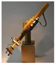
At the Department of Production systems and Robotics, Faculty of Mechanical Engineering, Technical University of Košice [1], we are developing our own concept of a robotic arm with a modular structure. The arm features variable DOF (degrees of freedom), but our priority is to fine-tune the practical 6 DOF. The kinematic arrangement of the robotic arm is serial, with multiangle curvatures between individual autonomous modules. The robot is referred to by its acronym of URM (unlimited rotation module). In contrast to common designs of serial kinematics in angular arrangement, the design of our modular robot features several specificities and peculiarities [2]. A few solutions similar to ours can even be found on the market. However, none of them contains as many innovations as the solution proposed by us. The advantages of the URM’s modular setup include the full autonomy of each module (in terms of its mechanics, data, power), wireless power transmission between individual modules (achieved through wireless power modules similar to those used in wireless charging of modern mobile phones), that the entire setup does not include a cable harness, and that therefore each module can rotate indefinitely, without any angular constraint. Passive curvatures between the individual modules may have various angular values, and thus have a direct effect on the size and shape of the robot’s workspace. Each module is energetically independently (each module contains powerful accumulators enabling the robot to function for a certain time when the feed from the mains is interrupted). Some of the main disadvantages of our modular design are the reduced load-bearing capacity of the robot’s end effector, reduced power efficiency compared to the standard cable harness arrangement, more complicated steering, and the occurrence of singular states. It was exactly the last of the items mentioned that necessitated further investigation and finding a solution.

It goes without saying that one of the main goals is to maximally reduce the costs of maintenance of such a modular system, which is in line with the solutions promoted under I4.0. This closely related issue has been dealt with by the authors in the paper [3]. The steering mechanism, that is to say, the inverse kinematics for our modular system, is described in our paper [4]. A partial goal for our team is to also attain sufficient repeatability of the position accuracy of the robotic modular arm. There are several scientific papers using the ISO 9283 standard [5].

One of the main research goals is to avoid singularities [6,7] in the workspace in the process of selecting the end effector trajectories. The key role here is played by the Jacobian, both in its analytical and its geometrical form [8]. Evaluation of the Jacobian and determination of articulated dependencies are done in terms of vector quantities rather than through the joint angles approach. Various approaches and modified iteration methods are used here [9,10], Quadratic [11]. Inverse solution of such sets of equations is a demanding processes. That is why it is an advantage to have the mechanism’s workspace displayed also when the end-effector positions acquire singular states.

We used the Monte Carlo method for mapping (visualizing) the workspace, especially due to its simplicity and frequent deployment in solving similar problems [12,13,14]. When this method is used, the computation time increases with the number of samples. The main problem is decreasing precision when the number of samples decreases. In some cases, the methods are given more accurate instructions by dividing the workspace into specific areas and those are computed separately [15,16]. Alternately, improved algorithms yield more precise results where workspace boundaries are concerned [17].

Thus, some works using the Monte Carlo simulation focus on a rough estimate of the workspace. To make the robot’s workspace structure and boundaries more precise, they use the Gaussian growth method [18], or, to increase precision, the iterated point generation [19,20].

Another approach to using the Monte Carlo simulation is to find the values of articulated variables along the end effector trajectory without using inverse kinematics [21,22]. These works strive to find the closest possible solution to the trajectory at hand.

In our work, we drew on those ideas. Thus, we used Monte Carlo for rough mapping of the mechanism’s workspace with an arbitrarily selected number of samples and a maximum reach of the articulated variable. This was done by defining the trajectory (a straight line, a polynomial) in the respective workspace. Solutions closest to that trajectory were found and individual solutions were rendered. The articulated reach interval was reduced around the solution selected, by which unnecessary samples (that is, in terms of the solution selected) were discarded. In this way, we achieved greater precision over the same time interval, or, to put it other words, with the same number of samples.

Upon finishing the first prototypes of a modular arm consisting of the URM, we found out, among other things, that the characteristic properties in the area of precision after the trial run have changed. Since no standard or unified methodology governs these phenomena, the methodology from paper [23] has been applied. In addition, there are known efforts to identify the motion properties of industrial robots. One of the results of these efforts has been published in article [24]. However, this article only serves the purpose of basic modeling of admissible spatial positions of the robot.

A very interesting paper is [25], where the authors deal with path planning for end-effectors using a potential field method. The output of path planning is used as the input for the inverse kinematic model, which is designed using a Jacobian-based method. This approach includes the use of weight matrices for primary and secondary tasks in order to set the priority of each task. The simulations were performed using a 5-link and a 20-link manipulator. This paper also presents an analysis including the comparison of four methods for inverse kinematics.

The simulation of robotic systems concerning robots with both the serial and the parallel kinematic structure is addressed by the collective of authors in article [26]. They developed their own universal software which they named RoboSim for offline programming and robotic systems simulation. To calculate inverse kinematics, they use the heuristic and the vector method.

Our paper deals with the understanding of the emergence of singularities from the kinematic essence of the mechanism, and its visualization through comparing solutions of the inverse task of kinematic position for various types of open kinematic chains via generation of joints variables through a random value.

2. Principle under Which Singularities Emerge

Singularities are a demonstration of a movement that is impossible to make by the robot’s kinematics in carrying out a desired step of the endpoint in space. It is advisable to explain the inner and outer singularity. The outer singularity occurs when the end effector is unable to move in the desired direction because the mechanism does not have sufficient number of degrees of freedom. Alternately, the endpoint lies at the workspace boundary and is unable to leave the workspace, which is equivalent to saying that it lacks the degree of freedom necessary for it to make such a move.

On the other hand, typical for inner singularities is the requirement of a big change (even a step change) in the angle of the robot’s joint to attain a small change in the endpoint shift. Most often, the system in question is non-redundant, which is why this step change cannot be compensated for by distributing the changes over several joints. This phenomenon occurs close to where the endpoint passes the robot joint’s axis. The requirement for a step change in the angle emerges with the requirement for an even speed of the endpoint in the cartesian system, with the endpoint movement being steered by the polar system in the plane. The relations between the requirements for movement in the cartesian system and the same movement in the polar system are converted using the Jacobian determinant.

A singular state will occur when the Jacobian determinant equals zero. This condition may materialize under various Jacobian determinant configurations. For example, Fang and Tsai [27] determined various states of singularities by means of line varieties in the Jacobian determinant. Based on this, as many as 5 types of singularities could be differentiated. However, if these singularities are rendered specifically for a real mechanism, the singularity will either be outer or inner.

This generally described way of how singularities originate makes it possible to generalize various known inner states of singularity that may emerge in the robot’s kinematics.

3. Theoretical Background

Clarifying the essence of singularity states is the basis for their modeling. The following specific conditions hold for kinematic systems:

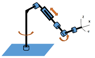
Horizontal movement corresponds to the x-axis or the y-axis. Thus, all gravitational forces can be easily described in the cartesian system. Robots with predominantly articulated arms are more suitable for work in constrained quarters than are the robots with cartesian configuration.

For example, the mounting capability of a jointed-arm mechanism in space is significantly better than that of a similar translational mechanism with a smaller number of building elements. This is a substantial advantage. A disadvantage lies in the fact that in the given design, the precision is reduced due to angular errors. Most often, the movement of the robot’s arms is rotational, which is why calculating the trajectory of the endpoint necessitates conversion into the polar system. In terms of mathematics, this is an isomorphic transformation from the real space described by cartesian coordinates into the real space described by spherical coordinates. The Jacobian determinant is a transformational element enabling conversion between the two systems.

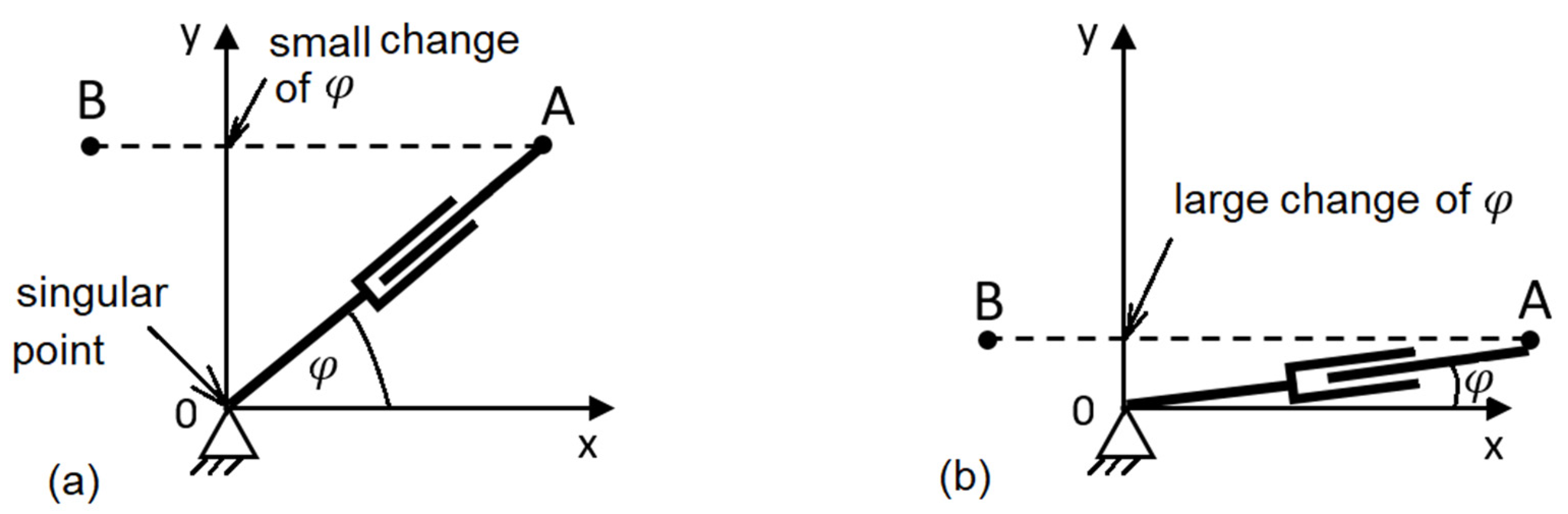
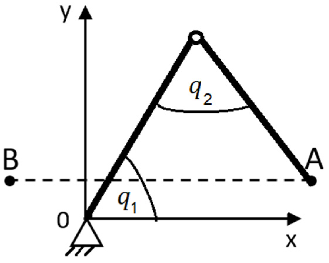
In the case of a planar telescopic arm anchored at the outset, the Jacobian determinant equals zero if the arm is reduced to zero (Figure 1). This state of inner singularity may materialize only if the required endpoint trajectory passes directly through the joint. Figure 1 shows a gradual worsening of the state dependent on the trajectory, which gradually approaches the joint. This example enables an illustrative observation of change in differential values in individual systems. It follows from the analysis of the movement that a small differential change of a parameter in the cartesian system corresponds to a large change in the polar system (Figure 1b). The inadequate step change of the angle occurs around the joint, where the movement portion under consideration, is the one always lying in the plane perpendicular to the joint’s axis.

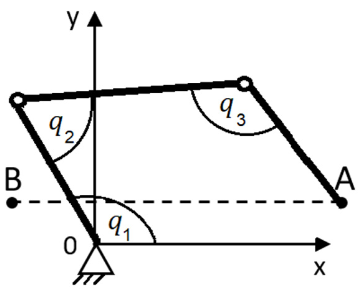
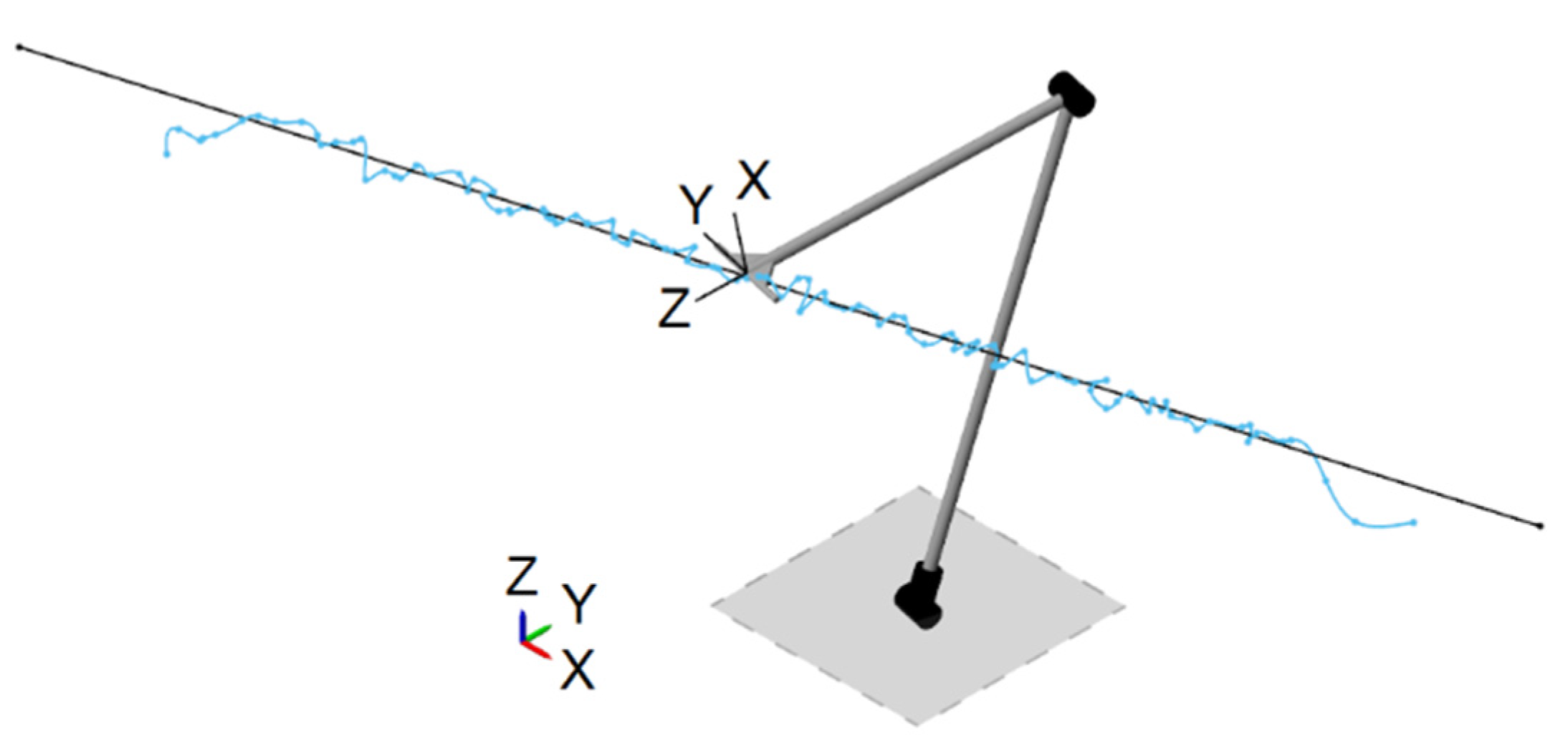
The same case will materialize if the mechanism in Figure 2 is used instead of a telescopic arm (Figure 2). Angle $\phi$ is replaced with a general parameter $q$ in line with the marking used in robotics.

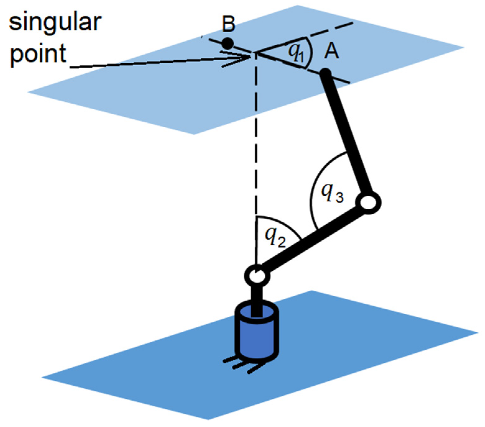
Drawing on the examples above, singularity may be avoided in two ways. The first way is that the trajectory of the endpoint mechanism will not pass in the vicinity of a singular state. The second way is that the robot’s redundant mechanism will be used. In the redundant mechanism case, the angular movements can be evenly distributed among all joints so that no singularity occurs in the movement across the joint’s axis (Figure 3).

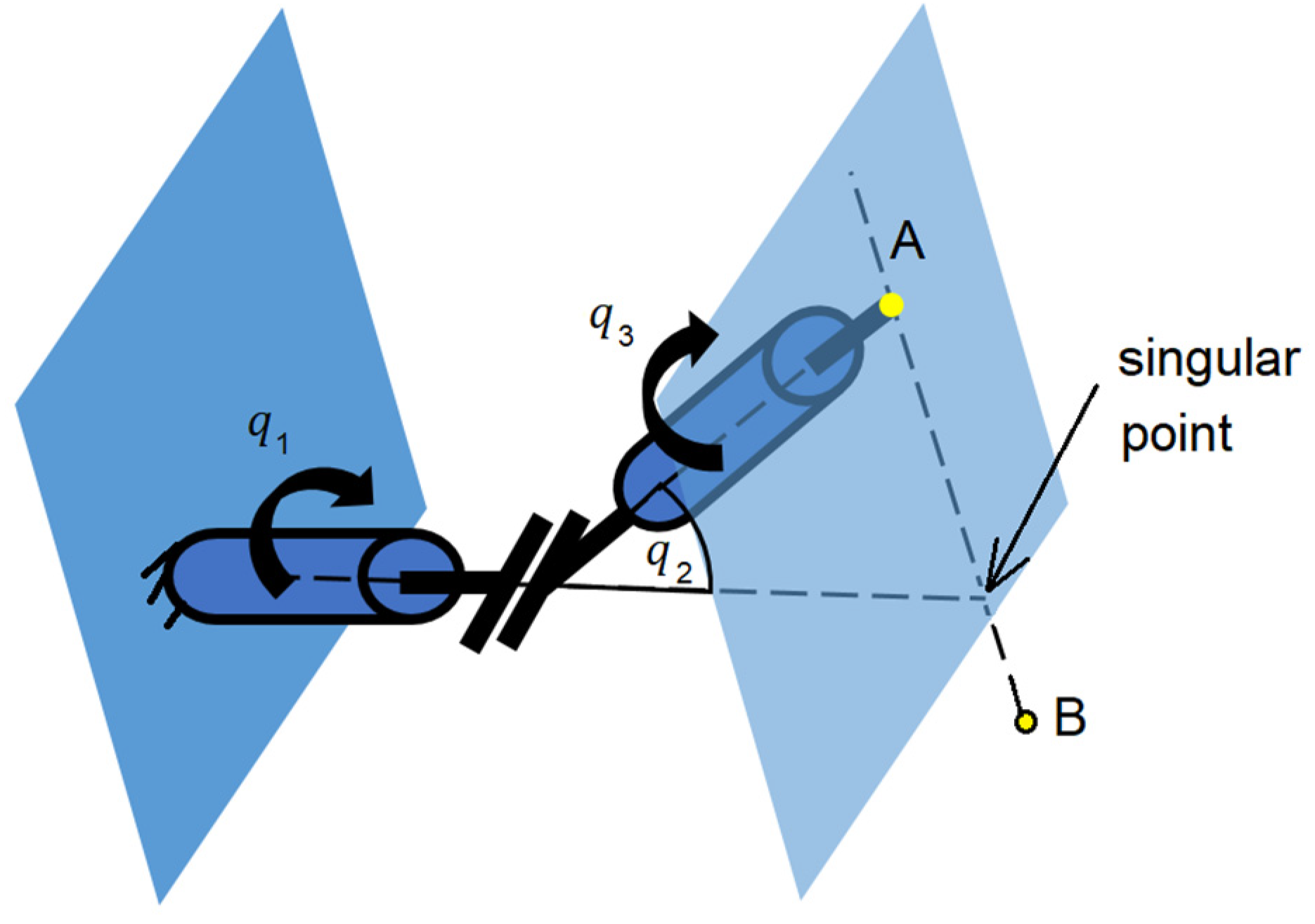
This principle of the inner singularity origin also holds for other types of known singular state designs. For example, a known arm singularity may be evaluated in the plane perpendicular to the axis of rotation (Figure 4). In principle, this state corresponds with the examples in Figure 1 and Figure 2.

By analogy, the wrist singularity, too, may be recognized on a similar principle (Figure 5).

The above examples make it clear that the principle of the origin of internal singularities is always the same:

“Inner singularity occurs in the case in which the nonredundant manipulator’s endpoint trajectory in a plane perpendicular to the axis of rotation passes through that axis”.

In reality, it is sufficient for the singularity to occur also when the movement is in close proximity to such a point. This fact may be beneficially taken advantage of in the analysis and detection of singular points in the robot’s workspace through the Monte Carlo method.

4. Application of the Monte Carlo Method to Assessing the Probability of Singular Points Occurrence

Input data for the identification of proximity of a singular point is the endpoint position with respect to the extended axes of the robot’s joints. The Monte Carlo method makes it possible to generate random positions of the robot arms’ configuration. Individual positions are generated based on an even distribution of the probability of occurrence in the given interval of movement. In such a case, each position has an equal chance of materializing. Each position can then be statistically evaluated in terms of attaining proximity to a singular state.

Surroundings of the singular point may be considered a critical area. The size of these surroundings is given by precision based on which a decision is made whether the Jacobian determinant will be considered to be quasi-zero. The agreed precision of calculation is, at the same time, a reference value for each mechanism type. If the critical value is exceeded, the point in the space this value refers to will be considered a singular point. 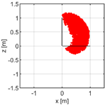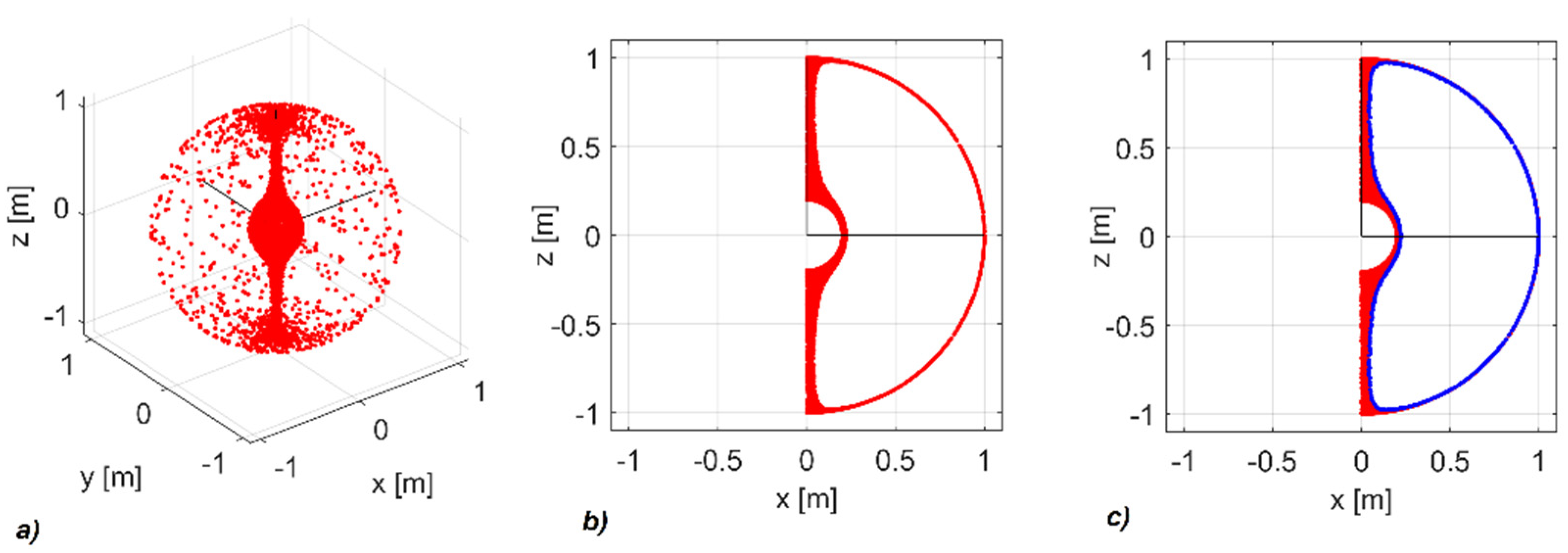Figure 6 shows the size of the area critical for singularity with respect to the workspace that originated through point generation for the telescopic mechanism (Figure 1). In this case, there is only one singular point, and its size represents the calculation precision of setting the Jacobian determinant with respect to the mechanism’s workspace. At the threshold precision value for calculating the Jacobian determinant of 0.01, the size of the tolerance field corresponds approximately to one-twentieth of the workspace span, which meets the simulation requirements.

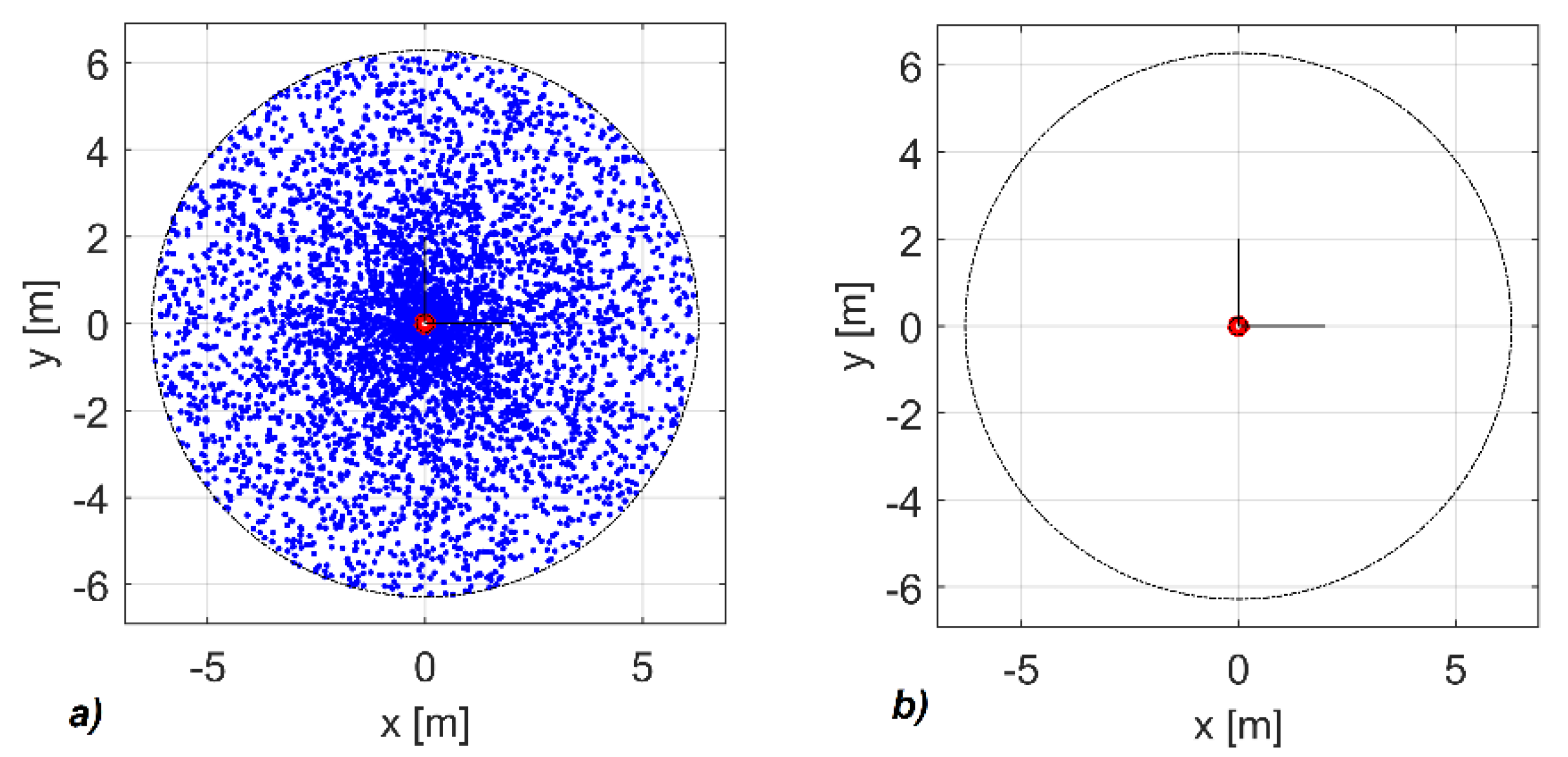
This precision has been maintained in all mechanisms. The mechanism with the revolute joints in Figure 2 has several singular points. The Monte Carlo analysis has yielded a map of singularities (Figure 7). Only outer singularities can be seen on the picture, as the second arm is shorter than the first one, so the kinematics of the mechanism does not allow the endpoint to pass through the central axis.

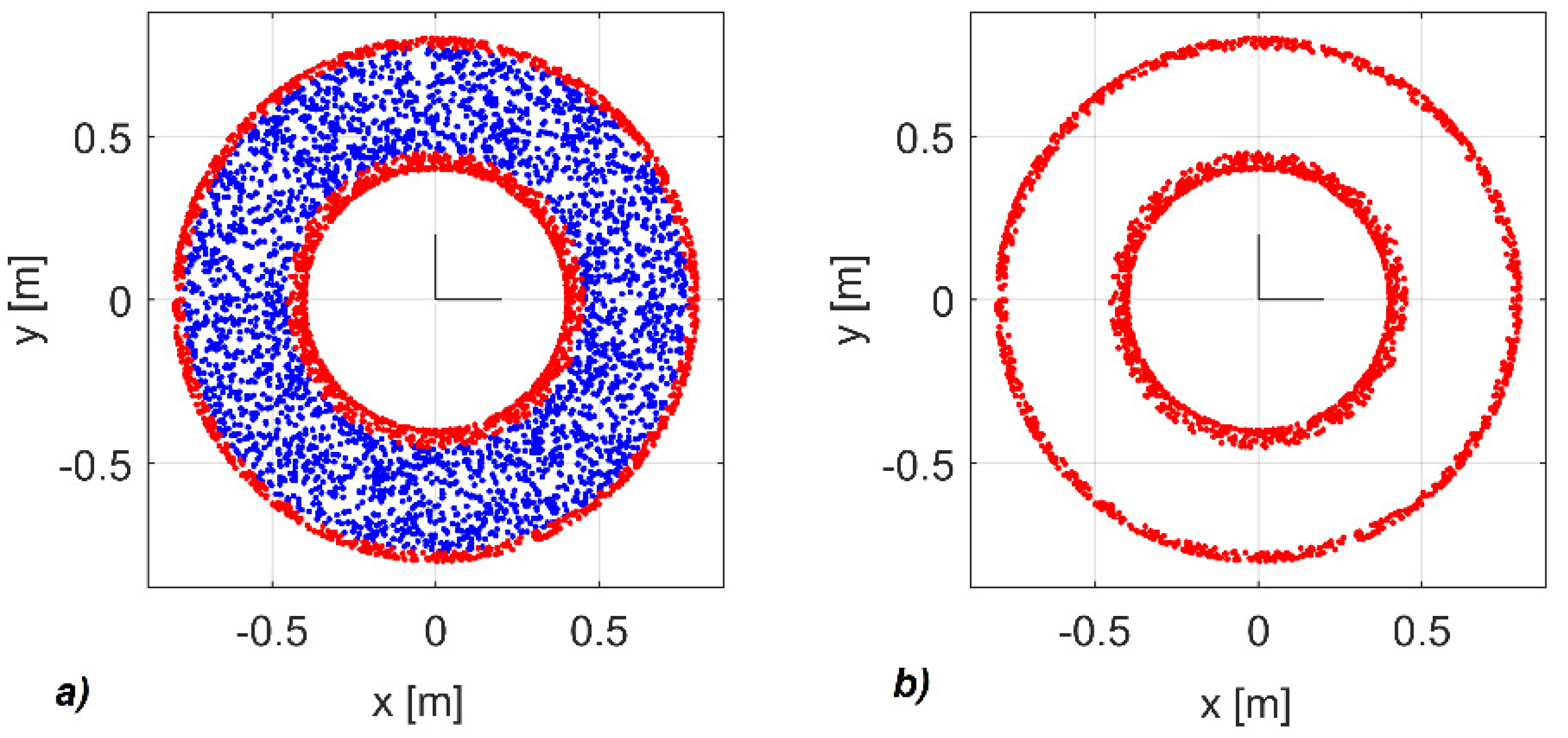
The generation of a large number of attempts will show the ratio and the distribution of the singular states versus the non-singular states. This is enabled by the visual rendering of the given workspace section. The distribution of singular points depends on the chosen size of tolerance of the Jacobian determinant and on the number of points generated. Figure 8 shows singular points in space, singular points in the planar section of the workspace, and pairs of singular and non-singular points. These pairs represent the mutual configuration of robotic arms that can be attained in several ways.

As the analysis has shown, a non-singular configuration can be attained in immediate proximity to singular points in all robot types. However, it needs to be decided here to what degree the established precision of calculating the Jacobian determinant is going to be critical for the given type of mechanism.

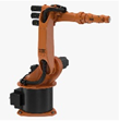
To compare the robots, two known designs (Stanford, Kuka) and one special design (URM-unlimited rotational module) have been selected (

Table 1. Maps of robots’ workspace singularities.

Robot	Kinematic Diagram	Singular Points	Mutual Configuration of Points
Stanford
Kuka
URM

).

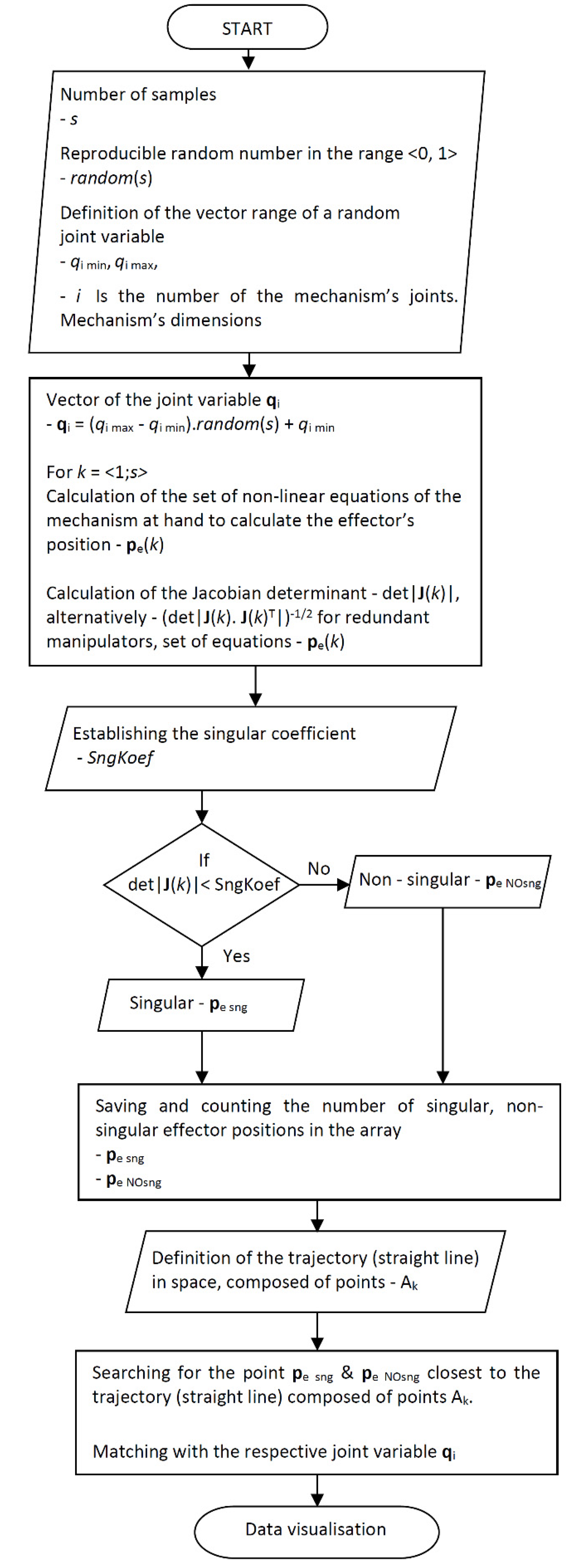
5. Algorithm That Determines Singular Points Generation

The input data for identifying proximity of a singular point are the endpoint position with respect to extended axes of the robot’s joints. Using the Monte Carlo method, random positions of the mechanism’s individual joints can be generated. The random number generator ensures an equal chance of attaining any particular configuration of the robotic arms. The output value is the position of the end effector (effector’s position) in 3D space. This position may be recorded in Matlab. At the same time, by calculating the respective Jacobian determinant, it is determined whether the generated point is singular or not. Figure 8 is an illustration of singular points for the mechanism in Figure 4.

Program from the flowchart (Figure 9) runs in Matlab. The input data are reproducible random joints variables with a certain number of samples. The precision value of determinant calculation det|J| is chosen to be 0.01 for all three mechanisms. For better rendering, the number of random samples is 50,000. The algorithm was used for the kinematics of the Kuka [28,29] robot mechanism, the Stanford mechanism [30,31] and the mechanism composed of the URM modules [4,32,33] (Table 1).

Variables:

s—Number of samples (indicates the number of samples generated)

random(s)—Reproducible random number (the Gauss distribution)

q_{i min}—Minimal value of a random joint variable

q_{i max}—Maximal value of a random joint variable

i—The number of the mechanism’s joints (degree of freedom)

q_i—The vector of the joint variable is the function of the sample—s, q_i(s)

k—Step of cycle

p_e(k)—End effector’s position

J(k)—Jacobian matrix

det|J(k)|—Jacobian determinant in its absolute value

SngKoef—Singular coefficient (any value in the range <0; 0.1>, in our case 0.01

singular state is assessed based on this value)

p_{e NOsng}—End effector’s position under non—singularity

p_{e sng}—End effector’s position under singularity

A_k—Points of the trajectory (straight line in our case) in space

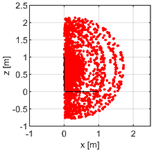
5.1. Singular Points Density Analysis

Due to its structure, a 3D chart is largely unclear. In addition, demands for the number of executed cycles grow. Since the mechanisms are of a radial symmetry around the z-axis, suitable rendering is that of the workspace diagonal section (Figure 8b). By making use of the Pythagorean theorem, the spatial points lying outside the section plane may be transferred inside the section plane. Rendering inside the workspace section requires fewer simulations to be generated. Such a section shows—beyond doubt—which areas are more singularity-prone. It goes without saying that the computational system would also work without transition in the cross-section. It would just take substantially longer. The majority of the mechanisms examined have radial symmetry.

The mutual configuration of the points has been obtained by comparing the critical distance of the singular and the non-singular point. If this distance is smaller in the analysis than the established critical value, then the workspace point in question may have both a singular and a non-singular configuration (Table 1). The analysis of a large number of points has shown that in all mechanisms each singular point has its non-singular counterpart. In other words, a singular point in the workspace may be approached in theory also through an infinitesimally close non-singular configuration of the robot’s arms (Figure 8c). However, this fact does not mean that these points can be attained through a smooth movement of robotic arms.

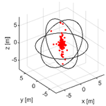
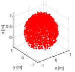
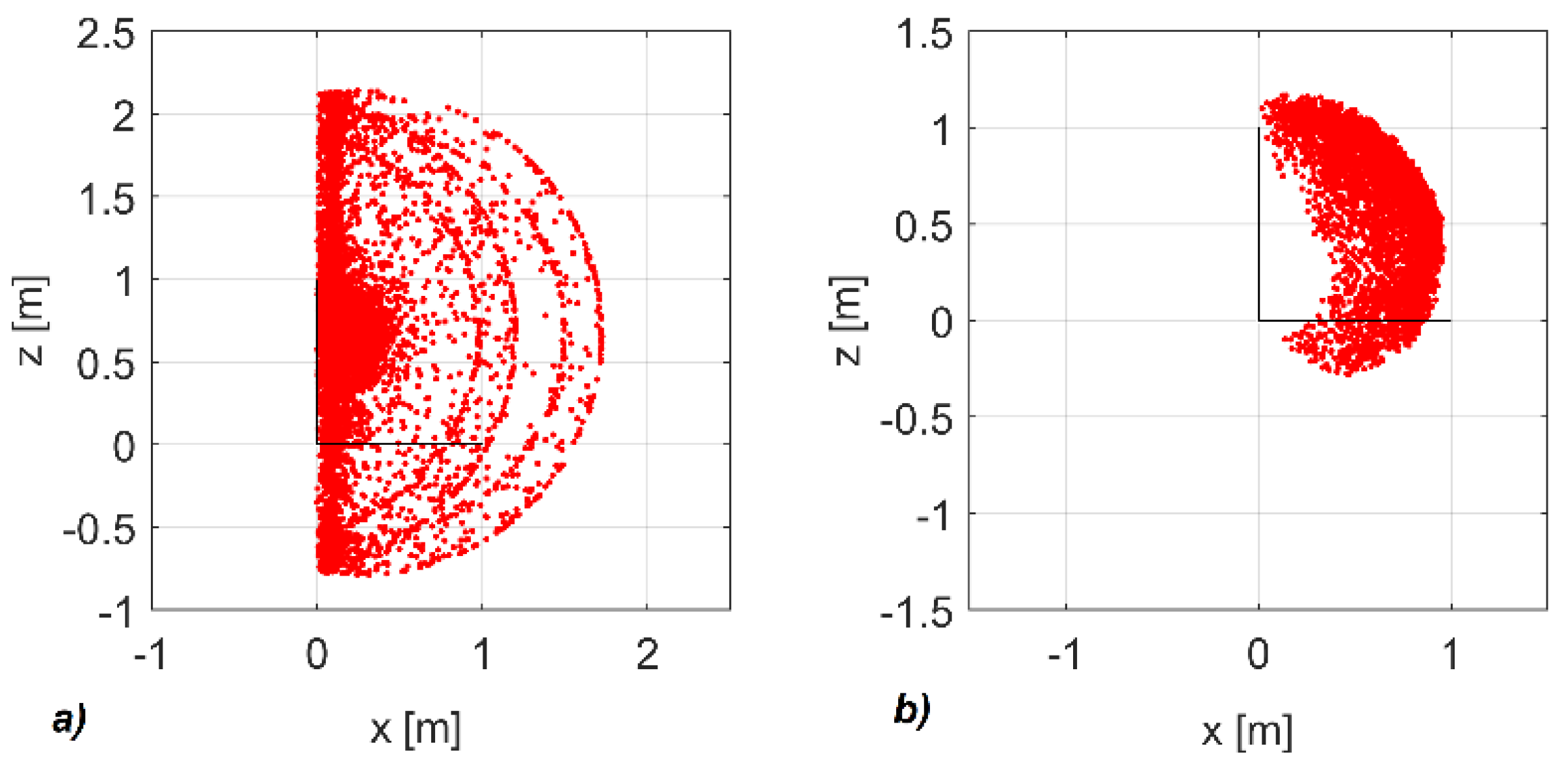
A greater informative value of the analysis is obtained from the density of the singular points’ distribution in space (Figure 10).

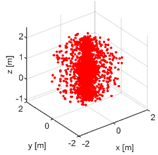
The Kuka robot displays fewer singular points (6575) at the selected number of samples compared to the URM (22450) robot. The point distribution in the case of Kuka robot is closer to the z-axis. In terms of programming, this distribution is more beneficial than an even points distribution in the URM robot’s case.

5.2. Analysis of the Configuration alongside Trajectory of the Endpoint Movement

The smoothness of the robotic arms’ movement was determined from a special analysis of the configuration along a straight line delimited by endpoints in the workspace. Individual A_k samples alongside the examined trajectory were ordered under the k index ranking. The essence of the analysis lies in the fact that a straight line or a line with a tolerance array was selected in the workspace. Only the non-singular points that fall within the straight line’s tolerance array in the Monte Carlo simulation are evaluated. The configuration of the angle parameters was saved for each of these points. When the points were ordered along the straight line, angle parameters can be rendered graphically.

Angular parameters are selected with a certain restriction on the movement of joints so as to reduce the number of possible configurations in a single trajectory point. This restriction may be adjusted to correspond to the existing real robot constraints. The constraints may be changed at will according to the analysis result. In this way, unambiguous solutions for the robot’s movement can be obtained and the computational time reduced.

The shape of the angle parameters determines the manner in which robotic arms may change from the initial point A to endpoint B in the course of the endpoint’s movement along the straight line. If the parameters change smoothly, such movement along the straight line is well-programmable. A smooth change means the angular changes between two adjacent points on the trajectory at the same robot configuration are small.

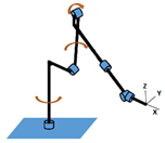
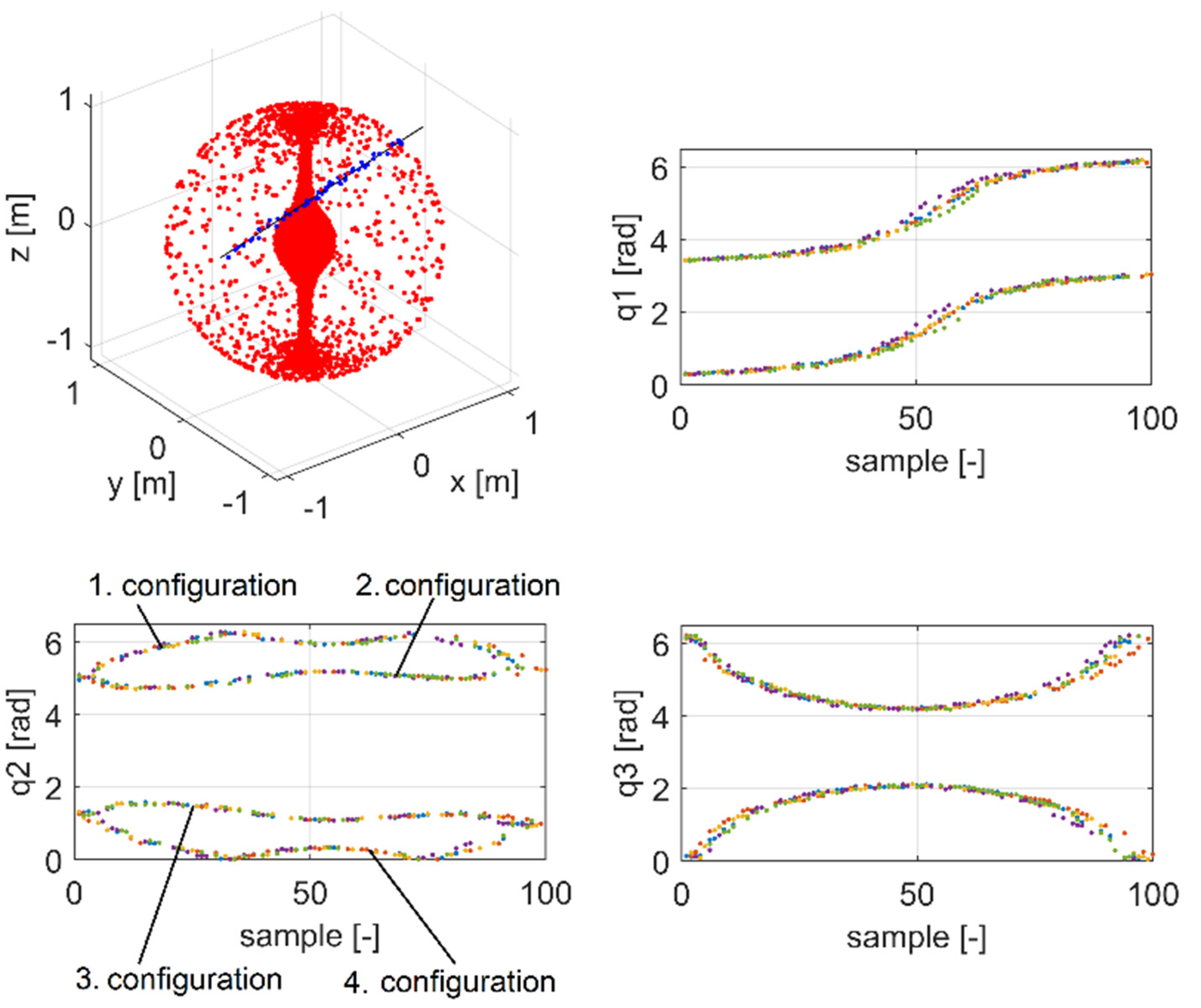
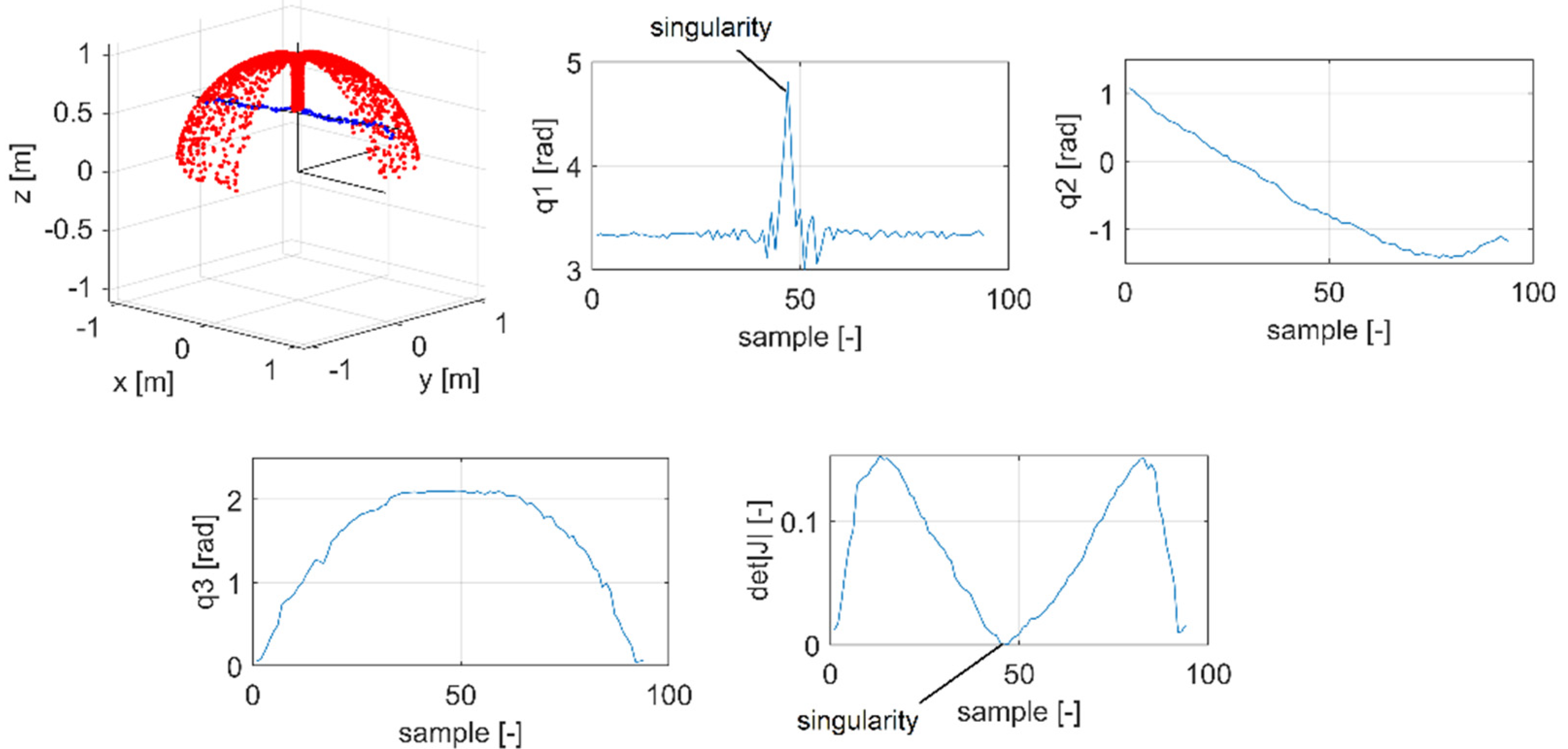
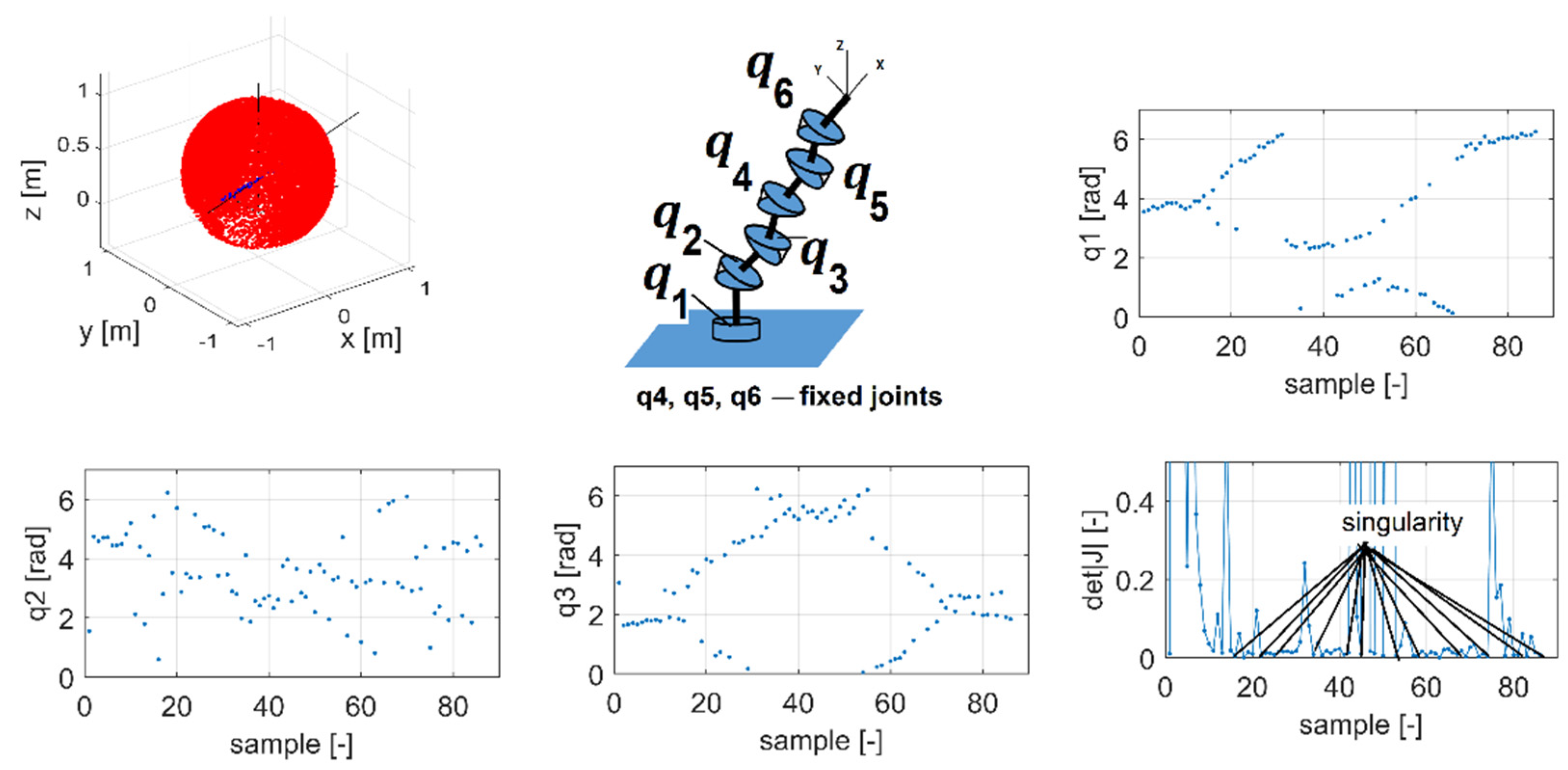
Figure 11 shows configurations with angle parameters along a straight line for a robotic mechanism featuring three joints (3 degrees of freedom) RRR in space (Figure 4). The analysis follows a point in space. In the case shown below, the system is non-redundant. A difference in the robot’s configuration is best seen in the change of the joint $q_2$.

Figure 12 shows spatial layout of the straight line and the mechanism in the coordinate system. Only one configuration of the robotic arm layout is shown out of four possible arrangements.

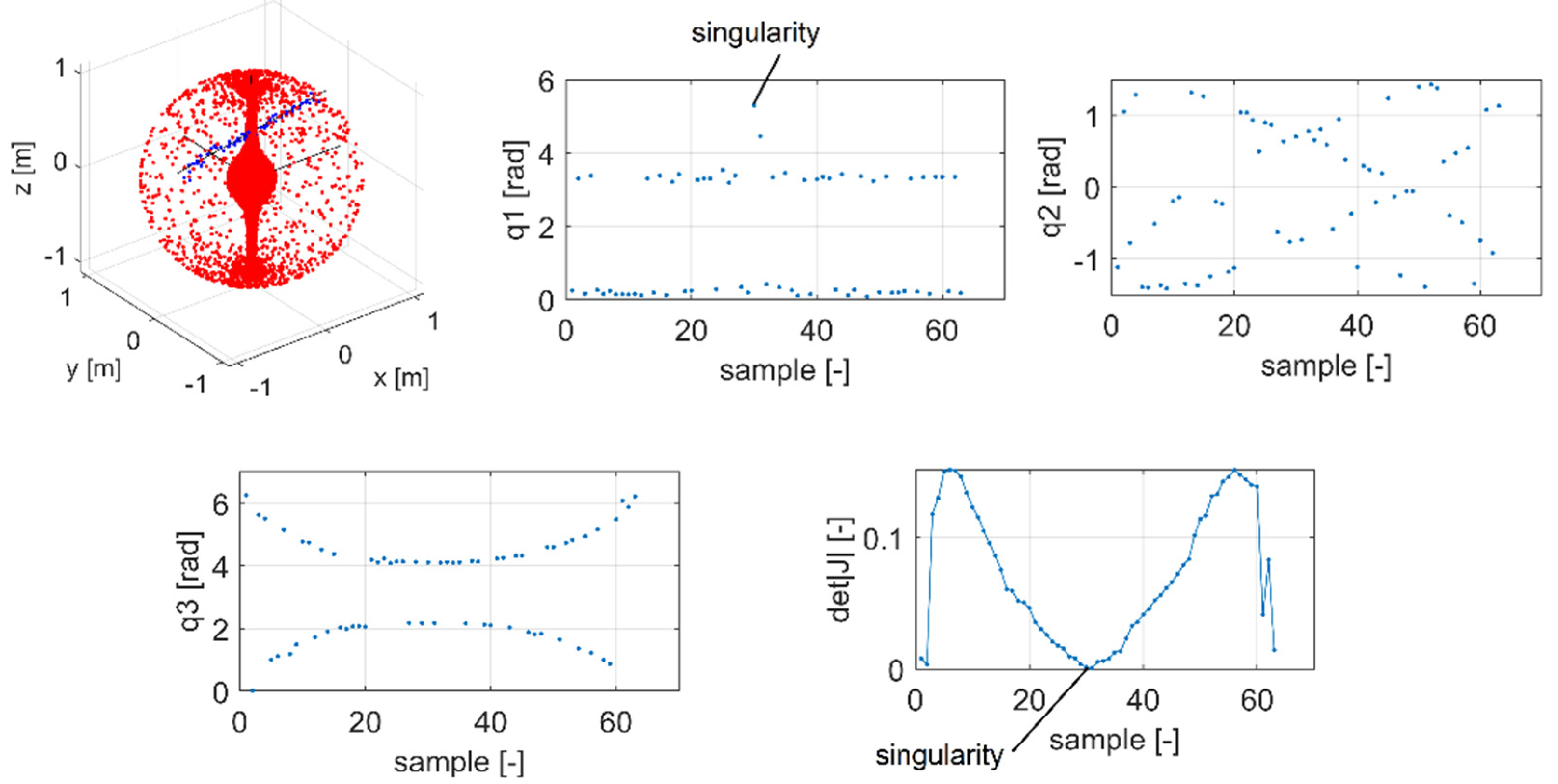
The analysis will change significantly if the straight line passes through a singular point in this mechanism, i.e., intersects the z-axis (Figure 13 and Figure 14).

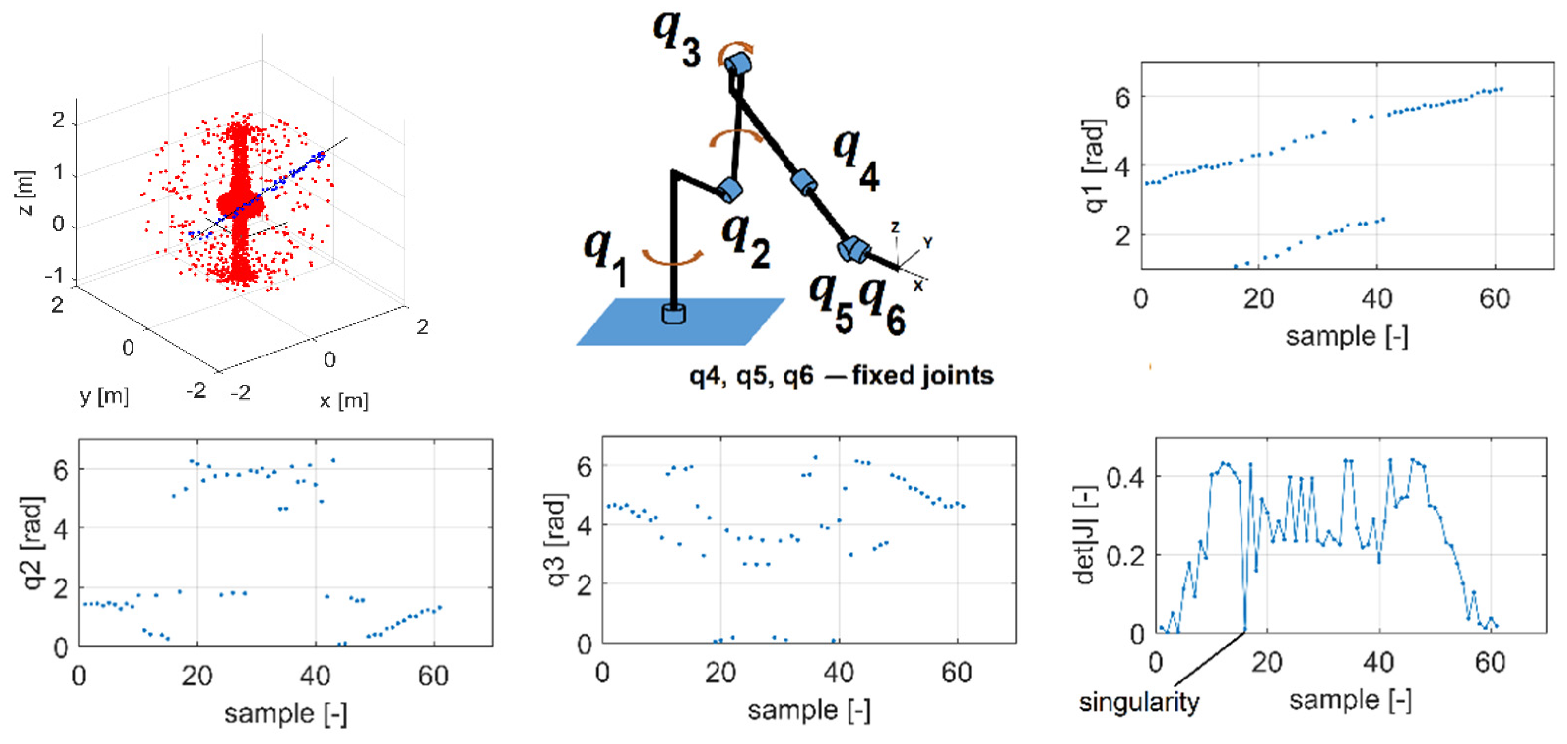
Analysis of the Kuka and URM robots’ workspace requires a certain configuration modification. A body in space has six degrees of freedom, to which the kinematics of non-redundant robots is adjusted. If only a single point is followed in space, three degrees are superfluous, and the system becomes redundant. Due to this, three angle parameters in the robots will be constrained, thus yielding a non-redundant system and the configuration with the remaining three parameters will be focused on. Practically, this is achieved by fixating the $q_4, q_5, q_6$ joints. This case concerns the end effector the orientation of which, with respect to the coordinate system, is the one mentioned above. The position of the straight line with respect to the Kuka robot workspace is shown in Figure 15. Conversely, Figure 16 shows a configuration of a robot composed of the URM modules.

As the analysis has shown, more singular points were found along the straight line of the URM than of the Kuka robot.

For the trajectory at hand, optimal solutions may be selected, where allowed, by limiting the values of the joint’s variables, thereby concentrating all samples on the movement around the trajectory. In such a case, no full revolution multiples ($\pm 360°$) of joints variables will occur, otherwise emerging from a wide range of joint variables’ parameters during random values generation. The entire computational power is thus focused on a particular solution, where a joint for the given trajectory does not have to move excessively, saving power needed to feed the drives as a result.

6. Conclusions

Analysis of different robots’ mechanisms singularities has shown substantial differences in distribution of singular points in the robot’s workspace. This is why the Monte Carlo analysis becomes yet another of the evaluation criteria for choosing the right robot to carry out work in the given technological operation. Of course, it is not the only criterion. The method does not, for example, reveal dynamic relations in maintaining the endpoint’s desired trajectory. There is, however, a general rule, saying the further away the endpoint moves from the singular point, the better the dynamic conditions of steering the moving elements. This can be suitably utilized with this method.

The Monte Carlo analysis along the trajectory offers the following benefits.

The benefits of the method lie in the fact that without calculating inverse kinematics, and with a sufficient number of samples, existing solutions to joint variables for the given trajectory can be established. If the system were a “black box” and we could measure the effector’s position in space, it would not be necessary to analyze even direct kinematics. Thus, constructing a singularities-free trajectory does not necessitate analytical solution.

This paper’s contribution lies in making the suitable selection of the joint variables more effective for the given configuration. The computational output focuses on achieving a greater solution precision over a shorter time.

Drawbacks of the method include prolonged and imprecise calculation when few samples for the given trajectory are available. Another disadvantage is the greater demands for computational speed (power) in finding precise solutions.

Mapping singularities with the Monte Carlo method is a computationally undemanding method with high effectivity of workspace rendering. A map obtained in this way supplies valuable information to robot work tasks programmers and planners. The optimal placement of a work object with respect to the coordinate system of the robot can be established quite clearly. In addition, suitable selection of robots for a particular work task in a particular workspace can be simulated and checked. This information can be obtained before a draft movement program is written for the robot under consideration.