
Quantum Compressive Sensing: Mathematical Machinery, Quantum Algorithms, and Quantum Circuitry

 ,
,  and
and 
Abstract
:1. Introduction
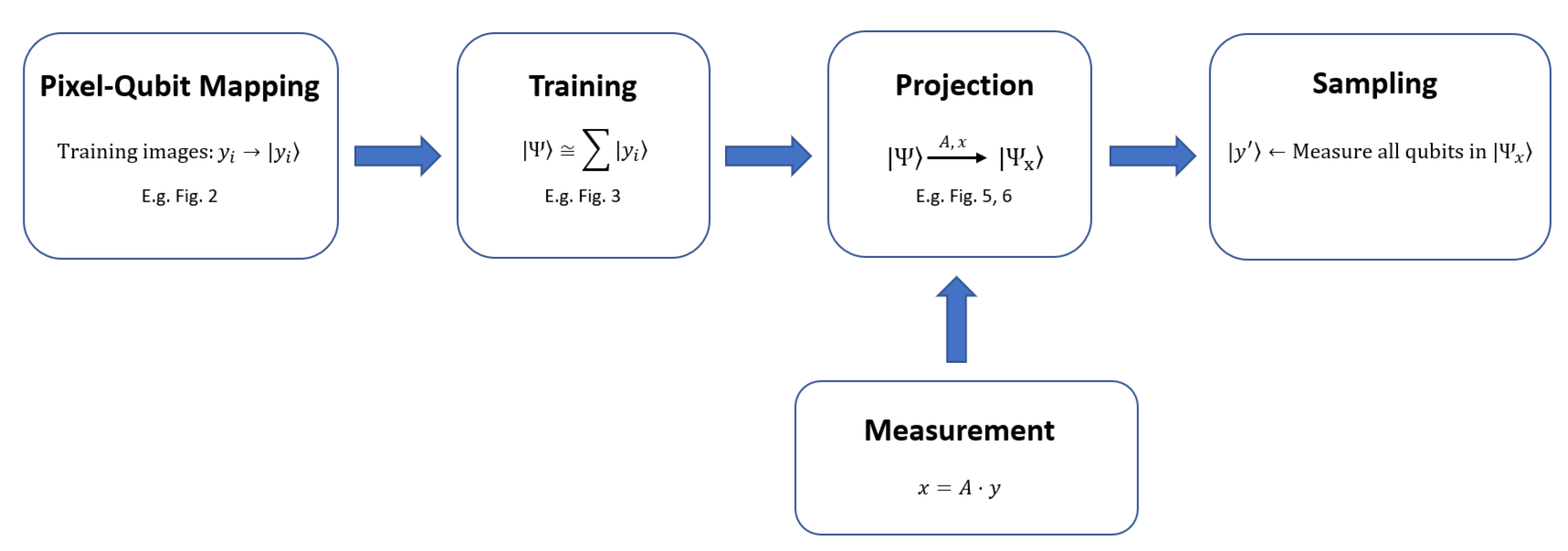
2. Quantum Compressive Sensing
- Training
- Measurement
- Projection
- Sampling
3. Pixel–Qubit Mapping
4. Training
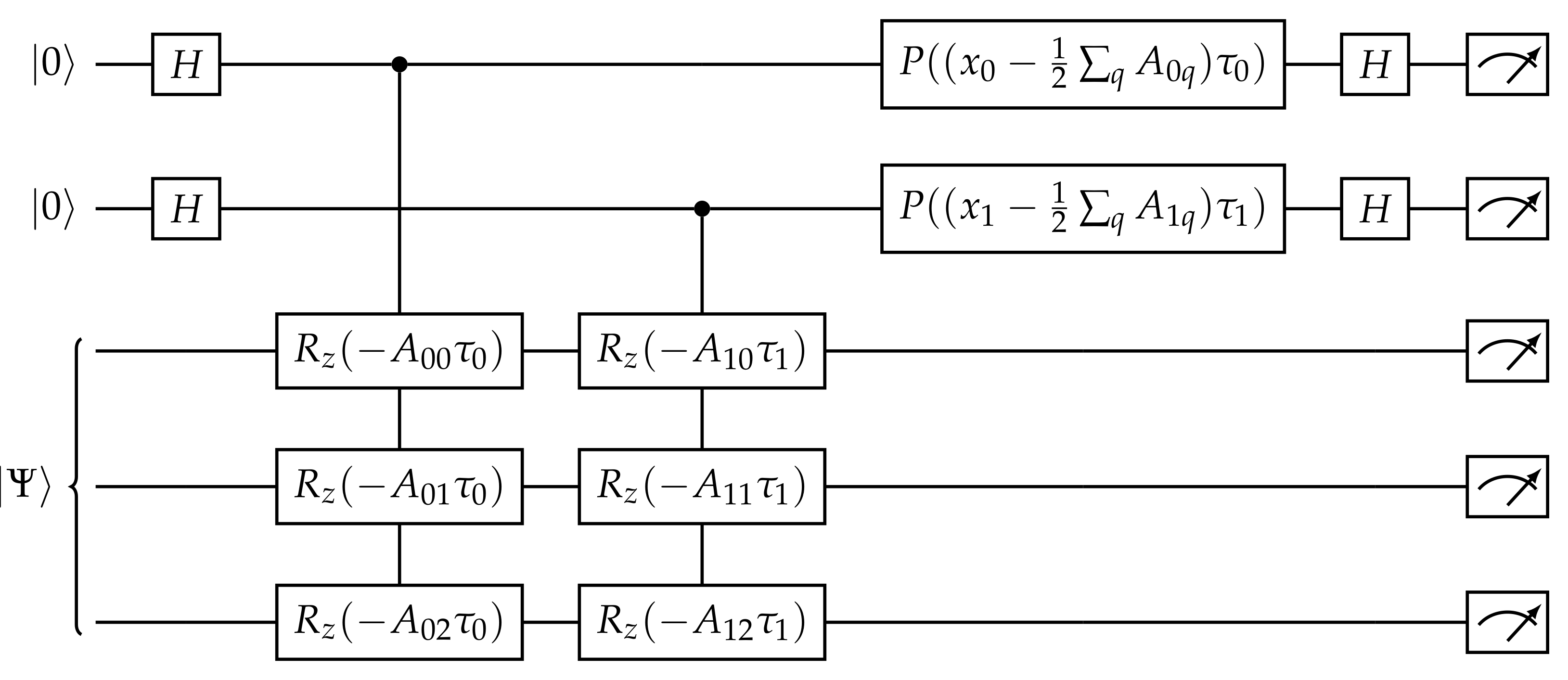
5. Projection
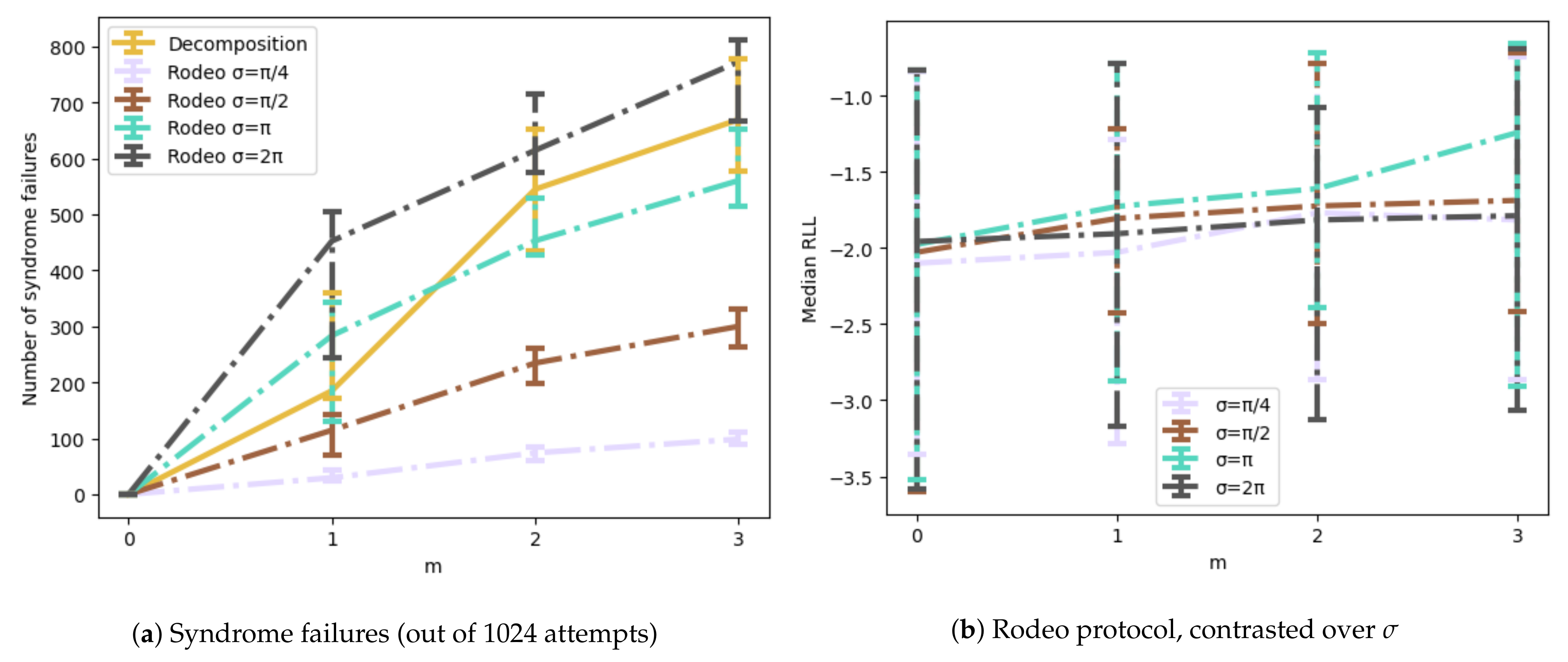
5.1. Decomposition
5.2. Rodeo Algorithm
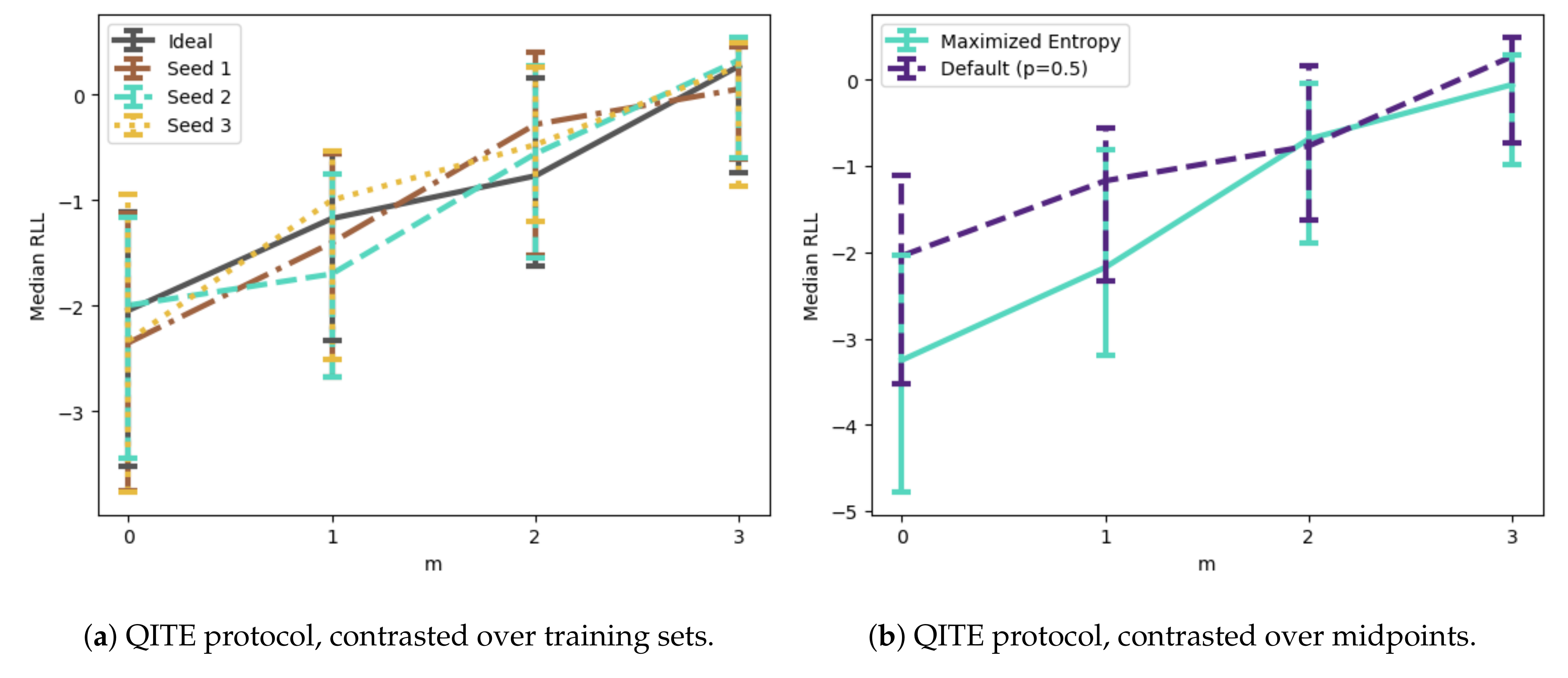
5.3. Quantum Imaginary Time Evolution
5.4. Entangled Born Machine
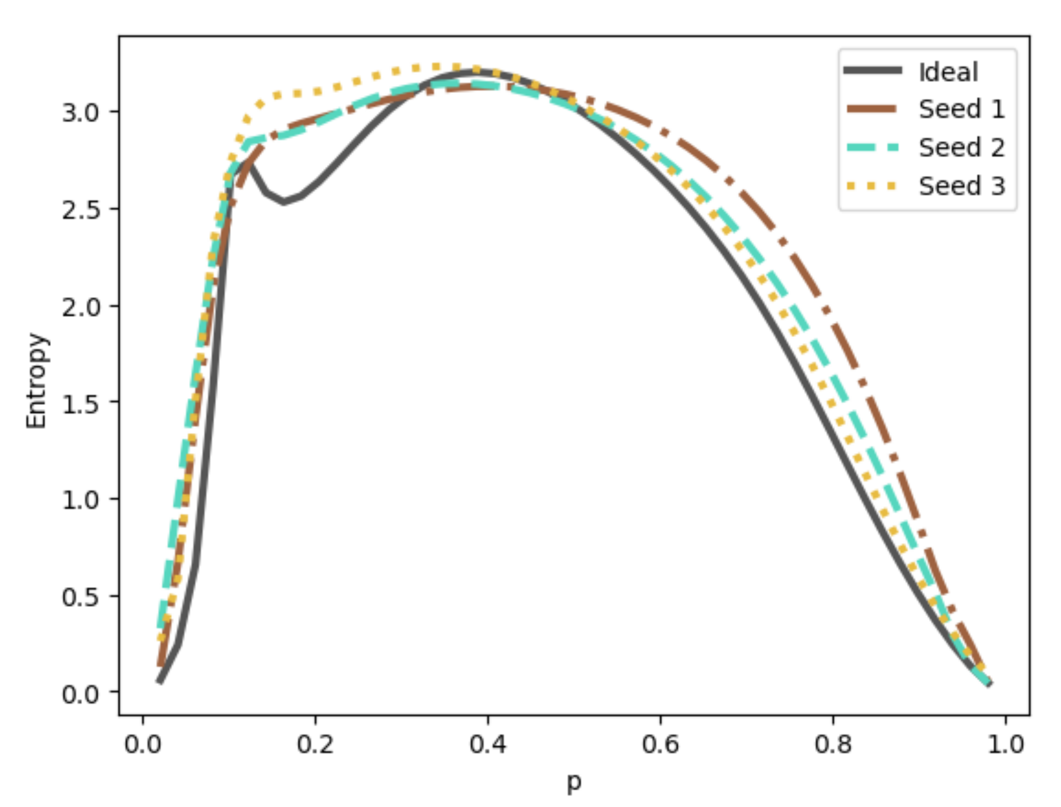
6. Demonstration
6.1. Description of Model
6.2. Quantum Compressive Sensing
7. Conclusions
Author Contributions
Funding
Institutional Review Board Statement
Informed Consent Statement
Data Availability Statement
Acknowledgments
Conflicts of Interest
Abbreviations
| MPS | Matrix Product State |
| TNCS | Tensor Network Compressed Sensing |
| LIDAR | Light Detection and Ranging |
| CASALS | Concurrent Artificially-Intelligent Spectrometry |
| NLL | Negative Log Likelihood |
| SVD | Singular-Value Decomposition |
| QITE | Quantum Imaginary Time Evolution |
| NISQ | Noisy Intermediate-Scale Quantum |
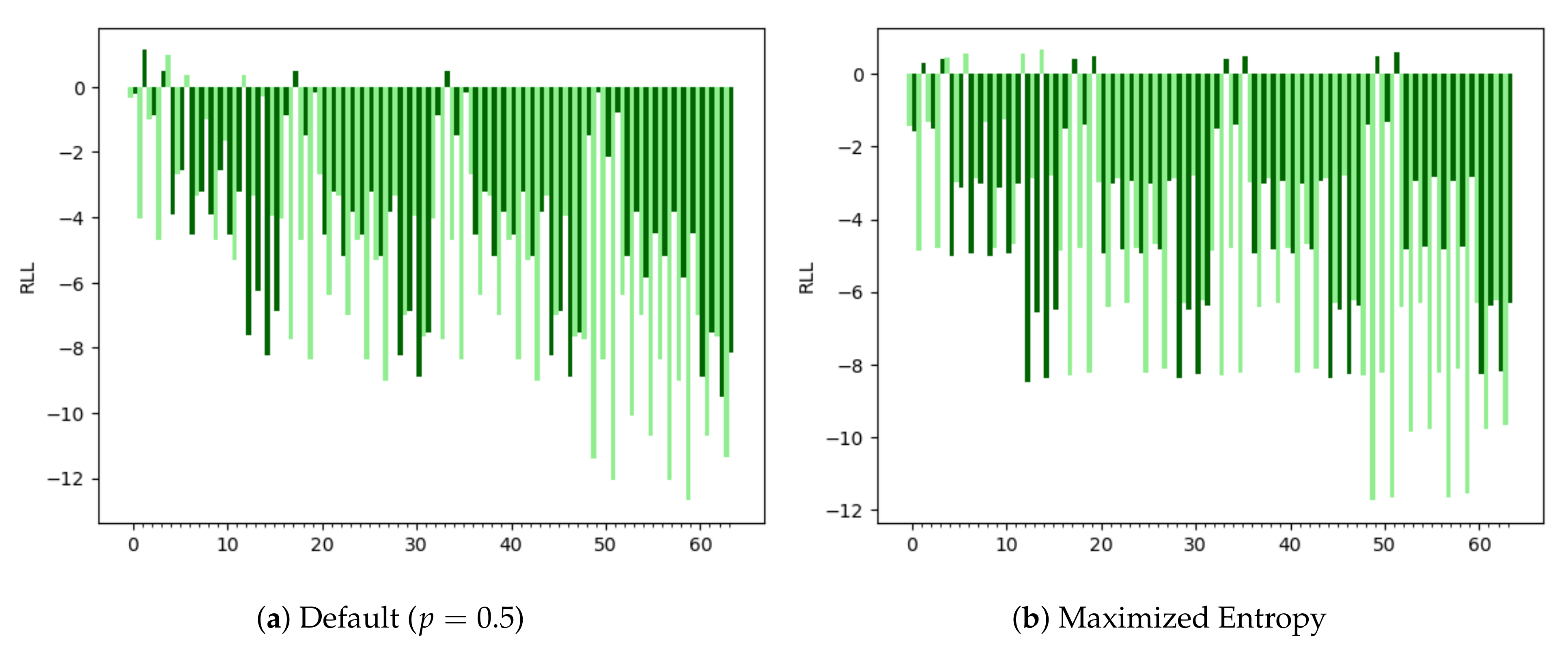
| RLL | Relative Log Likelihood |
Appendix A. Relative Log Likelihood
References
- Cheng, S.; Chen, J.; Wang, L. Information Perspective to Probabilistic Modeling: Boltzmann Machines versus Born Machines. Entropy 2018, 20, 583. [Google Scholar] [CrossRef] [PubMed] [Green Version]
- Liu, J.G.; Wang, L. Differentiable learning of quantum circuit Born machines. Phys. Rev. A 2018, 98, 062324. [Google Scholar] [CrossRef] [Green Version]
- Orús, R. Tensor networks for complex quantum systems. Nat. Rev. Phys. 2019, 1, 538–550. [Google Scholar] [CrossRef] [Green Version]
- Schollwöck, U. The density-matrix renormalization group in the age of matrix product states. Ann. Phys. 2011, 326, 96–192. [Google Scholar] [CrossRef] [Green Version]
- Stoudenmire, E.M.; Schwab, D.J. Supervised Learning with Quantum-Inspired Tensor Networks. arXiv 2016, arXiv:1605.05775. [Google Scholar]
- Han, Z.Y.; Wang, J.; Fan, H.; Wang, L.; Zhang, P. Unsupervised Generative Modeling Using Matrix Product States. Phys. Rev. X 2018, 8, 031012. [Google Scholar] [CrossRef] [Green Version]
- Ran, S.J.; Sun, Z.Z.; Fei, S.M.; Su, G.; Lewenstein, M. Tensor network compressed sensing with unsupervised machine learning. Phys. Rev. Res. 2020, 2, 033293. [Google Scholar] [CrossRef]
- Candes, E.; Romberg, J.; Tao, T. Robust uncertainty principles: Exact signal reconstruction from highly incomplete frequency information. IEEE Trans. Inf. Theory 2006, 52, 489–509. [Google Scholar] [CrossRef] [Green Version]
- Candes, E.J.; Tao, T. Near-Optimal Signal Recovery From Random Projections: Universal Encoding Strategies? IEEE Trans. Inf. Theory 2006, 52, 5406–5425. [Google Scholar] [CrossRef] [Green Version]
- Candès, E.; Romberg, J. Sparsity and incoherence in compressive sampling. Inverse Probl. 2007, 23, 969–985. [Google Scholar] [CrossRef] [Green Version]
- Candes, E.J.; Wakin, M.B. An introduction to compressive sampling: A sensing/sampling paradigm that goes against the common knowledge in data acquisition. IEEE Signal Process. Mag. 2008, 25, 21–30. [Google Scholar] [CrossRef]
- Candès, E.J. The restricted isometry property and its implications for compressed sensing. Comptes Rendus Math. 2008, 346, 589–592. [Google Scholar] [CrossRef]
- Baraniuk, R.G. Compressive Sensing [Lecture Notes]. IEEE Signal Process. Mag. 2007, 24, 118–121. [Google Scholar] [CrossRef]
- Chen, S.S.; Donoho, D.L.; Saunders, M.A. Atomic Decomposition by Basis Pursuit. SIAM J. Sci. Comput. 1998, 20, 33–61. [Google Scholar] [CrossRef]
- Candes, E.; Tao, T. The Dantzig selector: Statistical estimation when p is much larger than n. Ann. Stat. 2007, 35, 2313–2351. [Google Scholar] [CrossRef] [Green Version]
- Rudin, L.I.; Osher, S.; Fatemi, E. Nonlinear total variation based noise removal algorithms. Phys. D Nonlinear Phenom. 1992, 60, 259–268. [Google Scholar] [CrossRef]
- Osher, S.; Yin, W.; Goldfarb, D.; Xu, J. An Iterative Regularization Method for Total Variation-Based Image Restoration. Multiscale Model. Simul. 2005, 4, 460–489. [Google Scholar] [CrossRef]
- Osher, S.; Mao, Y.; Dong, B.; Yin, W. Fast Linearized Bregman Iteration for Compressive Sensing and Sparse Denoising. Commun. Math. Sci. 2011, 8, 93–111. [Google Scholar]
- Duarte, M.F.; Davenport, M.A.; Takbar, D.; Laska, J.N.; Sun, T.; Kelly, K.F.; Baraniuk, R.G. Single-pixel imaging via compressive sampling: Building simpler, smaller, and less-expensive digital cameras. IEEE Signal Process. Mag. 2008, 25, 83–91. [Google Scholar] [CrossRef] [Green Version]
- Howland, G.A.; Zerom, P.; Boyd, R.W.; Howell, J.C. Compressive sensing LIDAR for 3D imaging. In Proceedings of the CLEO: 2011—Laser Science to Photonic Applications, Baltimore, MD, USA, 1–6 May 2011; pp. 1–2. [Google Scholar] [CrossRef]
- Ouyang, B.; Dalgleish, F.R.; Caimi, F.M.; Giddings, T.E.; Shirron, J.J.; Vuorenkoski, A.K.; Nootz, G.; Britton, W.; Ramos, B. Underwater laser serial imaging using compressive sensing and digital mirror device. In Proceedings of the Laser Radar Technology and Applications XVI, Orlando, FL, USA, 27–29 April 2011; Volume 8037, pp. 67–77. [Google Scholar] [CrossRef]
- Bevacqua, M.T.; Crocco, L.; Di Donato, L.; Isernia, T. Microwave Imaging of Nonweak Targets via Compressive Sensing and Virtual Experiments. IEEE Antennas Wirel. Propag. Lett. 2015, 14, 1035–1038. [Google Scholar] [CrossRef]
- Wang, A.; Lin, F.; Jin, Z.; Xu, W. A Configurable Energy-Efficient Compressed Sensing Architecture With Its Application on Body Sensor Networks. IEEE Trans. Ind. Inform. 2016, 12, 15–27. [Google Scholar] [CrossRef]
- Liu, X.; Zhang, M.; Subei, B.; Richardson, A.G.; Lucas, T.H.; Van der Spiegel, J. The PennBMBI: Design of a General Purpose Wireless Brain-Machine-Brain Interface System. IEEE Trans. Biomed. Circuits Syst. 2015, 9, 248–258. [Google Scholar] [CrossRef]
- Kong, L.; Zhang, D.; He, Z.; Xiang, Q.; Wan, J.; Tao, M. Embracing big data with compressive sensing: A green approach in industrial wireless networks. IEEE Commun. Mag. 2016, 54, 53–59. [Google Scholar] [CrossRef]
- Colbourn, C.J.; Horsley, D.; McLean, C. Compressive Sensing Matrices and Hash Families. IEEE Trans. Commun. 2011, 59, 1840–1845. [Google Scholar] [CrossRef]
- Fay, R. Introducing the counter mode of operation to Compressed Sensing based encryption. Inf. Process. Lett. 2016, 116, 279–283. [Google Scholar] [CrossRef]
- Cerezo, M.; Sone, A.; Volkoff, T.; Cincio, L.; Coles, P.J. Cost function dependent barren plateaus in shallow parametrized quantum circuits. Nat. Commun. 2021, 12, 1791. [Google Scholar] [CrossRef]
- Bittel, L.; Kliesch, M. Training Variational Quantum Algorithms Is NP-Hard. Phys. Rev. Lett. 2021, 127, 120502. [Google Scholar] [CrossRef]
- Nielsen, M.A.; Chuang, I.; Grover, L.K. Quantum Computation and Quantum Information, 10th ed.; Cambridge University Press: Cambridge, MA, USA, 2002; Volume 70, pp. 558–559. [Google Scholar] [CrossRef] [Green Version]
- Jiang, Z.; Sung, K.J.; Kechedzhi, K.; Smelyanskiy, V.N.; Boixo, S. Quantum Algorithms to Simulate Many-Body Physics of Correlated Fermions. Phys. Rev. Appl. 2018, 9, 044036. [Google Scholar] [CrossRef] [Green Version]
- Choi, K.; Lee, D.; Bonitati, J.; Qian, Z.; Watkins, J. Rodeo algorithm for quantum computing. Phys. Rev. Lett. 2021, 127, 040505. [Google Scholar] [CrossRef]
- Motta, M.; Sun, C.; Tan, A.T.; O’Rourke, M.J.; Ye, E.; Minnich, A.J.; Brandão, F.G.; Chan, G.K.L. Determining eigenstates and thermal states on a quantum computer using quantum imaginary time evolution. Nat. Phys. 2020, 16, 205–210. [Google Scholar] [CrossRef] [Green Version]


Publisher’s Note: MDPI stays neutral with regard to jurisdictional claims in published maps and institutional affiliations. |
© 2022 by the authors. Licensee MDPI, Basel, Switzerland. This article is an open access article distributed under the terms and conditions of the Creative Commons Attribution (CC BY) license (https://creativecommons.org/licenses/by/4.0/).
Share and Cite
Sherbert, K.M.; Naimipour, N.; Safavi, H.; Shaw, H.C.; Soltanalian, M. Quantum Compressive Sensing: Mathematical Machinery, Quantum Algorithms, and Quantum Circuitry. Appl. Sci. 2022, 12, 7525. https://doi.org/10.3390/app12157525
Sherbert KM, Naimipour N, Safavi H, Shaw HC, Soltanalian M. Quantum Compressive Sensing: Mathematical Machinery, Quantum Algorithms, and Quantum Circuitry. Applied Sciences. 2022; 12(15):7525. https://doi.org/10.3390/app12157525
Chicago/Turabian StyleSherbert, Kyle M., Naveed Naimipour, Haleh Safavi, Harry C. Shaw, and Mojtaba Soltanalian. 2022. "Quantum Compressive Sensing: Mathematical Machinery, Quantum Algorithms, and Quantum Circuitry" Applied Sciences 12, no. 15: 7525. https://doi.org/10.3390/app12157525
APA StyleSherbert, K. M., Naimipour, N., Safavi, H., Shaw, H. C., & Soltanalian, M. (2022). Quantum Compressive Sensing: Mathematical Machinery, Quantum Algorithms, and Quantum Circuitry. Applied Sciences, 12(15), 7525. https://doi.org/10.3390/app12157525