Abstract
Unitary decomposition is a widely used method to map quantum algorithms to an arbitrary set of quantum gates. Efficient implementation of this decomposition allows for the translation of bigger unitary gates into elementary quantum operations, which is key to executing these algorithms on existing quantum computers. The decomposition can be used as an aggressive optimization method for the whole circuit, as well as to test part of an algorithm on a quantum accelerator. For the selection and implementation of the decomposition algorithm, perfect qubits are assumed. We base our decomposition technique on Quantum Shannon Decomposition, which generates controlled-not gates for an n-qubit input gate. In addition, we implement optimizations to take advantage of the potential underlying structure in the input or intermediate matrices, as well as to minimize the execution time of the decomposition. Comparing our implementation to Qubiter and the UniversalQCompiler (UQC), we show that our implementation generates circuits that are much shorter than those of Qubiter and not much longer than the UQC. At the same time, it is also up to 10 times as fast as Qubiter and about 500 times as fast as the UQC.
1. Introduction
Quantum computing is promising to provide the next phase of performance improvement for large-scale computing. To this end, many different algorithms have been developed in the theoretical domain, such as Shor’s algorithm for prime factorization in polynomial time [1], or Grover’s algorithm for finding a specific input corresponding to some output in time [2].
Recent years have seen some great strides in the field of physical implementations of quantum computers as well. However, these still have some big limitations on the number of qubits, the error rates and the length of the circuits that can be executed on them. Although quantum computers with as many as 128 qubits already exist [3], error rates are of the order – per gate [4]. Therefore, executing a circuit on a physical quantum chip requires significant error correction, as well as mapping, scheduling and other such measures [5].
These algorithms are executed on simulators, which come with their own set of restrictions. Some simulators require the use of specific qubit topology and limit possible qubit states or the number of qubits, and all of them are bound by the classical resources of the system the simulation is run on. The main resource limit is the memory necessary to store the quantum circuit and the total qubit state, which is dependent on the length of the circuit, the number of qubits and the degree of superposition. These also influence the processing time necessary to simulate the full circuit, which is generally done by some form of matrix multiplications of the qubit state and each gate in the circuit.
Unitary decomposition is the process of translating an arbitrary unitary gate (a unitary matrix U is a square, complex matrix, of which the inverse () and the conjugate transpose () are the same; i.e., and [6]) into a specific (universal) set of single and two-qubit gates. Unitary decomposition is necessary because it is not otherwise possible to execute an arbitrary quantum gate on either a simulator or quantum accelerator. This makes it a required feature for algorithms that use any type of gate that is not supported by the target platform or just produce an arbitrary unitary gate that will need to be translated. In this paper, only exact decomposition algorithms will be considered for application on gate-based quantum computing.
This paper proposes a highly-efficient method to implement unitary decomposition for quantum algorithms using Quantum Shannon Decomposition. The paper shows that our approach is up to 10× more efficient in terms of the number of gates generated for a given unitary matrix size and requires up to 100 times less wall-clock execution time than other implementations. The contributions of this paper are as follows:
- Implementation of Quantum Shannon Decomposition for the unitary decomposition of quantum algorithms;
- Decomposition optimizations that take advantage of the underlying matrix structure;
- The integration and evaluation of our method in the OpenQL quantum programming framework;
- The optimization of the implementation of a quantum genome analysis use-case using our method
This paper is structured as follows. In Section 2, applications for unitary decomposition are discussed. Then, in Section 3, some background is given on qubits, gate-based computation and the special qubit gates that are used. The specific decomposition method for multi-controlled gates is given in Section 4. In Section 5, several decomposition algorithms are compared based on their resulting CNOT-count. The implementation of the selected algorithm, Quantum Shannon Decomposition, is outlined in Section 6. Optimizations to this implementation can be found in Section 7. Experimental results are shown in Section 8 and compared to other implementations in Section 10. Finally, the conclusion and future work can be found in Section 11.
2. Motivation for Unitary Decomposition
Unitary decomposition is useful in several contexts. The first is the broad class of algorithms that generate arbitrary unitary gates that need to be translated into a quantum circuit, but it is also used to enable the more modular design of quantum algorithms or as an aggressive optimization method.
We will use two quantum algorithms that we have developed in the context of genome sequencing as an example of a possible application for unitary decomposition. With genome sequencing, a genome sequence is first read as many short pieces which then need to be combined to get the full DNA sequence. This is currently done using many different algorithms, which are executed using (classical) high-performance computing systems [7].
For genome sequencing using quantum accelerators, the DNA sequences can be stored in superposition. The two algorithms that will be discussed both use a unitary matrix in the process of finding the position of a short read (sequence of a small piece of DNA) on a reference genome. That matrix needs to be decomposed before the algorithm can be run on a quantum accelerator or simulator [8].
The first quantum genome sequencing algorithm we will use is Quantum Indexed Bidirectional Associative Memory (QiBAM) [8]. QiBAM uses a unitary oracle assembled from a binomial distribution as . Here, is a factor that influences the width of the distribution, is the Hamming distance between the query pattern p and all memory states x, and n is the number of qubits required to store the memory states. n is also the size of the vector and resulting matrix.
The second genome sequencing algorithm is Quantum Associative Memory (QAM). This uses a Hadamard-like transformation to store the patterns, assembled using Equation (1) [9].
In order to apply either gate from these two algorithms to qubits, they need to be translated into some combination of (elementary) quantum gates that can be executed on a quantum accelerator, and the same is true for other such algorithms.
Besides that, unitary decomposition also facilitates short-cuts in the design of new algorithms. With unitary decomposition, a developer can keep part of an algorithm as a unitary gate/matrix while working on some other part and test this. Otherwise, the algorithm can only be executed in full when all of it is made out of known quantum gates. Unitary decomposition allows the full algorithm to be tested and checked much earlier in the development process on the target quantum chip or simulator.
Furthermore, unitary decomposition can be used as an aggressive optimization method, because the maximum number of gates resulting from a decomposition can be calculated easily beforehand. The maximum length of the circuit resulting from the decomposition is only dependent on the number of qubits affected by the gate. For circuits longer than this maximum, and thus consisting of more gates, the assembly of all gates into a unitary matrix and then decomposing that matrix will always result in a shorter circuit.
Someone programming in OpenQL might, for example, specify a circuit with three qubits with 180 gates—this might be because of application semantics, code-readability or because they did not consider the optimal way to program their quantum algorithm. The total of 180 gates is more than the number of gates that would result from decomposing an arbitrary three-qubit gate. Thus, if the circuit is combined into a single unitary matrix and then that matrix is decomposed using Shannon Decomposition, for example, then the length of the circuit will be reduced from 180 gates to only 120 (84 rotation gates and 36 CNOT gates).
Something to consider, however, is that the circuit resulting from the decomposition of a unitary matrix is longer than the theoretical minimum, and even the theoretical minimum number of gates for a general n-qubit unitary gate becomes quite large very quickly, since it scales with in the leading term. Thus, in most cases, a hand-optimized and application-specific circuit will be shorter than the one resulting from universal unitary decomposition. However, these hand-optimized circuits are labor-intensive and require a significant amount of time to develop, while unitary decomposition can be done automatically.
3. Background
In this section, the background and notations are given for qubits, quantum gates, unitary matrices, the universal set of gates that are used, quantum multiplexers and multi-controlled gates.
3.1. Qubit Notation
A qubit state is represented in bracket notation as
Besides the notation, quantum states can also be represented as complex vectors: . This is especially useful for the combined state of multiple qubits, where the first row of the vector corresponds to the binary number “0” in as many bits as there are qubits. The second row corresponds to the number “1”, etc. As an example, for a three-qubit state, the first row corresponds to , and the second to . This continues to the final row, which is . The state vector has rows for the state of n qubits.
3.2. Quantum Gates
Qubits are manipulated using gates, which are matrices that operate on the qubit state vector. To calculate the effect of gates on the combined qubit state, the state vector is multiplied by the matrix representations of the gates in reverse order.
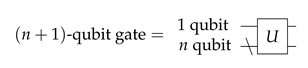
In the circuit notation, each line going into or out of a gate represents one qubit. To represent n-qubit gates—gates that affect an unspecified number of qubits—a line with a backslash through it is used.
3.3. Unitary Matrices
A reversible quantum gate acting on n perfect qubits can be fully described as unitary matrix [10]. The set of unitary matrices of size by is written as and has the following properties [6]:
- ;
- U is diagonalizable;
- has a set of orthogonal eigenvectors;
- For a unitary matrix , .
The Special Unitary group, , is a subgroup of unitary matrices where
- for U in [11].
When a measurement is performed, the global phase () of the qubits does not influence the measurement probabilities. This means that all quantum gate operations can be represented by a matrix in [12]. These properties are used to decompose the matrix, using one of the algorithms described in Section 5.
3.4. Universal Set of Gates
In order to decompose all possible unitary matrices into quantum gates, a universal gate set is selected as CNOT, the and gates. These three were selected because they are used in most decomposition methods.
3.5. Quantum Multiplexers
Besides these conventional gates, there are several gates used in this paper as intermediate results for the various decomposition algorithms. The first is the quantum multiplexer, which corresponds to a unitary matrix corresponding to the following structure Equation (3).
where denotes a unitary gate over n qubits, which is a unitary matrix of rows and columns. and are both ()-qubit gates. The rest of the matrix of U is zero. The gate is uniformly controlled, which means that when the control is 0, the upper left () of the matrix affects the qubits. However, when the control is 1, the lower right gate () is applied. The circuit for this is shown in Figure 1.
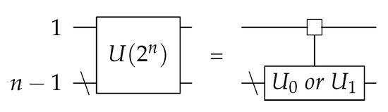
Figure 1.
A quantum multiplexer.
The first line is the controlling qubit, and the lower line is the rest () of the qubits. The box with the line to the lower gate means that it is uniformly controlled.
3.6. Multi-Controlled (Rotation) Gates
Another common intermediate gate is the multi-controlled (rotation) gate. This is a one-qubit gate with k control bits. Rather than just applying a gate when all control bits are zero, the applied operation to the target qubit can be different for each of the possible classical values of the control qubits.
This is written as , which is a fully or multi-controlled U(2) gate with k control qubits, with the target qubit at position m. The circuit representation of this gate is shown in Figure 2. To indicate that an operation is applied for either state of the control bits, a square control box is used.
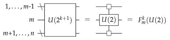
Figure 2.
A multi-controlled U(2) gate.
These multi-controlled gates correspond to a (block) diagonal unitary matrix, which is why they show up frequently in decomposition schemes. This is shown in Equation (4).
A multi-controlled rotation gate around axis a corresponds to the matrix shown in Equation (5). This can be any axis, but in the paper, the multi-controlled and axes are mainly used.
4. Decomposing Multi-Controlled Rotation Gates
The multi-controlled rotation gates from Section 3.6 can be decomposed into a combination of CNOTs and regular rotation gates. This can be done using the method from [13], which results in CNOTs gates and 1-qubit rotation gates for a controlled rotation gate with k control bits. To move from an -gate to an -gate, a circuit such as Figure 3 can be used.
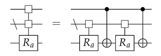
Figure 3.
Partial decomposition of an -gate.
This can be extended until only CNOT gates and one-qubit rotation gates are left, which leads to an example decomposition of a rotation gate with three control bits as shown in Figure 4.
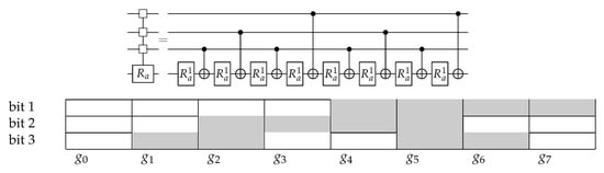
Figure 4.
Decomposition of an -gate.
To directly calculate which qubit is the control bit for each CNOT, this can be determined using Gray code. This is shown in the table below the circuit. The number of the bit that is changed in the Gray code is the number of the qubit that will be the control bit.
For each control bit of the multi-controlled gate, a one-qubit rotation gate and a single CNOT is used, so the total decomposition of an -gate requires rotation gates and CNOTs [13]. This is the least-known number of gates for decomposing such a matrix and is therefore used in almost all decomposition methods for (block) diagonal matrices of this form.
5. Comparison of Different Decomposition Methods
In this section, first, the selection criteria for the various decomposition methods is outlined in Section 5.1. Then, the theoretical lower bounds for the number of gates resulting from decomposition are given in Section 5.2, with implementations for a one and two-qubit gate in Section 5.3 and Section 5.4. This is followed by an examination of various general decomposition methods from the literature in Section 5.5, Section 5.6, Section 5.7 and finally the selection in Section 5.8.
5.1. Selection Criteria
Quantum computers are currently limited by the error rates and decoherence of qubits [4], and the longer the circuit, the higher the chance of errors will become. Therefore, the selection is based on circuit length, although the decomposition algorithm is only tested with perfect qubits on a simulator for now. In accordance with the motivations laid out in Section 2, only exact decomposition algorithms are considered.
For all decomposition methods, the number of gates resulting from the decomposition is only dependent on the number of qubits affected by the unitary gate. Thus, for generic n-qubit unitary gates, the resulting circuit length can be calculated from the size of the input matrix.
To measure the length of the resulting circuit, the number of CNOT gates will be used. There are several reasons for that. The first is that not all papers distinguish between generic one-qubit gates and rotation gates. The decomposition of a generic one-qubit gate takes three rotation gates (see Section 5.3), so the comparison might be a factor of three off if one-qubit gates are used to judge circuit length. The CNOT gate is used as the result for all decomposition methods and always has the same definition. This makes it a good metric for the total circuit length.
Secondly, each CNOT can generate entangled states between qubits [14], and for execution of the circuit on (near-term) quantum devices, each CNOT between non-neighboring qubits might introduce additional mapping operations [5]. Thus, to reduce mapping in the future, a circuit with as few CNOTs as possible is desired.
Thirdly, the error-rates for two-qubit gates are currently considerably higher than for one-qubit gates [4]. Thus, the chance that an error occurs in a circuit becomes much bigger with more CNOTs. Thus, to make the decomposition feasible for near-term quantum applications, it is not only important to keep the circuit-length low but especially the CNOT count.
5.2. Theoretical Lower Bounds
There is a theoretical lower bound for the number of CNOTs resulting from the decomposition of an n-qubit gate, and it is mathematically proven to be [15]. There are implementations that reach this number for one and two-qubit gates [15], as outlined in the next sections. This lower limit is included in the comparison, because it is useful to keep in mind what is and is not possible in terms of algorithms for unitary decomposition.
5.3. ZYZ Decomposition
For a one-qubit gate, no CNOT gates are necessary, and if rotation gates around any axis are possible, only one such gate is needed to apply any one-qubit operation. However, when using standard elementary gates, such as rotations around the Pauli X, Y or Z-axis, the decomposition of an arbitrary one-qubit gate results in three rotation gates using ZYZ decomposition [15].
One way to do this is with two rotation-z gates and one rotation-y gate. For this decomposition, the angles can be found so that the following equation is satisfied:
These angles can be calculated using the eigenvalues of the matrix and are used in the circuit shown in Figure 5. This is a universal decomposition for a one-qubit gate [15].
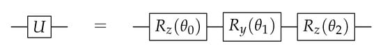
Figure 5.
Minimal universal quantum circuit for a one-qubit gate [15].
5.4. Minimal Decomposition of Two-Qubit Gates
From the theoretical lower bounds, we know that at least 2.25 CNOT gates are needed for a two-qubit gate. This rounds up to three CNOTs, and a circuit that achieves that number is shown in Figure 6 [15].
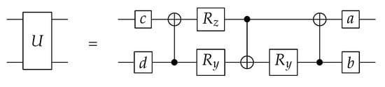
Figure 6.
Minimal universal quantum circuit for a two-qubit gate using 18 elementary gates [15].
To obtain the values for the gates of this circuit, first angles , and are found as in the ZYZ decomposition (Section 5.3). These are used to make circuit v so that the following holds:
The circuit v is shown in Figure 7.
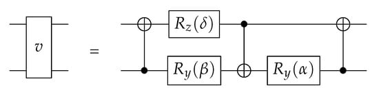
Figure 7.
The circuit v used to construct a universal two-qubit gate [15].
Then, to get the one-qubit gates, first matrix can be found so that is diagonal ( is the special orthogonal group, which means that the inverse of a matrix Q is equal to its transpose: and ). Through more diagonalization, can be found so and matrix C as . This leads to , and because A, B and C are in the special orthogonal group, they can be implemented by two unitary gates. After combining and B, the four gates can be found as [15]
which gives the circuit in Figure 6. The four one-qubit gates can be implemented by three rotation gates each, through ZYZ decomposition, so that the total rotation count is and the total CNOT count is just the ones for the circuit v, and thus three. This matches the theoretical lower bounds for an arbitrary two-qubit gate.
5.5. Decomposition with Givens Rotations
In [16] a method of decomposition is described that uses the Givens rotation matrices to perform the QR factorization of a unitary matrix. Each Givens rotation nullifies the element on the ith column and jth row of a matrix, as
The modified elements of U are indicated with a tilde, and the element on the lower left is nullified by the Givens rotation. Each Givens rotation matrix is equal to the identity matrix except for and for the elements at positions , , and , with the angle of the Givens rotation. These are to nullify elements until all elements below the diagonal are zero, at which point the following equality holds [16]:
By reordering the base vectors according to Gray code (see Section 3.6), the cosine and sine elements will all be adjacent. This is convenient for quantum computation, because that means that each Givens rotation matrix can be implemented by a controlled one-qubit gate, , with k control bits. For one specific combined state of the control qubits, the gate is applied to qubit i, while for all other states, the target qubit is left unaffected. This means that
where denotes the ith number of the Gray code, and the gates are formed from the matrix for the Givens rotations. This results in the circuit shown in Figure 8 for the decomposition of a twp-qubit gate.
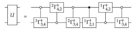
Figure 8.
Decomposition into the Givens rotations [16].
The numbers of elementary gates and CNOTs were calculated using [17], which are the numbers included in the table. Generally, this decomposition requires approximately controlled gates, which follows from a recursive relation of [16].
5.6. Recursive Cosine Sine Decomposition
With the circuit presented in [18], an n-qubit gate is decomposed into multi-controlled rotation gates. Cosine sine decomposition (CSD) is applied recursively until all the matrices are diagonal.
With CSD, any even-dimensional unitary matrix U can be decomposed into real diagonal matrices C and S and smaller unitary matrices , , and as shown in Equation (15) [19].
The left and right matrices are uniformly controlled gates; see Section 3.5. C and S are diagonal matrices with the cosines and sines of angles as the diagonal elements, respectively, between the subspaces, as shown in Equations (16) and (17).
where the values are ordered from large to small and are between and 0.
The central matrices from each recursive step correspond to multi-controlled gates which are decomposed as in Section 3.6. The other diagonal gates can be decomposed into a circuit consisting of CNOTs and one-qubit rotation gates [20].
This is significantly improved upon in [21], which stops the recursion at uniformly controlled one-qubit gates.
Furthermore, this proves that any uniformly controlled two-qubit gate () can be decomposed into a specific sequence of CNOT gates, one-qubit gates and one total global phase gate expressed as .
Furthermore, this proves that each multi-controlled two-qubit gate can be decomposed into a diagonal gate () and a Gray code sequence of CNOTs and one-qubit gates. The diagonal gates are folded into the central matrix from the CSD, so the total decomposition is
Each is decomposed with CNOTs, and the gate is implemented with multi-controlled gates. This results in CNOTs, which makes the total CNOT count . The resulting circuit is shown in Figure 9.
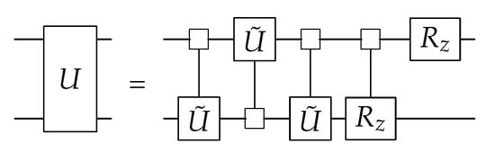
Figure 9.
Recursive CSD decomposition [21].
5.7. Quantum Shannon Decomposition
In [22], another way of using the CSD from Section 5.6, called Quantum Shannon Decomposition (QSD), is introduced. The decomposition of a two-qubit gate is shown in Figure 10.
Figure 10.
Quantum Shannon Decomposition [22].
The start of the decomposition is the same as in Section 5.6, but the L and R matrices are decomposed using eigenvalue decomposition. This is shown in Figure 11. The resulting matrices are unitary gates applied to one less qubit than the starting unitary. This leads to the circuit in Figure 10, where the D-matrix is implemented as a multi-controlled gate.
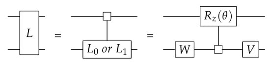
Figure 11.
Decomposition of the L matrix in QSD [22].
Quantum Shannon Decomposition is applied recursively until the final one-qubit gates can be implemented with ZYZ decomposition. This means that only the multi-controlled rotation gates contribute to the number of CNOTs, each of which requires CNOT gates for a single step of the recursion of an n-qubit gate. This leads to a total CNOT count of for this decomposition method.
There are two optimizations that can be implemented on top of this implementation of Quantum Shannon Decomposition. The first is to stop the recursion at two-qubit gates and translate those as in Section 5.4. The second optimization is to implement the central multi-controlled gate using CZ gates rather than CNOTs, of which one can be absorbed into the neighboring multiplexer. This results in one fewer CNOT gate at each level of the recursion. With these two implementations, the CNOT count comes to [22] .
5.8. Selection of the Algorithm
For each decomposition method, the CNOT gate counts are compiled in Table 1 and plotted in Figure 12. As an indication, the number of CNOT gates resulting from the decomposition of a one to five-qubit unitary gate is given, along with the general formulas for the number of CNOT gates resulting from the decomposition of an n-qubit gate, if such a formula were available.

Table 1.
CNOT counts for different implementations of unitary decomposition for one through five-qubit gates, as well as an n-qubit unitary gate.
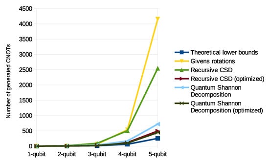
Figure 12.
CNOT counts for different implementations of unitary decomposition for one through five-qubit gates. The chosen algorithm is shown in bold.
As can be seen in Table 1, the optimized version of QSD results in the fewest CNOT gates. The choice was therefore made to implement this decomposition, although not the optimized version. The optimizations from [16] can be implemented without any modifications to a base implementation of the algorithm.
Besides that, QSD has several other advantages. The recursion is performed at general n-qubit gates rather than multi-controlled one-qubit gates, which makes it relatively simple to implement. If algorithmic implementations for three-qubit, four-qubit or five-qubit or bigger general gates are found, they can be easily implemented. The same goes for other specific optimizations. In addition, because the mathematical decompositions are done separately for each step in the recursion, rather than all at once at the beginning, any underlying structure in the beginning or intermediate matrices can be taken advantage of immediately, therefore potentially skipping many computational steps as well as decreasing the size of the resulting circuit.
For these reasons, the choice was made to go with Quantum Shannon Decomposition for the implementation of unitary decomposition in OpenQL.
6. Implementation
The implementation of the decomposition in OpenQL is split into two parts: the calculation of all of the rotation angles, and the generation of the circuit. This is done so that the implementation is independent from OpenQL.
An example of unitary decomposition in OpenQL can be found in Code Listing 1.
For unitary decomposition in OpenQl, first a Unitary object is defined, which is then decomposed to calculate all the angles for all the rotation gates. The Unitary is then added to a kernel as any other gate. The kernel is added to a program, which is compiled with a compiler. The implementation is thus split between the Unitary class and the call to kernel.gate().
Listing 1. Using unitary decomposition in OpenQL.
| import os |
| from openql import openql as ql |
| import numpy as np |
| import sys |
| nqubits = int(sys.argv[1]) |
| ql.set_option(’output_dir’, os.path.join(curdir, ’output’)) |
| ql.set_option(’log_level’, ’LOG_ERROR’); |
| platf = ql.Platform("starmon", os.path.join(curdir, ’config.json’)) |
| program = ql.Program(’example’, platf, nqubits) |
| kernel = ql.Kernel("newKernel") |
| compiler = ql.Compiler(’compiler1’) |
| matrix = np.load(’data/out_’ + str(nqubits) + ".npy") |
| u1 = ql.Unitary("testname",matrix) |
| u1.decompose() |
| kernel.gate(u1, range(0,nqubits)) |
| program.add_kernel(kernel) |
| compiler.compile(program) |
6.1. The Unitary Class
The Unitary is instantiated with a string and an array. The content of this array is the unitary matrix, which is of size for an n-qubit gate. The complete Quantum Shannon Decomposition is computed only when “decompose()” is called, and the calculated angles for the resulting rotation gates are added to a list. This is done so that the Unitary can be used multiple times in a program without the recalculation of the whole decomposition.
However, before the decomposition is started, it is first checked whether the input matrix is unitary. If this is the case, all of the intermediate matrices will also be unitary [19], so this check is only necessary once. Furthermore, all of the Gray code matrices needed for the multi-controlled rotation gates are added to a lookup table so they do not need to be calculated anew at each decomposition step.
To make certain that the decomposition is correct, each single intermediate decomposition is checked. For each step, only three matrices need to be multiplied, and this saves any calculations that might be performed on an incorrect matrix. If any step of the decomposition is not correct, an exception is thrown and the decomposition is stopped.
The Eigen [23] library is used to perform singular value decomposition (SVD), eigenvalue decomposition and matrix multiplication. The recursion is centered on a main function, which takes as parameters a unitary matrix and the number of qubits. The latter is to keep track of the level of recursion.
Computation of the CSD is done using the method from [19], which uses SVD. The demultiplexing function uses Schur matrix decomposition for (sub)matrices smaller than and eigenvalue decomposition for bigger matrices. This is done because Schur matrix decomposition is faster for small matrices [23].
The algorithm is recursive, and the demultiplexing step calls on the main function again for the decomposition of the smaller unitary matrices. If the matrices are of size , the rotation angles for the one-qubit rotation gates are calculated using ZYZ decomposition as in Section 5.3.
Because the Unitary does not have access to the qubit numbers of the circuit, only the angles for the multi-controlled and are calculated at this point. This is done as in Section 3.6 by solving the following matrix equalities:
where is a square matrix where all the entries are either “+1” or “−1”, which are calculated using Gray code using Equation (20).
where the exponent is the bit-wise inner product of two binary vectors: and . is the integer i, and is the jth value of the Gray code.
For the multi-controlled gate, the values of are calculated by taking the arc sine of the diagonal entries of the S-matrix from the CSD.
For the multi-controlled gates, the values of is calculated by taking the natural logarithm of the D-matrix from the demultiplexing.
All the angles for all rotation gates are added to a list, which is used to generate the correct gates when the Unitary is added to a circuit.
6.2. Circuit Assembly
At the kernel level, when the (decomposed) Unitary object is added to the circuit, the gates and CNOTs are assembled and added to the circuit list. At this point, it is checked whether the Unitary is decomposed and if it is applied to the correct number of qubits. The first is checked from a flag that is set to “true” at the end of the decomposition. The latter is calculated from the size of the unitary matrix, which should be for an n-qubit gate.
Because the kernel only has the qubit numbers and the list of rotation angles, it does not have insight into whether any optimizations have happened. Therefore, the gates are added purely sequentially to the circuit, and each recursive call to the main function returns the total number of rotation angles used up until that point. If gates have been removed by an optimization, a specific angle is added to the circuit which signals how many gates have been removed, and these gates are skipped during circuit generation.
It is expected that the decomposition will take the most time to compute, as well as the most memory, since it contains the mathematical algorithms and matrix multiplications. Comparatively, using the calculated angles to make the circuit will not require much time or memory. Thus, adding the circuit sequentially is not expected to have much of an impact on the total resources required by the circuit, while it allows for a much more modular implementation of unitary decomposition.
6.3. Compilation of the OpenQL Program
After all gates have been added to the circuit, the kernel is added to a program which is compiled in OpenQL. From this point, the gates from the decomposition are handled in the same way as any manually added gates. Thus, the features and optimizations from the lower levels of the programming language can be fully used for the circuit [5]. Afterwards, the circuit is transformed into quantum assembly language and written to an output file as usual, or directly passed on to the simulator.
7. Implementation Optimization
For the execution of the resulting circuit, it is important that it is as short as possible for the reasons mentioned in Section 5. To this end, the algorithm itself was selected to generate as few gates as possible. Combining and removing individual gates is performed in a later compile step by the OpenQL compiler [5], but more structural optimizations can be performed during the decomposition. For example, QAM, one of the algorithms from Section 2, generates a unitary matrix that has an internal structure that can be used to skip many steps in the recursion (see Section 2). The implemented optimizations take advantage of the matrix structure through the early detection of multiplexers and the detection of unaffected qubits.
7.1. Detection of Multiplexers
Before the CSD is started, it is checked whether the upper right and lower left quarters of the matrix are already zero-matrices. If that is the case, the matrix already has the structure of a multiplexer and is directly passed to the demultiplexing step. This is signaled to the kernel by adding a specific gate angle to the list of rotation angles. This operation halves the number of resulting gates for this step of the decomposition.
7.2. Unaffected Qubits
If a decomposition step leaves a qubit unaffected, then it is not necessary to apply any gates to that qubit, and an n-qubit gate can be handled as an -qubit gate. This reduces the resulting number of gates for this step by more than . Thus, before the main decomposition is called, it is checked if the matrix is of the form or . Each step of the QSD evaluates unitary gates on one less qubit, so any unaffected qubits become the first or last qubit at some point in the decomposition. If an unaffected qubit is detected, this is also signaled to the kernel. The unitary matrix of size is then assembled and passed back to the main function of the decomposition.
7.3. Execution Time Optimizations
There are also some optimizations to reduce the execution time and memory use of the decomposition.
One of the things done to reduce the total execution time and memory use is the fitting of “.noalias()” flags to all places where the product of multiple matrices is assigned to a different matrix. The Eigen library assumes aliasing for all such operations, and without this flag it evaluates the result of a matrix product into a temporary matrix that is then copied [23]. Another optimization is that all matrices are passed as references where possible to prevent any unnecessary copying of data.
The execution time and memory use of the decomposition after these and other optimizations can be found in Section 8. Circuit generation and its associated steps scale with approximately , which is as expected since that implies a linear relation with the number of matrix elements and the length of the circuit. The decomposition itself scales as [24].
8. Results
The execution time of different parts of the decomposition is measured as the elapsed wall-clock time, with measurements in between function calls to determine the relative time consumption. The final execution times are shown in Figure 13. These tests were executed using a Dell Latitude 7400 with an 8th Generation Intel® Core™ i7-8665U Processor and 2× 4GiB DDR4 RAM.
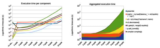
Figure 13.
Execution time for the timed intervals, for different sizes of unitary matrices.
The program in Code Listing has been used to determine the execution time and memory used by the decomposition. Unitary matrices of sizes to were randomly generated first, using QiBAM as outlined in Section 2. The matrices were stored as binary files and loaded as required for the decompositions. The decomposition was repeated 1000 times for the smaller gates and 100 times for the decomposition of the 10-qubit gate in OpenQL, with varying numbers for the intermediate sizes. The execution time and memory use as reported in this paper are the averages of these runs.
To measure execution time, the Python “time” package was used to determine the time difference between the start and various points of the program. The time for each part of the code, as well as the resulting aggregated execution time, can be found in Figure 13 and Table 2.
Table 2.
Total execution time at each line of Listing 1 for the decomposition of matrices of different sizes, in seconds.
As expected, the decomposition itself took the most time—more than 10 times that of any other part. This is because of the considerable mathematical decompositions and the number of matrix operations. One of the algorithms used in the decomposition is eigenvalue decomposition, which is an iterative algorithm that requires operations for an matrix [25]. The data also show that the generation of the rotation gates and CNOTs does not contribute much to the total execution time of the algorithm, as expected. In addition, since the complete decomposition is calculated at design time, it does not influence the run-time of the final circuit when it is executed on a quantum accelerator.
The same program has also been used to determine the memory allocation. This has been measured using the Python memory_profiler package. The results of this are shown in Table 3 and Figure 14. After an initial allocation of about 40 MiB, noteworthy additional allocation of memory occurs only when k.gate(...) is called. This means that the complete unitary decomposition requires much less memory than generating and storing the resulting circuit in OpenQL.
Table 3.
Additional memory allocated at each line of Listing 1 for the decomposition of unitary matrices of different sizes, in MiB.
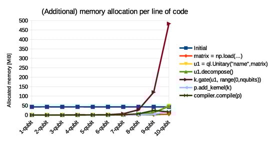
Figure 14.
Additional memory allocated per line, for different sizes of unitary matrices.
9. Other Implementations
We compare our OpenQL implementation to Qubiter and UniversalQCompiler. These two are the only other quantum programming languages that, at the time of writing, also offer unitary decomposition.
9.1. Qubiter
Qubiter [18] is a quantum compiler/programming language that aims to provide a set of tools for designing and simulating quantum circuits. As part of that, they offer unitary decomposition based on the recursive CSD from Section 5.6. Qubiter is written in Python and uses numpy for the mathematics, as well as the LAPACK cuncsd function for the CSD [20].
9.2. UniversalQCompiler
UniversalQCompiler (UQC) is a software package written in the Mathematica language that can be used to decompose various quantum operations into CNOT gates and single qubit rotation gates. The resulting circuits can be displayed graphically or translated to OpenQASM, a quantum assembly language used by IBMQ, among others [26].
One of the types of decomposition they have implemented is unitary decomposition using QSD from [27]. This method produces CNOTs, which is the same number as in [22].
10. Comparison to Other Implementations
We compare the execution time and the number of gates our implementation generates against Qubiter and UQC.
To obtain the total gate count, we use the number of lines in the output quantum assembly, which also includes rotation gates and not just CNOTs. The results for OpenQL, Qubiter and UQC are plotted in Figure 15. All of the implementations use an exact decomposition algorithm and therefore generate a constant number of gates for each size of the (non-sparse) input matrix.
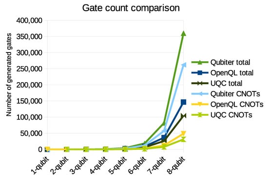
Figure 15.
Number of generated CNOTs and total gates for OpenQL, UQC and Qubiter from the decomposition of different sizes of unitary matrices.
It is clear that OpenQL always generates fewer gates than Qubiter, and almost all of the difference is in the number of CNOTs. This is because we use QSD in our implementation of unitary decomposition in OpenQL. For a 10-qubit gate, unitary decomposition with OpenQL generates half as many CNOTs as Qubiter, and produces a total circuit that is almost 3 times as short.
When compared to UQC, our OpenQL implementation generates about 50% more of any type of gate. This difference is because UQC uses an optimal circuit at the two-qubit gate level, where OpenQL uses another iteration of QSD and then ZYZ-decomposition, which results in more gates.
The implementations are also compared on the time used to compute the unitary decompositions. The total wall-clock execution time for the decomposition and circuit generation of 2 to 10-qubit unitary gates can be found in Figure 16. The total execution time of all decompositions scales approximately linearly with the input matrix size ( for an n-qubit gate) for the decomposition of small matrices due to matrix loading and circuit generation operations and then becomes when the decomposition of bigger matrices begins to take more time than the other steps. This is around the decomposition of seven-qubit unitary gates.
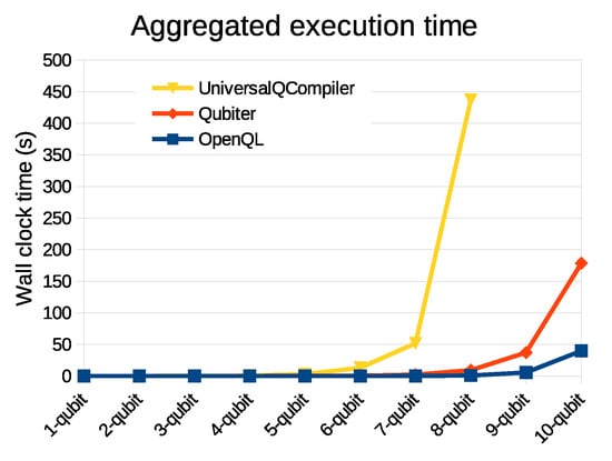
Figure 16.
Execution time of the decomposition and circuit generation for OpenQL, Qubiter and UQC for different sizes of unitary matrices.
As can be seen in the figure, OpenQL is considerably faster than Qubiter and UQC. When comparing the total execution times, it becomes clear that the OpenQL implementation takes more time per input matrix element () due to the use of CSD. Qubiter does not have that issue, but using unitary decomposition in OpenQL is about 10 to 100 times faster for the decomposition of 1 to 10-qubit unitary gates. This can most likely be attributed to the languages the compilers are programmed in and how well the implementation takes advantage of the programming language. Qubiter is written in Python and the UQC is written in Mathematica, both of which are considerably slower than C++, used for OpenQL [28].
In addition to being faster, unitary decomposition in OpenQL generates a much shorter circuit for all sizes of unitary matrices compared to Qubiter. For UQC, the tests were stopped at the decomposition of an eight-qubit unitary gate, which took approximately 450 s. Decomposing a nine-qubit gate was stopped after an hour, when it had still not produced results. As a result, although the decomposition in UQC does result in fewer gates, it also takes about 500 times as long as decomposition in OpenQL.
11. Conclusions and Future Work
With the implementation of unitary decomposition, OpenQL can now be used for any quantum algorithm that uses arbitrary unitary gates. One such algorithm is QiBAM [8], which cannot be implemented without unitary decomposition.
The decomposition generates more gates than the theoretical minimum, but the structure of the decomposition means that further optimizations can be easily integrated with the current implementation. The decomposition is performed using Quantum Shannon Decomposition, which is up to 10 times more efficient in the number of generated gates than Qubiter and only 50% less efficient than the implementation of UQC. Two optimizations were implemented to take advantage of the internal structure of the input or intermediate unitary matrices, which can drastically reduce the length of the resulting circuit. With these optimizations, the final resulting gate count can be much lower than the illustrated worst case numbers.
The decomposition results in CNOT gates and total gates. Although the execution time of the decomposition is for matrices of size , for the decomposition of up to 10-qubit gates, our implementation is 10–100 times faster than Qubiter and about 500 times faster than the implementation in UQC.
There are several avenues that can further bring down the number of gates the decomposition generates, which are as follows:
- The implementation of a minimum two-qubit circuit, such as the one described in [22] using the method from [29], if applicable;
- Additionally, the implementation of a universal three-qubit gate, such as the one in [30];
- Implementing the multiplexed gate with a CZ gate, as expressed in [22];
- Reworking the QSD so that the intermediate matrices cancel out, as the input matrix has fewer degrees of freedom than the matrices resulting from the QSD. Therefore, it might be possible to choose some of these intermediate matrices in such a way that they can be decomposed using fewer elementary gates;
- The implementation of other specific efficient decompositions, such as controlled unitary gates (as opposed to uniformly controlled gates), quantum multiplexers or specialized multi-controlled rotation gates.
Author Contributions
Methodology, A.M.K. and A.S.; software, A.M.K. and I.A.; supervision, Z.A.-A. and K.B.; writing—original draft, A.M.K.; writing—review and editing, Z.A.-A. All authors have read and agreed to the published version of the manuscript.
Funding
This research received no external funding.
Institutional Review Board Statement
Not applicable.
Informed Consent Statement
Not applicable.
Data Availability Statement
The OpenQL source code, including the implementation of unitary decomposition presented in this paper, is available at https://github.com/QE-Lab/OpenQL (accessed on 6 January 2022).
Conflicts of Interest
The authors declare no conflict of interest.
References
- Shor, P.W. Polynomial-Time Algorithms for Prime Factorization and Discrete Logarithms on a Quantum Computer. SIAM J. Comput. 1997, 26, 1484–1509. [Google Scholar] [CrossRef] [Green Version]
- Grover, L.K. Quantum mechanics helps in searching for a needle in a haystack. Phys. Rev. Lett. 1997, 79, 325–328. [Google Scholar]
- Almudever, C.G.; Lao, L.; Wille, R.; Guerreschi, G.G. Realizing Quantum Algorithms on Real Quantum Computing Devices. In Proceedings of the 2020 Design, Automation Test in Europe Conference Exhibition (DATE), Grenoble, France, 9–13 March 2020; pp. 864–872. [Google Scholar]
- Tannu, S.S.; Qureshi, M.K. Not All Qubits Are Created Equal: A Case for Variability-Aware Policies for NISQ-Era Quantum Computers. In Proceedings of the ASPLOS ’19: Twenty-Fourth International Conference on Architectural Support for Programming Languages and Operating Systems, Providence, RI, USA, 13–17 April 2019; Association for Computing Machinery: New York, NY, USA, 2019; pp. 987–999. [Google Scholar]
- Khammassi, N.; Ashraf, I.; Someren, J.V.; Nane, R.; Krol, A.M.; Rol, M.A.; Lao, L.; Bertels, K.; Almudever, C.G. OpenQL: A Portable Quantum Programming Framework for Quantum Accelerators. ACM J. Emerg. Technol. Comput. Syst. 2022, 18, 1–24. [Google Scholar]
- Allen, G.D. Unitary Matrices. In Lectures on Linear Algebra and Matrices; Texas A&M University: College Station, TX, USA, 2003; Chapter 4; pp. 157–180. [Google Scholar]
- Houtgast, E.J.; Sima, V.M.; Bertels, K.; Al-Ars, Z. Hardware acceleration of BWA-MEM genomic short read mapping for longer read lengths. Comput. Biol. Chem. 2018, 75, 54–64. [Google Scholar] [CrossRef] [PubMed]
- Sarkar, A.; Al-Ars, Z.; Almudever, C.G.; Bertels, K.L.M. QiBAM: Approximate Sub-String Index Search on Quantum Accelerators Applied to DNA Read Alignment. Electronics 2021, 10, 2433. [Google Scholar] [CrossRef]
- Ventura, D.; Martinez, T. Quantum associative memory. Inf. Sci. 2000, 124, 273–296. [Google Scholar] [CrossRef] [Green Version]
- Deutsch, D.E.; Penrose, R. Quantum computational networks. Proc. R. Soc. Lond. A Math. Phys. Sci. 1989, 425, 73–90. [Google Scholar] [CrossRef]
- Savage, A. Introduction to Lie Groups. In Course Notes of MAT 1411/MAT 5158; University of Ottawa: Ottawa, ON, Canada, 2015. [Google Scholar]
- Bullock, S.S.; Markov, I.L. Arbitrary two-qubit computation in 23 elementary gates. Phys. Rev. A 2003, 68, 012318. [Google Scholar] [CrossRef] [Green Version]
- Möttönen, M.; Vartiainen, J.J.; Bergholm, V.; Salomaa, M.M. Quantum Circuits for General Multiqubit Gates. Phys. Rev. Lett. 2004, 93, 130502. [Google Scholar]
- Mooney, G.J.; Hill, C.D.; Hollenberg, L.C.L. Entanglement in a 20-Qubit Superconducting Quantum Computer. Sci. Rep. 2019, 9, 1–8. [Google Scholar] [CrossRef] [Green Version]
- Shende, V.V.; Markov, I.L.; Bullock, S.S. Minimal universal two-qubit controlled-NOT-based circuits. Phys. Rev. A 2004, 69, 062321. [Google Scholar] [CrossRef] [Green Version]
- Vartiainen, J.; Möttönen, M.; Salomaa, M. Efficient Decomposition of Quantum Gates. Phys. Rev. Lett. 2004, 92, 177902. [Google Scholar]
- Barenco, A.; Bennett, C.H.; Cleve, R.; DiVincenzo, D.P.; Margolus, N.; Shor, P.; Sleator, T.; Smolin, J.; Weinfurter, H. Elementary gates for quantum computation. Phys. Rev. A 1995, 52, 3457. [Google Scholar] [PubMed] [Green Version]
- Tucci, R.R. A Rudimentary Quantum Compiler. arXiv 1999, arXiv:9902062. [Google Scholar]
- Paige, C.; Wei, M. History and generality of the CS decomposition. Linear Algebra Its Appl. 1994, 208, 303–326. [Google Scholar] [CrossRef] [Green Version]
- Dekant, H.; Tregillus, H.; Tucci, R.; Yin, T. Qubiter at GitHub. 2020. Available online: github.com/artiste-qb-net/qubiter (accessed on 6 January 2022).
- Möttönen, M.; Vartiainen, J. Trends in Quantum Computing Research; Decompositions of General Quantum Gates; Nova Science Publishers, Inc.: Hauppauge, NY, USA, 2006; pp. 149–170. [Google Scholar]
- Shende, V.; Bullock, S.; Markov, I. Synthesis of Quantum Logic Circuits. Comput.-Aided Des. Integr. Circuits Syst. IEEE Trans. 2006, 25, 1000–1010. [Google Scholar] [CrossRef] [Green Version]
- Guennebaud, G.; Jacob, B. The Eigen Documentation v3. 2019. Available online: http://eigen.tuxfamily.org (accessed on 20 July 2020).
- Sutton, B.D. Computing the complete CS decomposition. Numer. Algor. 2009, 50, 33–65. [Google Scholar] [CrossRef] [Green Version]
- Blackford, S.; Moore, R.; Drakos, N. LAPACK Users’ Guide. Available online: https://www.netlib.org/lapack/lug/ (accessed on 23 October 2020).
- Iten, R.; Reardon-Smith, O.; Malvetti, E.; Mondada, L.; Pauvert, G.; Redmond, E.; Kohli, R.S.; Colbeck, R. Introduction to UniversalQCompiler. arXiv 2021, arXiv:1904.01072. [Google Scholar]
- Iten, R.; Colbeck, R.; Kukuljan, I.; Home, J.; Christandl, M. Quantum circuits for isometries. Phys. Rev. A 2016, 93, 032318. [Google Scholar] [CrossRef] [Green Version]
- Aruoba, S.B.; Fernández-Villaverde, J. A comparison of programming languages in macroeconomics. J. Econ. Dyn. Control 2015, 58, 265–273. [Google Scholar] [CrossRef] [Green Version]
- de Guise, H.; Di Matteo, O.; Sánchez-Soto, L.L. Simple factorization of unitary transformations. Phys. Rev. A 2018, 97, 022328. [Google Scholar] [CrossRef]
- Vatan, F.; Williams, C.P. Realization of a General Three-Qubit Quantum Gate. arXiv 2004, arXiv:0401178. [Google Scholar]
Publisher’s Note: MDPI stays neutral with regard to jurisdictional claims in published maps and institutional affiliations. |
© 2022 by the authors. Licensee MDPI, Basel, Switzerland. This article is an open access article distributed under the terms and conditions of the Creative Commons Attribution (CC BY) license (https://creativecommons.org/licenses/by/4.0/).