Numerical Study of Rock Damage Mechanism Induced by Blasting Excavation Using Finite Discrete Element Method

Abstract

In this paper, the mechanism of rock damage induced by blasting excavation is numerically studied by using an FDEM-based multiphysics fracture analysis software, MultiFracS. Based on the drainage channel project of Guanggu 1st Road to Gaoxin 4th Road, a numerical model considering the near-field fracture process is established to study the influence of a millisecond delay and construction technology on the blasting excavation. Firstly, the double side drift method model is established to analyze the influence of different millisecond delays on the peak blasting vibration velocity. Then, the rock fracture process of the surrounding rock around the blast holes under the blasting excavation construction technology of the double side drift method, the reserved core soil method, and the CRD method is studied, respectively. The numerical simulation results show that the mainshock phases of the blasting vibration velocity waveform generated by different bores overlap when the millisecond delay is small. With the increase in the millisecond delay, the mainshock phase is gradually separated, and the superposition effect of the blasting vibration is weakened. When the millisecond delay is greater than 40 ms, the peak blasting vibration velocity is not affected by the millisecond delay. In the three kinds of blasting excavation construction technologies, the double side drift method has a better effect on the deformation and the fracture control of the surrounding rock. The optimal millisecond delay and the rock fracture evolution process of the surrounding rock around blast holes with different blasting excavation construction technologies are obtained.

1. Introduction

In underground engineering, such as tunnel excavation and mining engineering, blasting is an effective measure to break up rock mass. Although the application of blasting significantly improves the efficiency of underground cavern excavation, it causes damage to the surrounding rock. To reduce the damage of blasting to the surrounding rock, the blasting excavation design and construction technology need to be optimized.

Therefore, the rock fracture process caused by blasting is characterized and classified. Ramulu et al. [1] established a damage model of compact basalt and almond-shaped basalt to study the damage of dynamic load on basalt rock mass. Kim et al. [2] established a split-Hopkinson pressure bar (SHPB) model to study the stress–strain relationship of rocks under dynamic loads, and a series of parameters affecting the dynamic mechanical properties of rocks were obtained. Singh et al. [3] conducted field blasting tests by controlling blast hole spacings and charging methods and studied the design modes and blasting excavation construction technologies. Villaescusa et al. [4] used a triaxial blasting vibration waveform monitoring device to monitor the rock mass damage in the mining field and established a rock damage model for blasting design.

However, the blasting excavation test has the disadvantages of a high safety risk, complicated operation, poor repeatability, and high cost. Recently, more and more scholars are using numerical simulation to study blasting excavation. Tao et al. [5] used a three-dimensional numerical simulation to study the fracturing effect of the surrounding rock under the excavation stress. Liu et al. [6] studied the expansion process of the rock fracture propagation process during blasting excavation in the TASQ tunnel of the Aspo laboratory. Saiang et al. [7] used a finite-difference program (FLAC) to study the mechanical behavior of blast-damaged rock masses in shallow tunnels, and the results showed that the blast damage area can significantly induce boundary stress and affect the distribution and magnitude of ground deformation. Li et al. [8] proposed a mathematical model for the dynamic excavation response of a circular roadway under hydrostatic pressure and analyzed the dynamic response mechanism of the surrounding rock under different unloading rates and different unloading paths using PFC. Yang et al. [9] used the LS-DYNA to simulate the rock damage evolution process under the dynamic stress redistribution and explosive loading and confirmed that the dynamic stress redistribution generates additional stress fluctuations, resulting in a larger rock damage area. Xie et al. [10] introduced a new damage model in the LS-DYNA to study the effect of in situ stress distribution on the development of damage zones around deep-buried tunnels during the cutting blasting process. However, the above research rarely considers the near-field fracture evolution of the tunnel surrounding rock.

The finite-discrete element method (FDEM) proposed by Munjiza [11,12] has been successfully used to model the transition from continuum to discontinuity and developed the open-source program Y2D. The FDEM absorbs the advantages of the explicit finite element method for solving deformation and stress, the advantages of the discrete element method for dealing with contact, and the advantages of the cohesive element model for simulating fracture. In the FDEM, the solution domain is divided into solid finite element meshes, and initial zero thickness joint elements that are similar to cohesion elements are inserted into the boundaries of the solid elements. In addition, the initiation and propagation of cracks are simulated by the fracture of joint elements. The deformation and stress of the continuum are characterized by the deformation of the solid elements and the bonding effect of the unbroken joint elements. Secondly, the NBS contact detection algorithm and potential contact force are used to deal with the contact problems caused by crack closure, sliding, and block collision.

In recent years, the FDEM has been widely used in tunnel excavation [13,14], laboratory test-scale simulation [15,16], etc. For example, Rougier et al. [17] used a 3D-FDEM to perform a full-scale three-dimensional analysis of the SHPB test for granite materials. The softening behavior of the sample after crushing can be reproduced, and the simulation results are consistent with the laboratory observations. Fukuda et al. [18] combined the FDEM and GPU parallel technology to simulate a full-scale SHPB test and observed the dynamic fracturing process and stress response phenomena of a Brazilian disk marble specimen. Hamdi et al. [19] used the FDEM to simulate the complete 3D fracture process in routine laboratory tests, including Brazilian splitting and uniaxial and biaxial compression tests. The numerical results are in good agreement with the experiments, which shows that the FDEM can simulate the rock fracture well.

Later, Yan [20] proposed a new potential function, which not only retained all the characteristics of the original potential function in the FDEM but also reduced the dependence on the mesh. Yan developed a series of 2D/3D hydro-mechanical coupling models [21,22,23,24,25,26,27,28], contact heat transfer models [29,30,31], thermo-mechanical coupling models [32,33,34,35,36], hydro-thermal coupling models [37], and moisture diffusion-fracture coupling models [38,39,40], which make it possible to solve complex problems such as hydraulic fracturing, thermal cracking, shrinkage cracking, etc. Later, these models were integrated and combined with GPU parallel technology to develop the MultiFracS software by Yan [36]. From the above discussion, it can be seen that the FDEM has been used in various fields [41], and its related functional modules have been continuously improved. The functions of the FDEM have completed the transition from pure mechanical fracture calculation to multi-physics fracture calculation, and from small-scale 2D fracture calculation to larger-scale 3D fracture calculation.

In view of the unique advantages of the FDEM, we use the FDEM-based software MultiFracS to establish a numerical model for tunnel blasting excavation, considering near-field fracture and breakage. This model is used to study the effects of a millisecond delay and different blasting excavation construction technologies, including the blasting vibration velocity and the degree of fracture of the surrounding rock around the blast hole.

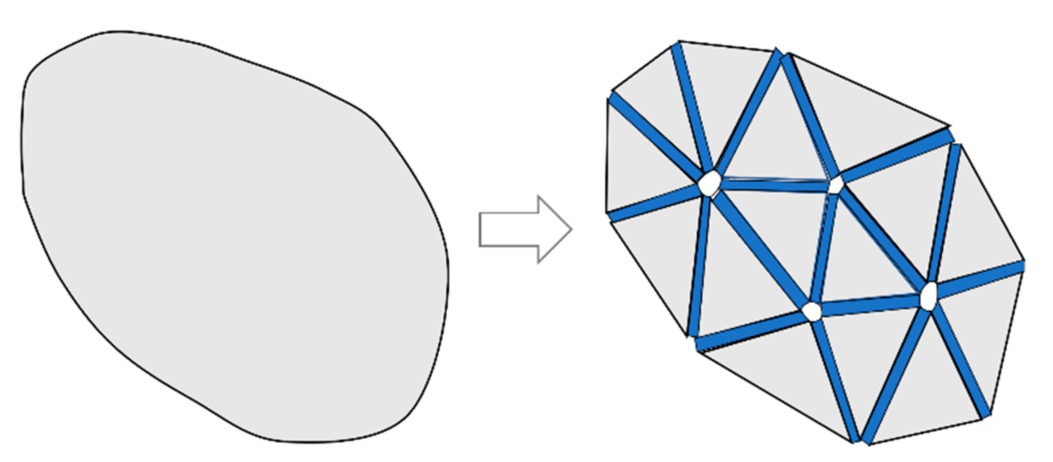
2. Fundamental of FDEM

2.1. Basic Equation

The FDEM combines the advantages of the finite element method and discrete element method. In the FDEM, the explicit finite element method is used to calculate the stress and strain of the element, the discrete element method is used for contact detection and contact force, and the joint element is used to simulate the initiation and propagation of cracks. The entire solution domain is discretized into a series of triangular elements. The relevant information (mass, load) and motion information (displacement, velocity, acceleration) of each triangular element are equivalent to the nodes of the triangular element, as shown in Figure 1. Therefore, the motion law of the entire solution domain can be determined through the motion law of these triangular element nodes. The velocity and displacement of any point in the triangular element can be obtained by linear interpolation of the three nodes constituting the triangular element. According to Newton’s second law, the position and velocity of these nodes of the element at any time can be determined when the mass of each node and the total node force are determined. The equation of motion of the node is as follows [20]:

$$M\frac{{\partial }^{2}x}{\partial t^2}+C\frac{\partial x}{\partial t}=F$$

(1)

where the M is the nodal mass, $C$ is the damping coefficient, and $F$ is the total nodal force, which is equal to the vector sum of the nodal forces caused by the contact force, the deformation of the triangular element, the deformation of the joint element, and other external loads such as gravity.

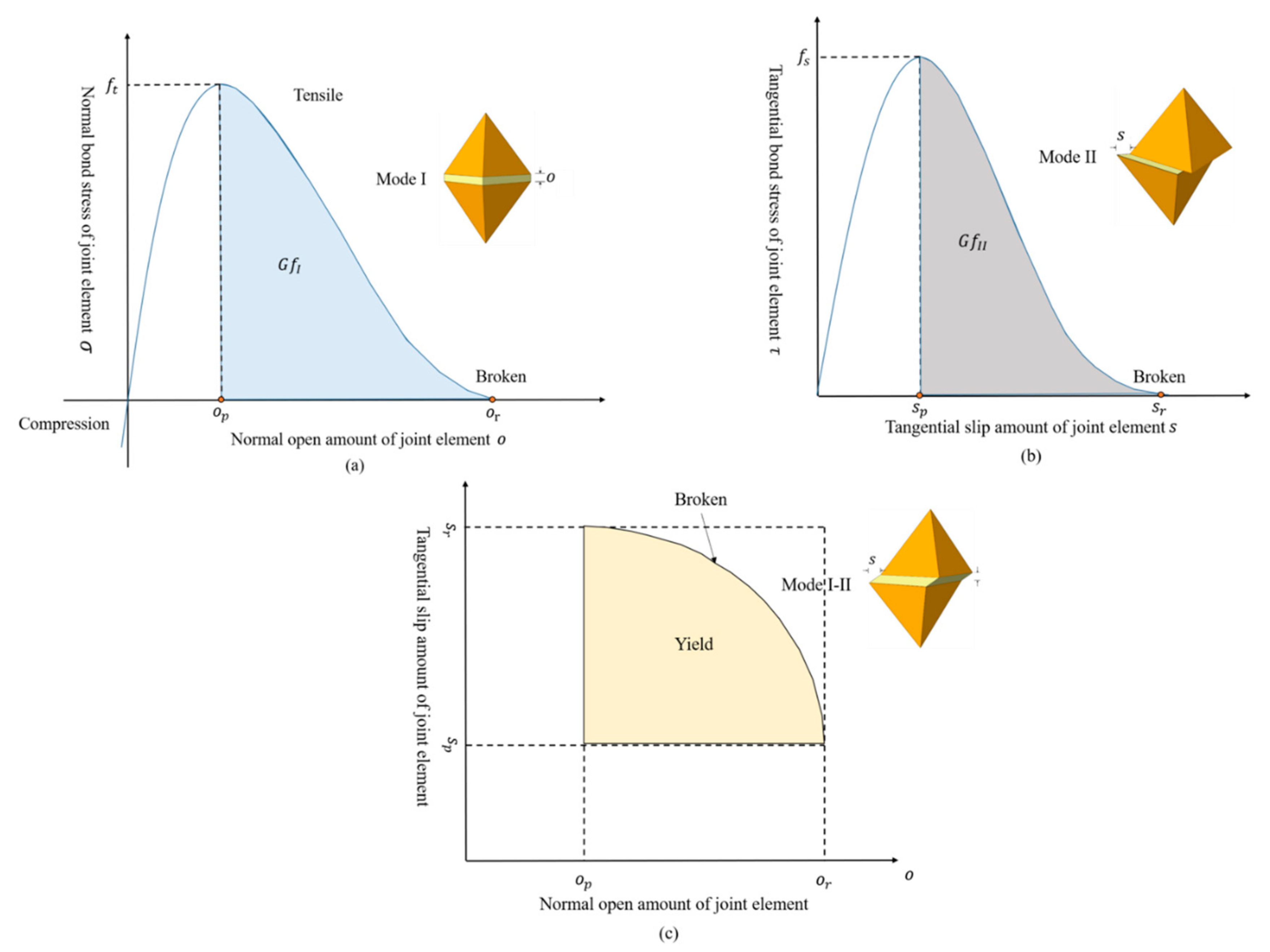
2.2. Fracture Constitutive Model for the Joint Element

In the FDEM, the initiation and propagation of cracks are controlled by the constitutive fracture model of the joint element. The four nodes of the joint element are shared with the two adjacent triangular elements on both sides. Therefore, the initiation and propagation of cracks are only along the boundary of the triangular element. According to the relative displacement state of the nodes of the joint element and the fracture constitutive model, it can be judged whether the joint element is yielded, the I-type tension failure, II-type shear failure, or I-II mixed tension–shear failure [20].

The relationship between the normal and tangential traction force and the normal opening and tangential slip is shown in Equations (2) and (3). These two equations mainly represent the softening behavior in the latter part of the tensile and shear peaks, as shown in Figure 2.

$$\sigma =\left\{\begin{array}{l}\begin{array}{cc}{p}_{f}o,& o<0\end{array}\hfill \\ \begin{array}{cc}f(D)T_s,& o\ge 0\end{array}\hfill \end{array}\right.$$

(2)

where P_f is the penalty parameter of the joint element, o is the normal opening, T_s is the tensile strength.

$$\tau =\left\{\begin{array}{l}\begin{array}{cc}(c-\sigma \tan \varphi )f(D),& \sigma <0\end{array}\hfill \\ \begin{array}{cc}cf(D),& \sigma \ge 0\end{array}\hfill \end{array}\right.$$

(3)

where D is the damage variable of the joint element, which can be specifically calculated.

When the joint element is in an elastic state:

$$\begin{array}{cc}D=0,& o\le o_p \mathrm{and} \left|s\right|=0\end{array}$$

(4)

when the joint element is in a pure tension state:

$$\begin{array}{cc}D=\frac{o-o_p}{o_t-o_p},& o>o_p \mathrm{and} \left|s\right|=0\end{array}$$

(5)

where $o_p$ is the corresponding normal opening amount when the joint element is at the peak tensile stress (equal to the tensile strength), $o_t$ is the critical opening amount when the joint element is tensile-fractured. When the opening amount of the joint element reaches the critical opening amount $o_t$, the damage variable D is 1. At this moment, the tensile stress is reduced to 0 and a tensile crack occurs. $o_t$ can be calculated according to the fracture energy of Mode I according to the following formula:

$$G_{fI}={\displaystyle {\int }_0^{o_t}\sigma (o)do}$$

(6)

For pure shear state:

$$\begin{array}{cc}D=\frac{\left|s\right|-s_p}{s_t-s_p},& \left|s\right|>s_p \mathrm{and} o\le 0\end{array}$$

(7)

where $s_p$ is the corresponding tangential slip when the joint element is at the peak shear stress (equal to the shear strength), and $s_t$ is the critical tangential slip when the joint element is tensile-fractured. When the tangential slip reaches the critical slip $s_t$, the damage variable D is 1. At this moment, the tangential shear stress is reduced to 0 and a shear crack occurs. $s_t$ can be calculated according to the fracture energy of Mode II by:

$$G_{fII}={\displaystyle {\int }_0^{s_t}\tau (s)ds}$$

(8)

For the mixed tensile–shear state:

$$\begin{array}{c}D=\sqrt{{\left(\frac{o-o_p}{o_t-o_p}\right)}^2+{\left(\frac{\left|s\right|-s_p}{s_t-s_p}\right)}^2},\end{array}o>o_p \mathrm{or} \left|s\right|>s_p$$

(9)

According to Equations (4), (5), (7), and (9), the damage degree of the joint element can be calculated. If the damage variable D is greater than 1, set D to1. At this time, the joint element breaks, and a crack occurs.

Figure 2. Fracture constitutive model of joint elements: (a) tensile failure; (b) shear failure; (c) mixed tensile and shear failure [11,12,20].

Figure 2. Fracture constitutive model of joint elements: (a) tensile failure; (b) shear failure; (c) mixed tensile and shear failure [11,12,20].

2.3. Contact Model for Triangular Element

Solid materials come into contact due to the closing of cracks and the sliding or collision of blocks. The generation of contact is dynamic, and it is impossible to know in advance when and where the contact occurs. Therefore, a contact detection algorithm is needed that can dynamically determine which elements are in contact at the current moment during the simulation. Once the elements are in contact, a contact force calculation is performed on these contact elements, and contact force is applied to these contact elements to prevent excessive embedding between them. In the FDEM, the NBS algorithm [42] is used to judge the contact, and the potential contact force algorithm is used to calculate the contact force. This potential contact force algorithm can ensure energy conservation in the contact process, and the contact force is a distributed force rather than a concentrated force.

The basic idea of the NBS contact detection algorithm is to map the solid element to the background cells, and the size of the cells can just fit the largest solid element. In this way, for a given element, it is only necessary to judge whether the element in the cell is in contact with the element in this cell and adjacent cells. In this way, the number of elements involved in the detection will be greatly reduced. Thus, the efficiency of contact detection is improved.

The calculation of the contact force between the blocks or the media on both sides of the fracture is transformed into the calculation of the contact force between the triangular elements in the FDEM. When judging the contact of triangular elements, the interaction forces with equal force but opposite directions are applied to them to prevent the two triangular elements from being embedded in each other. The contact force includes the normal contact force and the tangential force. The following will focus on the normal contact force and the tangential contact force.

(i) Normal Contact Force

As shown in Figure 3, the two contact triangular elements are called the active triangle β_c and the passive triangle β_t, respectively. A closed area will be formed when they are in contact. The normal contact force between these two triangular elements can be expressed as the area integral of potential function gradient in the overlapping area as:

$$f_{\mathrm{c}}=p_{\mathrm{n}}{\displaystyle \underset{{\Gamma }_{{\beta }_{\mathrm{t}\cap }{\beta }_{\mathrm{c}}}}{\int }[\mathbf{g}\mathbf{r}\mathbf{a}\mathbf{d}{\phi }_{\mathrm{c}}(P_{\mathrm{c}})-\mathbf{g}\mathbf{r}\mathbf{a}\mathbf{d}{\phi }_{\mathrm{t}}(P_{\mathrm{t}})]\mathrm{d}A}$$

(10)

Applying Green’s formula to Equation (10), the area integral can be transformed into a line integral of the boundary of the overlapping area:

$${\mathit{f}}_{\mathrm{c}}=p_{\mathbf{n}}{\displaystyle \underset{{\Gamma }_{{\beta }_{\mathrm{t}}\cap {\beta }_{\mathrm{c}}}}{\oint }{n}_{\Gamma }({\phi }_{\mathrm{c}}-{\phi }_{\mathrm{t}})}\mathrm{d}\Gamma$$

(11)

where ${\Gamma }_{{\beta }_{\mathrm{t}}\cap {\beta }_{\mathrm{c}}}$ is the boundary of the overlapping area of the two triangular elements, $n_{\Gamma }$ is the outer normal direction vector of the boundary of the overlapping area.

(ii) Tangential contact force

After obtaining the total normal contact force and the force action point, the tangential friction force can be calculated by:

$$F_{\mathrm{t}}^{t+\Delta t}=F_{\mathrm{t}}^t-p_{\mathrm{t}}\Delta u_s$$

(12)

where the $p_{\mathrm{t}}$ is the tangential penalty parameter and the $\Delta u_s$ is the relative displacement increment at the current time step. When the tangential contact force calculated by the equation satisfies $\left|F_{\mathrm{t}}^{t+\Delta t}\right|\ge F_n\tan \varphi$, the tangential friction force can be calculated by:

$$F_t^{t+\Delta t}=\frac{F_t^{t+\Delta t}}{\left|F_t^{t+\Delta t}\right|}u\left|F_n\right|$$

(13)

where $u$ is the coefficient of friction.

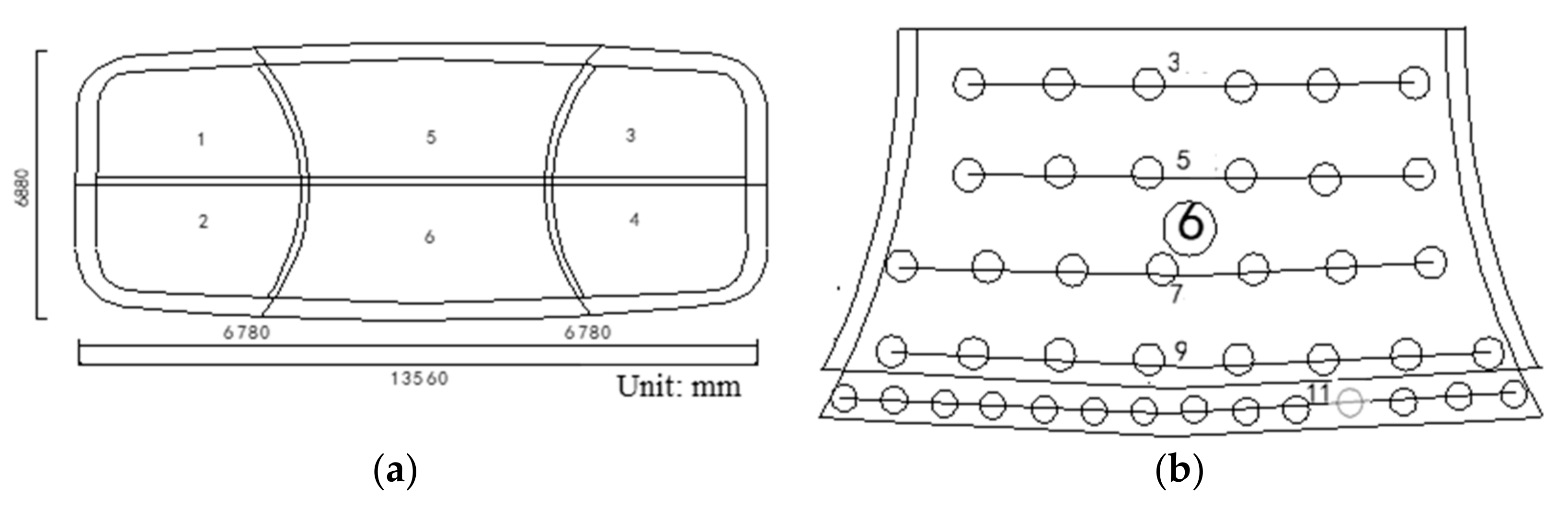
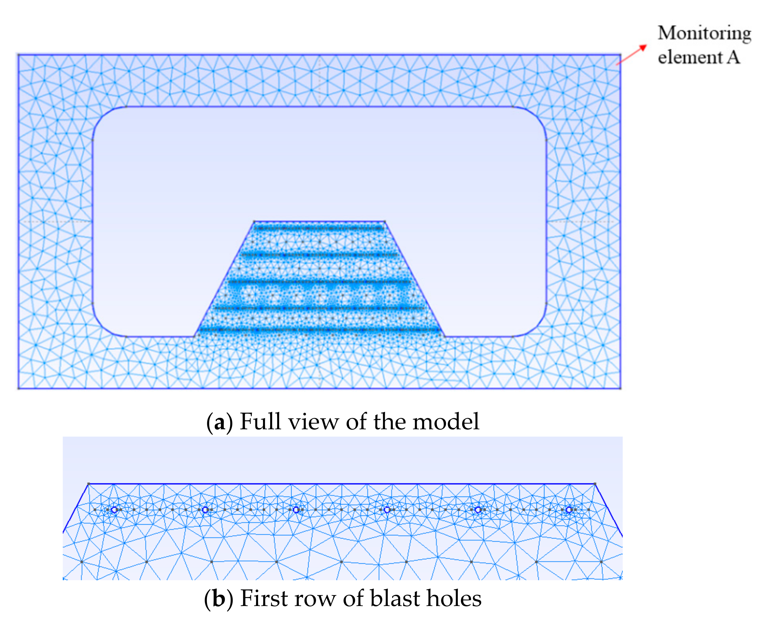
3. Engineering Background

With the rapid development of urban construction in Wuhan, the existing drainage system cannot meet the regional drainage needs. Especially along Guanggu Avenue, the terrain is low-lying. The existing drainage box has been neglected in management for a long time, resulting in serious siltation. In addition, the catchment area of the drainage system along the line is large, and the rainwater cannot be discharged in time during rainstorms, resulting in serious water stagnation in this area. Therefore, the construction of the drainage channel project from Guanggu 1st Road to Gaoxin 4th Road needs to be urgently carried out to improve the drainage and waterlogging prevention capacity of the Guanggu area.

The drainage channel project from Guanggu 1st Road to Gaoxin 4th Road is constructed by the Wuhan Municipal Construction Group. The starting point of the drainage channel project is the intersection of Guanggu 1st Road and Huanglongshan North Road. The construction line runs south along the planned drainage corridor belt on the west side of Guanggu 1st Road; crosses Huanglongshan, the Third Ring Road, and the small intersection overpass of T1\T2 line; and then reaches Gaoxin 4th Road, with a total length of 2.3 km. The section from Ak0 + 135.800 to Ak0 + 887.850 with a length of about 752.050 m is constructed by a concealed excavation method. The cross-sectional shape of the tunnel is a straight wall and a micro-arch. The maximum net width of the tunnel is 13.56 m, the maximum net height is 6.88 m, and the net cross-sectional area is 93.29 m². The standard section shape and size of the tunnel are shown in Figure 4. The surrounding rock of the tunnel crossing includes grades III, IV, and V, and the tunnel blasting excavation construction technology for different surrounding rocks is also different. A variety of excavation methods are adopted in the project, such as the bench method, CRD method, reserved core soil method, and double side drift method. It can be seen that the structure and blasting excavation construction technology of the tunnel are complex, and the transformation of different blasting excavation construction technologies is frequent, which makes the tunnel construction risk high. In addition, the important structures and pipelines around the underground tunnel are densely distributed, resulting in many unforeseen risk factors. The tunnel passes through the Third Ring Road foundation and high-pressure gas pipeline, the existing Huanglongshan Municipal Tunnel, and other important structures at a short distance. The disturbance effect of adjacent construction is significant, and the risk to the surrounding environment is high.

Given the complexity of the geological conditions, the tunnel structure, the surrounding environment, and the blasting excavation construction technology of the project, it is necessary to investigate the deformation mechanism and control of the tunnel excavation under complex conditions, which can provide a scientific basis and technical support for the design and construction of the project. In this paper, the FDEM-based MultiFracS software is used to simulate the tunnel blasting excavation. It does not need to track crack propagation and mesh re-division when simulating the crack initiation and propagation. Combined with efficient contact detection algorithms and contact force algorithms, the blasting process of rock and soil mass can be modeled accurately. Therefore, the process of complex fracture, fragmentation, movement, and accumulation of rock and soil mass of the blasting excavation can be simulated.

4. Millisecond Delay Determination

To improve the contrast of the analysis, the five blast holes segments (3, 5, 7, 9 and 11, see Figure 5b) of the sixth part (other parts are labeled as 1, 2, 3, 4 and 5, see Figure 5a) of the double side drift method are selected. The numbers in Figure 5 indicate the sequence of excavation or detonation. The differential millisecond delay interval is set between the segments, and the charge arrangement is shown in Figure 5b. The transverse direction of the tunnel is the X-axis, and the Y-axis is the vertical direction. According to the actual engineering conditions, the size of the model is 18 × 10 m, and the size of the tunnel is 13.56 × 6.88 m. Gmsh software is used to build models and generate the computational mesh, as shown in Figure 6. In the FDEM, the numerical simulation results are affected by the mesh size. When the mesh size is small enough, the FDEM numerical simulation results tend to be stable [35,43]. Therefore, using a small mesh size does not have a significant effect on the peak blasting vibration velocity. The normal direction around the model is fixed and set as absorbing boundaries. The values of the millisecond delay are 5, 10, 20, 30, 40, and 50 ms, respectively. By simulating these six working conditions, the peak blasting vibration velocity of the monitoring element on the right boundary of the model in Figure 6 is obtained. Then, the influence of a different millisecond delay on the peak blasting vibration velocity is analyzed to obtain a reasonable millisecond delay interval, which provides a reference for the selection and optimization of a reasonable millisecond delay. According to engineering experience and data, the meso-parameters input during calculation are shown in

Table 1. Meso input parameters of MultiFracS for tunnel calculation model.

Parameters	Value
Triangular element
$\mathrm{Density}$ (kg/m3)	2300
Elastic Modulus E (GPa)	20
Friction angle (°)	30
$\mathrm{Normal} \mathrm{contact} \mathrm{penalty} \mathrm{parameter} p_n$ (GPa)	2000
$\mathrm{Tan}\mathrm{gential} \mathrm{contact} \mathrm{penalty} \mathrm{parameter} p_t$ (GPa/m)	2000
$\mathrm{Poisson}$	0.25
Joint element
$\mathrm{Cohesive}$ (MPa)	1.5
$\mathrm{Tensile} \mathrm{strength} f_t$ (MPa)	14
$\mathrm{Internal}$ (°)	30
$\mathrm{Tensile} \mathrm{break} \mathrm{energy} \mathrm{release} \mathrm{rate} G{f}_{{\rm I}}$ (J/m2)	30,000
$\mathrm{Shear} \mathrm{fracture} \mathrm{energy} \mathrm{release} \mathrm{rate} G{f}_{{\rm I}{\rm I}}$ (J/m2)	100,000
Blasting load peak (surrounding holes/other holes) MPa	104/316

.

As shown in Figure 7, the exponential blasting load function $P(t)$ is applied to the blast hole [44]:

$$P(t)=P_0(e^{-\alpha t}-e^{-\beta t})/(e^{-\alpha t_0}-e^{-\beta t_0})$$

(14)

where $t_0$ is the load rise time, which can be obtained by $t_0=[1/(\beta -\alpha )]\log (\beta /\alpha )$, and $\beta /\alpha$ is the control parameter of pressure decay. In this study, $\beta /\alpha =100$ and $t_0$ = 10 μs are selected for simulation. $P(t)$ only acts on the initial surface of the blast holes. Therefore, the gas flow into the crack is not considered. $P_0$ is the peak load, which is obtained from the blasting technical parameters [45]. The peak load acting on the cutting holes, auxiliary holes, and bottom plate holes is all 316 MPa, and the peak load acting on the peripheral blast holes is 104 MPa.

Figure 8 shows that the blasting vibration velocity of monitoring element A under different millisecond delays calculated by MultiFracS software. The main shock phases of the blasting vibration velocity waveforms basically overlap when the millisecond delay is 5 ms. With the increase in the differential millisecond delay, the main shock phases generated by different blast holes are gradually separated, and the superposition effect of the blasting vibration gradually weakens. Four peaks are formed without considering the peripheral blast holes. The main shock phases are completely separated when the millisecond delay is 50 ms, and the blasting vibration waveforms caused by the four blast holes can be clearly observed in the Figure 8.

In addition, the peak blasting vibration velocity of each segment obtained by the monitoring element is different. When the millisecond delay is 5 ms, the peak blasting vibration velocity of the particle is the largest, and the blasting vibration velocity is 2.304 cm/s. When the millisecond delay is 20 ms, the peak blasting vibration velocity of the particle is the smallest, and the blasting vibration velocity is 1.483 cm/s. The millisecond delay affects the blasting vibration waveform caused by subsequent blast holes. For example, after the second blast hole is detonated, the peak blasting vibration velocity of the monitoring element is 1.095 and 1.008 cm/s, respectively, when the millisecond delay is 20 and 30 ms. It is significantly lower than the other groups of blast holes in the same segment. After the third and fourth blast holes are detonated, the peak blasting vibration velocity will decrease with the increase in the millisecond delay and finally tend to be a stable value. Therefore, we can find that the influence of the millisecond delay on the peak blasting vibration velocity is not a single positive correlation or negative correlation. But when the millisecond delay is greater than 40 ms, the millisecond delay does not affect the peak blasting vibration velocity. In summary, the blasting vibration velocity effect is the best when the millisecond delay is 20–30 ms, and it meets the requirements of the project that the blasting vibration velocity is less than 2 cm/s. Therefore, the millisecond delay will be set to 20 ms in the subsequent simulation.

5. Various Blasting Excavation Construction Technologies

A numerical model considering the near-field fracture process of the tunnel surrounding rock is established based on the actual engineering geology. However, it is difficult to establish the same model as the reality. Therefore, the numerical model is simplified as much as possible to reduce the computational burden. The last construction process of the three blasting excavation construction techniques is simulated (the double side drift method, the reserved core soil method, and the CRD method, as shown in Figure 9). The numbers in Figure 9 indicate different excavation sequences. The transverse direction of the tunnel is the X-axis, and the Y-axis is the vertical direction. According to the actual engineering conditions, the size of the model is 18 × 10 m, and the size of the tunnel is 13.56 × 6.88 m. The mesh of the model is shown in Figure 10. The normal direction around the model is fixed and set as absorbing boundaries. The calculation parameters are consistent with Table 1 except that the tensile and shear fracture energy release rates are 300 and 1000, respectively. The blasting load P(t) adopts the same parameters as Section 4.

The rock fracture process of the tunnel surrounding under three different blasting excavation construction techniques is shown in Figure 11, Figure 12 and Figure 13. The blasting rock splashes toward the free surface in the calculation process. Figure 11 shows the fracture and fragmentation process of the double side drift method, and the sequential millisecond blasting method between rows parallel to the contour of the tunnel bottom is adopted. Figure 12 shows the fracture and fragmentation process of the reserved core soil method, and Figure 13 shows the fracture and fragmentation process of the CRD method, which adopts the ladder millisecond blasting method. Cracks first appear around the blast holes, then extend outward, and finally penetrate each other between the blast holes. The crack penetration shape is consistent with other numerical methods and actual construction as shown in Figure 14, (The number in Figure 14b represents the serial number of the cracks.), which verifies the effectiveness of the MultiFracS software in dealing with the tunnel blasting process.

However, the crack morphology of different blasting excavation construction techniques is different. As shown in Figure 12, cracks initiated by the front blast hole extend to the unexploded peripheral blast hole after the blasting of the third segment blast hole, which weaken the directional fracture control effect of the peripheral blast hole, resulting in the lack of integrity and flatness of the excavation surface of the peripheral blast hole in 201 ms. As shown in Figure 13, the peripheral blast hole will detonate at 161 ms. Compared with other blasting excavation construction techniques, there is no effective void effect between the blast holes of the peripheral blast holes of the CRD method, which represents that the surrounding rock around the blast holes is not effectively broken. It may be caused by the high strength of the surrounding rock or the large spacing between the blast holes.

Figure 15 shows the displacement distribution and rock fracture and fragmentation process using the double side drift method excavation model. The first segment of the blast hole is detonated at 0.1 ms. The surrounding rock around the blast hole begins to move under the blasting load and the displacement of the surrounding rock around the blast hole is 0.002 m. At 1.0 ms, the displacement of the surrounding rock around the blast hole close to the free surface increases continuously, and the displacement of the surrounding rock around the blast hole far away from the free surface increases slowly. The surrounding rock near the free surface above the first segment of the blast hole is completely broken and splashed around at 20.5–34.0 ms. The surrounding rock below the blast hole of the first segment blast hole is subjected to the blasting load of the second segment blast holes at this moment. The displacement increases continuously, resulting in an upward-lifting trend. The surrounding rock around the second segment of the blast hole produces horizontal cracks that penetrate each other and gradually form a complete excavation surface. The similar fracture mode is obtained in the fracture process of the surrounding rock around the third segment blast hole (42.0–49.0 ms), the fourth segment blast hole (62.0–69.0 ms), and the fifth segment blast hole (80.5–83.0 ms). The surrounding rocks between the peripheral blast holes basically penetrated each other at 83.0 ms. The surrounding rock above the peripheral blast holes reaches the maximum displacement of 0.005 m at this moment, and the displacement of the surrounding rock below the peripheral blast holes basically tends to 0. Therefore, the integrity and flatness of the tunnel excavation surface can be ensured.

Figure 16 shows the stress–time curves of the monitoring element under different blasting excavation construction techniques. The monitoring element is consistent with monitoring element A mentioned in Section 4. It can be seen from Figure 16 that the peak stress range of the monitoring element under the double side drift method is 0.4–0.5 MPa, the reserved core soil method is 0.1–0.4 MPa, and the CRD method is 0.2–0.7 MPa when each segment of the blast hole is detonated. Compared with the reserved core soil method and the CRD method, the stress change under the double side drift method is uniform. The peak stress of the CRD method is the highest. The difference of the peak stress produced by the peripheral blast holes detonation under different blasting excavation construction techniques is small.

6. Conclusions

In this paper, a numerical study of the blasting excavation process is carried out using the FEDM-based MultiFracS software. Combined with the drainage channel project of Guanggu 1st Road to Gaoxin 4th Road, the numerical model considering the near-field fracture process is studied, and the influence of different millisecond delay and blasting excavation construction technologies on the fracture and the blasting vibration velocity of the surrounding rock around the blast hole is investigated. According to the numerical simulation results, the following conclusions can be drawn:

(1)

The influence of the millisecond delay on the peak blasting vibration velocity is not a single positive correlation or negative correlation, but when the millisecond delay is greater than 40 ms, the delay time no longer affects the peak blasting vibration velocity. When the millisecond delay is 20–30 ms, the peak blasting vibration velocity is the smallest, and it meets the requirements of the project that the blasting vibration velocity is less than 2 cm/s.

(2)

Through the numerical simulation on the near-field surrounding rock fracture of the drainage channel project from Guanggu 1st Road to Gaoxin 4th Road, the optimal blasting excavation construction technology of grade III surrounding rock is the double side drift method. It has a better control effect on the deformation and crushing of the surrounding rock of the tunnel.

(3)

Not only can the MultiFracS software simulate the whole process of a complex fracture, fragmentation, and movement of rock and soil during blasting and excavation, but it can provide information on the evolution of the displacement field and stress field in the process of blasting, which provides a powerful simulation tool for blasting and excavation engineering.

References

1. Ramulu, M.; Chakraborty, A.K.; Sitharam, T.G. Damage assessment of basaltic rock mass due to repeated blasting in a railway tunnelling project—A case study. Tunn. Undergr. Space Technol. 2009, 24, 208–221. [Google Scholar] [CrossRef]
2. Kim, E.; Stine, M.A.; de Oliveira, D.B.M. Effects of water content and loading rate on the mechanical properties of Berea Sandstone. J. South. Afr. Inst. Min. Metall. 2019, 119, 1077–1082. [Google Scholar] [CrossRef]
3. Singh, R.K.; Sawmliana, C.; Hembram, P. Damage threat to sensitive structures of a thermal power plant from hard rock blasting operations in track hopper area: A case study. Int. J. Prot. Struct. 2020, 11, 3–22. [Google Scholar] [CrossRef]
4. Villaescusa, E.; Neindorf, L.B. Damage to stope walls from underground blasting. In Proceedings of the 6th International Conference on Structures under Shock and Impact (SUSI VI), Cambridge, UK, 3–5 July 2000; pp. 129–140. [Google Scholar]
5. Tao, M.; Li, X.; Wu, C. 3D numerical model for dynamic loading-induced multiple fracture zones around underground cavity faces. Comput. Geotech. 2013, 54, 33–45. [Google Scholar] [CrossRef] [Green Version]
6. Liu, X.; Song, S.; Tan, Y.; Fan, D.; Ning, J.; Li, X.; Yin, Y. Similar simulation study on the deformation and failure of surrounding rock of a large section chamber group under dynamic loading. Int. J. Min. Sci. Technol. 2021, 31, 495–505. [Google Scholar] [CrossRef]
7. Saiang, D.; Nordlund, E. Numerical Analyses of the Influence of Blast-Induced Damaged Rock Around Shallow Tunnels in Brittle Rock. Rock Mech. Rock Eng. 2008, 42, 421–448. [Google Scholar] [CrossRef]
8. Li, X.; Cao, W.; Zhou, Z.; Zou, Y. Influence of stress path on excavation unloading response. Tunn. Undergr. Space Technol. 2014, 42, 237–246. [Google Scholar] [CrossRef]
9. Yang, J.H.; Yao, C.; Jiang, Q.H.; Lu, W.B.; Jiang, S.H. 2D numerical analysis of rock damage induced by dynamic in-situ stress redistribution and blast loading in underground blasting excavation. Tunn. Undergr. Space Technol. 2017, 70, 221–232. [Google Scholar] [CrossRef]
10. Xie, L.X.; Lu, W.B.; Zhang, Q.B.; Jiang, Q.H.; Wang, G.H.; Zhao, J. Damage evolution mechanisms of rock in deep tunnels induced by cut blasting. Tunn. Undergr. Space Technol. 2016, 58, 257–270. [Google Scholar] [CrossRef]
11. Munjiza, A.; Andrews, K.; White, J.K. Combined single and smeared crack model in combined finite-discrete element analysis. Int. J. Numer. Methods Eng. 1999, 44, 41–57. [Google Scholar] [CrossRef]
12. Munjiza, A.A. The Combined Finite-Discrete Element Method; John Wiley & Sons: Chichester, UK, 2004. [Google Scholar]
13. Lisjak, A.; Figi, D.; Grasselli, G. Fracture development around deep underground excavations: Insights from FDEM modelling. J. Rock Mech. Geotech. Eng. 2014, 6, 493–505. [Google Scholar] [CrossRef] [Green Version]
14. Lisjak, A.; Garitte, B.; Grasselli, G.; Müller, H.R.; Vietor, T. The excavation of a circular tunnel in a bedded argillaceous rock (Opalinus Clay): Short-term rock mass response and FDEM numerical analysis. Tunn. Undergr. Space Technol. 2015, 45, 227–248. [Google Scholar] [CrossRef] [Green Version]
15. Ma, G.; Zhang, Y.; Zhou, W.; Ng, T.-T.; Wang, Q.; Chen, X. The effect of different fracture mechanisms on impact fragmentation of brittle heterogeneous solid. Int. J. Impact Eng. 2018, 113, 132–143. [Google Scholar] [CrossRef]
16. Ma, G.; Zhou, W.; Regueiro, R.A.; Wang, Q.; Chang, X. Modeling the fragmentation of rock grains using computed tomography and combined FDEM. Powder Technol. 2017, 308, 388–397. [Google Scholar] [CrossRef]
17. Rougier, E.; Knight, E.E.; Broome, S.T.; Sussman, A.J.; Munjiza, A. Validation of a three-dimensional Finite-Discrete Element Method using experimental results of the Split Hopkinson Pressure Bar test. Int. J. Rock Mech. Min. Sci. 2014, 70, 101–108. [Google Scholar] [CrossRef]
18. Fukuda, D.; Mohammadnejad, M.; Liu, H.; Dehkhoda, S.; Chan, A.; Cho, S.H.; Min, G.J.; Han, H.; Kodama, J.i.; Fujii, Y. Development of a GPGPU-parallelized hybrid finite-discrete element method for modeling rock fracture. Int. J. Numer. Anal. Methods Geomech. 2019, 43, 1797–1824. [Google Scholar] [CrossRef]
19. Hamdi, P.; Stead, D.; Elmo, D. Damage characterization during laboratory strength testing: A 3D-finite-discrete element approach. Comput. Geotech. 2014, 60, 33–46. [Google Scholar] [CrossRef]
20. Yan, C.Z.; Zheng, H. A new potential function for the calculation of contact forces in the combined finite-discrete element method. Int. J. Numer. Anal. Methods Geomech. 2017, 41, 265–283. [Google Scholar] [CrossRef]
21. Yan, C.; Fan, H.; Huang, D.; Wang, G. A 2D mixed fracture–pore seepage model and hydromechanical coupling for fractured porous media. Acta Geotech. 2021, 16, 3061–3086. [Google Scholar] [CrossRef]
22. Yan, C.; Jiao, Y.-Y. A 2D fully coupled hydro-mechanical finite-discrete element model with real pore seepage for simulating the deformation and fracture of porous medium driven by fluid. Comput. Struct. 2018, 196, 311–326. [Google Scholar] [CrossRef]
23. Yan, C.; Zheng, H. Three-Dimensional Hydromechanical Model of Hydraulic Fracturing with Arbitrarily Discrete Fracture Networks using Finite-Discrete Element Method. Int. J. Geomech. 2017, 17, 6. [Google Scholar] [CrossRef]
24. Yan, C.; Gao, Y.; Guo, H. A FDEM based 3D discrete mixed seepage model for simulating fluid driven fracturing. Eng. Anal. Bound. Elem. 2022, 140, 447–463. [Google Scholar] [CrossRef]
25. Yan, C.; Guo, H.; Tang, Z. Three-dimensional continuous-discrete pore-fracture mixed seepage model and hydro-mechanical coupling model to simulate hydraulic fracturing. J. Pet. Sci. Eng. 2022, 215, 110510. [Google Scholar] [CrossRef]
26. Yan, C.; Jiao, Y.-Y.; Zheng, H. A fully coupled three-dimensional hydro-mechanical finite discrete element approach with real porous seepage for simulating 3D hydraulic fracturing. Comput. Geotech. 2018, 96, 73–89. [Google Scholar] [CrossRef]
27. Yan, C.; Tong, Y.; Luo, Z.; Ke, W.; Wang, G. A two-dimensional grouting model considering hydromechanical coupling and fracturing for fractured rock mass. Eng. Anal. Bound. Elem. 2021, 133, 385–397. [Google Scholar] [CrossRef]
28. Yan, C.; Zheng, Y.; Ke, W.; Wang, G. A FDEM 3D moisture migration-fracture model for simulation of soil shrinkage and desiccation cracking. Comput. Geotech. 2021, 140, 104425. [Google Scholar] [CrossRef]
29. Yan, C.; Wei, D.; Wang, G. Three-dimensional finite discrete element-based contact heat transfer model considering thermal cracking in continuous–discontinuous media. Comput. Methods Appl. Mech. Eng. 2022, 388, 114228. [Google Scholar] [CrossRef]
30. Yan, C.; Zheng, Y.; Huang, D.; Wang, G. A coupled contact heat transfer and thermal cracking model for discontinuous and granular media. Comput. Methods Appl. Mech. Eng. 2021, 375, 113587. [Google Scholar] [CrossRef]
31. Yan, C.; Yang, Y.; Wang, G. A new 2D continuous-discontinuous heat conduction model for modeling heat transfer and thermal cracking in quasi-brittle materials. Comput. Geotech. 2021, 137, 104231. [Google Scholar] [CrossRef]
32. Yan, C.; Jiao, Y.-Y. A 2D discrete heat transfer model considering the thermal resistance effect of fractures for simulating the thermal cracking of brittle materials. Acta Geotech. 2019, 15, 1303–1319. [Google Scholar] [CrossRef]
33. Yan, C.; Wang, X.; Huang, D.; Wang, G. A new 3D continuous-discontinuous heat conduction model and coupled thermomechanical model for simulating the thermal cracking of brittle materials. Int. J. Solids Struct. 2021, 229, 111123. [Google Scholar] [CrossRef]
34. Yan, C.; Zheng, H. A coupled thermo-mechanical model based on the combined finite-discrete element method for simulating thermal cracking of rock. Int. J. Rock Mech. Min. Sci. 2017, 91, 170–178. [Google Scholar] [CrossRef]
35. Yan, C.; Fan, H.; Zheng, Y.; Zhao, Y.; Ning, F. Simulation of the thermal shock of brittle materials using the finite-discrete element method. Eng. Anal. Bound. Elem. 2020, 115, 142–155. [Google Scholar] [CrossRef]
36. Yan, C.; Xie, X.; Ren, Y.; Ke, W.; Wang, G. A FDEM-based 2D coupled thermal-hydro-mechanical model for multiphysical simulation of rock fracturing. Int. J. Rock Mech. Min. Sci. 2022, 149, 104964. [Google Scholar] [CrossRef]
37. Yan, C.; Jiao, Y.Y. FDEM-TH3D: A three-dimensional coupled hydrothermal model for fractured rock. Int. J. Numer. Anal. Methods Geomech. 2018, 43, 415–440. [Google Scholar] [CrossRef] [Green Version]
38. Yan, C.; Luo, Z.; Zheng, Y.; Ke, W. A 2D discrete moisture diffusion model for simulating desiccation fracturing of soil. Eng. Anal. Bound. Elem. 2022, 138, 42–64. [Google Scholar] [CrossRef]
39. Yan, C.; Wang, T.; Ke, W.; Wang, G. A 2D FDEM-based moisture diffusion–fracture coupling model for simulating soil desiccation cracking. Acta Geotech. 2021, 16, 2609–2628. [Google Scholar] [CrossRef]
40. Wang, T.; Yan, C.; Wang, G.; Zheng, Y.; Ke, W.; Jiao, Y.-Y. Numerical study on the deformation and failure of soft rock roadway induced by humidity diffusion. Tunn. Undergr. Space Technol. 2022, 126, 104565. [Google Scholar] [CrossRef]
41. Wang, T.; Yan, C.; Zheng, Y.; Jiao, Y.-Y.; Zou, J.J.C. Geotechnics. Numerical study on the effect of meso-structure on hydraulic conductivity of soil-rock mixtures. Comput. Geotech. 2022, 146, 104726. [Google Scholar] [CrossRef]
42. Munjiza, A.; Andrews, K.R.F. NBS contact detection algorithm for bodies of similar size. Int. J. Numer. Methods Eng. 1998, 43, 131–149. [Google Scholar] [CrossRef]
43. Guo, L.; Xiang, J.; Latham, J.-P.; Izzuddin, B. A numerical investigation of mesh sensitivity for a new three-dimensional fracture model within the combined finite-discrete element method. Eng. Fract. Mech. 2016, 151, 70–91. [Google Scholar] [CrossRef] [Green Version]
44. Duvall, W.I.J.G. Strain-wave shapes in rock near explosions. Geophysics 1953, 18, 310–323. [Google Scholar] [CrossRef]
45. Henrych, J.; Abrahamson, G.R. The dynamics of explosion and its use. J. Appl. Mech. 1980, 47, 218. [Google Scholar] [CrossRef]
46. Han, H.; Fukuda, D.; Liu, H.; Fathi Salmi, E.; Sellers, E.; Liu, T.; Chan, A. FDEM simulation of rock damage evolution induced by contour blasting in the bench of tunnel at deep depth. Tunn. Undergr. Space Technol. 2020, 103, 103495. [Google Scholar] [CrossRef]
47. Olsson, M.; Niklasson, B.; Wilson, L.; Andersson, C.; Christiansson, R. Äspö HRL. Experiences of Blasting of the TASQ Tunnel; Swedish Nuclear Fuel and Waste Management Co.: Stockholm, Sweden, 2004. [Google Scholar]
Figure 1. The connection relationship between the triangular element and joint element in FDEM [20].
Applsci 12 07517 g001
Figure 3. (a) Discretization for the contact between blocks with arbitrary shape; (b) contact between triangular elements [11,12].
Applsci 12 07517 g003
Figure 4. Schematic diagram of the cross-sectional shape of the tunnel in the surrounding rock section of grades III, IV, and V.
Applsci 12 07517 g004
Figure 5. (a) Schematic diagram of blasting excavation construction process of the double side drift method; (b) schematic diagram of the blast hole arrangement and networked detonation in part VI.
Applsci 12 07517 g005
Figure 6. Schematic diagram of tunnel calculation model and monitoring unit for the double-side-drift method.
Applsci 12 07517 g006
Figure 7. Pressure–time curve of blasting load waveform.
Applsci 12 07517 g007
Figure 8. The blasting vibration velocity of monitoring element A under different millisecond delays.
Applsci 12 07517 g008
Figure 9. Schematic diagram of tunnel blasting excavation construction technology.
Applsci 12 07517 g009
Figure 10. Schematic diagram of the blasting excavation construction model and the mesh division.
Applsci 12 07517 g010
Figure 11. The fracture and fragmentation process of rock using the double side drift method.
Applsci 12 07517 g011aApplsci 12 07517 g011b
Figure 12. The fracture and fragmentation process of rock damage and fracture in the reserved core soil method.
Applsci 12 07517 g012aApplsci 12 07517 g012b
Figure 13. The process of rock damage and fracture in the CRD method.
Applsci 12 07517 g013aApplsci 12 07517 g013b
Figure 14. Tunnel crack propagation law: (a) other numerical simulation [46]; (b) field test results [47].
Applsci 12 07517 g014
Figure 15. Displacement distribution and rock fracture and fragmentation process using the double side drift method.
Applsci 12 07517 g015aApplsci 12 07517 g015b
Figure 16. Stress and time curve of monitoring element under different blasting excavation construction technologies.
Applsci 12 07517 g016