Article

An Underdetermined Convolutional Blind Separation Algorithm for Time–Frequency Overlapped Wireless Communication Signals with Unknown Source Number

School of Communication Engineering, Army Engineering University of PLA, Nanjing 210007, China
*
Author to whom correspondence should be addressed.
Appl. Sci. 2022, 12(13), 6534; https://doi.org/10.3390/app12136534
Submission received: 30 May 2022 / Revised: 16 June 2022 / Accepted: 24 June 2022 / Published: 28 June 2022
(This article belongs to the Special Issue Advanced Electronics and Digital Signal Processing)

Abstract

:
It has been challenging to separate the time–frequency (TF) overlapped wireless communication signals with unknown source numbers in underdetermined cases. In order to address this issue, a novel blind separation strategy based on a TF soft mask is proposed in this paper. Based on the clustering property of the signals in the sparse domain, the angular probability density distribution is obtained by the kernel density estimation (KDE) algorithm, and then the number of source signals is identified by detecting the peak points of the distribution. Afterward, the contribution degree function is designed according to the cosine distance to calculate the contribution degrees of the source signals in the mixed signals. The separation of the TF overlapped signals is achieved by constructing a soft mask matrix based on the contribution degrees. The simulations are performed with digital signals of the same modulation and different modulation, respectively. The results show that the proposed algorithm has better anti-aliasing and anti-noise performance than the comparison algorithms.

1. Introduction

1.1. Research Background and Motivation

Blind source separation (BSS), defined as the task of separating the source signals from the observed signals when the source signals and the mixing mode are not known exactly, enables the separation of the mixed signals and the extraction of the source signals without a priori knowledge. As a kind of front-end technology in the field of signal processing, the BSS is of great importance in communication anti-jamming and improving spectrum utilization [1]. Unfortunately, the classical independent component analysis (ICA) and many extended algorithms [2,3,4] are based on the main assumption that the number of observed signals is greater than or equal to the number of source signals, which cannot realize the blind signal separation in underdetermined cases [5]. In practical communication scenarios, the number of observed signals is usually less than the number of source signals on account of system cost or environmental constraints, thus the study of underdetermined blind source separation (UBSS) is of more practical significance. At present, the main approach to tackle the issue of UBSS is based on sparse component analysis (SCA) [6]. The main strategy of the SCA method is solving the UBSS by exploiting the sparsity of the source signal or sparsity in the transform domain. However, with the dramatic increase in RF devices, it is almost inevitable that signals will be overlapped in the time and frequency domains. For communication signals that are not completely sparse in the time and frequency domains, it has been a challenge to solve the UBSS problem using the SCA method. It is of practical importance to separate the TF overlapped signals in underdetermined cases. This paper aims to improve the SCA algorithm for the effective separation of TF overlapped wireless communication signals with unknown source numbers.

1.2. Literature Review

The classical SCA algorithm mainly consists of the two-stage method and the TF masking method. The two-stage method first estimates the mixing matrix and then uses signal sparsity to recover the source signal. Zhen [7] utilized the sparse coding technique to discover the 1-D subspace from the set of TF points, then estimated the mixing matrix by grouping vectors in the subspace through hierarchical clustering, and finally used the least-squares method to achieve source signal recovery; Fang [8] firstly estimated the mixing matrix based on the hyperplane normal vector clustering algorithm, and then used the classical algorithm called orthogonal matching pursuit in compressed sensing to realize the separation of the linear frequency modulated radar mixed signals; Fu [9] realized the recovery of the source signal using a new subspace complementary matching pursuit algorithm. The algorithm reduced the computational complexity by selecting multiple atoms per iteration and also used L 2 parametric minimization instead of L 0 parametric minimization in order to improve the recovery accuracy.
The other is the TF masking method, i.e., the source signal is separated by designing a TF mask matrix. Yu [10] first detected the peak energy point of the mixed signals and then calculated the cosine distance between all energy points and the peak energy point, afterward obtained the binary mask based on a threshold to realize the reconstruction of the vibration signal; Cobos [11] proposed a maximum a posteriori decision criterion to design a binary mask matrix for the separation of mixed speech signals; Kumar [12] first detected the active single-source points by calculating the mixing ratio, and then found the cluster centers by a dynamic routing algorithm as a way to design a binary mask.
The above algorithms usually assume that the signal is sparse in some domains, such as the time domain, frequency domain, etc. However, in the wireless communication scenarios, the signals are inevitably overlapped in both time and frequency domains. In such cases, it may cause a reduction in separation accuracy or even complete failure when the classical SCA-based method is applied directly to the separation of TF overlapped communication signals. The two-stage method could not guarantee the estimation accuracy of the mixing matrix and the performance of the source signal recovery, while reconstructing the source signals through the TF binary mask will bring certain distortions [13,14,15]. Obviously, for the communication mixed signals with TF aliasing, better separation performance can be obtained by reasonably estimating the TF soft mask to reconstruct the source signals [16].

1.3. Contribution and Paper Organization

Under the framework of the TF masking method, we propose a novel underdetermined convolutional mixing UBSS algorithm for TF overlapped communication signals with an unknown number of sources. Firstly, the observed signals are converted to the sparse domain to obtain the linear clustering characteristic. Consequently, the effects of multipath and time delay are eliminated by calculating short-time spectral power; Secondly, the short-time spectral power ratio of the observed signals is converted into the angular distribution, and the number of source signals can be estimated through the KDE algorithm; Then the contribution degree of the source signal in the observed signal is obtained by the designed contribution degree function. Finally, the TF soft mask is constructed based on the contribution degree, which is employed to separate the mixed signals. The main contribution of the paper can be summarized in the following:
  • A source number estimation method based on the KDE algorithm followed by detecting the peak points of the distribution is proposed, which can effectively estimate the number of sources before the signal separation.
  • We design a contribution degree function based on the cosine distance, by which the contribution degree of the source signal to the mixed signal can be obtained. The contribution degree clearly reflects the mixing degree of the source signal at each frequency point, and it is of significant importance to improve the separation accuracy.
  • The TF soft mask matrix is constructed based on the contribution degree function. Compared with the traditional binary mask, the TF soft mask can improve the separation accuracy for TF overlapped signals.
  • The proposed blind source separation method for TF overlapped communication signal extends the application of the SCA algorithm, which reduces the requirement of signal sparsity for the classical SCA blind source separation algorithm.
The rest of this paper is structured as follows. The problem statement is given in Section 2, which includes the introduction of the effect on separation based on the classical SCA methods caused by TF aliasing. Subsequently, Section 3 describes the process of the algorithm in detail, which mainly consists of two parts: source number estimation and source signal recovery. Afterward, the separation performance of this algorithm is tested by the simulations in Section 4. Lastly, the conclusions are drawn in Section 5.

2. Problem Statement

In the wireless communication propagation model, multipath and time delay of signals are inevitable, which can be modeled as the convolutive mixture of the source signals [17]. All variables involved in the problem statement are described in Table 1. Without considering the noise, the mathematical expression of the convolutional mixture model can be expressed as
x ( t ) = q = 1 Q A q s ( t )
where s ( t ) represents the source signal; x ( t ) indicates the received mixed signal; Q is the number of wireless propagation paths; A q denotes the mixing matrix corresponding to the qth path. Considering the effect of time delay. A q can be expressed as
A q = [ a 11 q δ ( t τ 11 q ) a 12 q δ ( t τ 12 q ) a 1 n q δ ( t τ 1 n q ) a 21 q δ ( t τ 21 q ) a 22 q δ ( t τ 22 q ) a 2 n q δ ( t τ 2 n q ) a k i q δ ( t τ k i q ) a m 1 q δ ( t τ m 1 q ) a m 2 q δ ( t τ m 2 q ) a m n q δ ( t τ m n q ) ]
where δ ( · ) represents the impulse response, a k i q and τ k i q are the amplitude attenuation and time delay of the ith source signal to the kth sensor through the qth path, respectively. In order to obtain the sparse characteristic of the signals, the signal X k ( t , f ) received by the kth sensor after a short-time Fourier transform (STFT) [18] can be written as
X k ( t , f ) = i = 1 n q = 1 Q a k i q S i q ( t τ k i q , f )
Take the BPSK signal as an example; the TF expression is described as
X k ( t , f ) = i = 1 n q = 1 Q a k i q h ^ ( f ± f i ) e j 2 π f i ( t τ k i q )
where f i denotes the center frequency of the ith source signal. After performing the modulus operation on X k ( t , f ) [19], the power P k ( f ) of the kth received signal can be expressed as
P k ( f ) = + | X k ( t , f ) | d t = | i = 1 n q = 1 Q a k i q h ^ ( f ± f i ) | + | e j 2 π f i ( t τ k i q ) | d t = | i = 1 n q = 1 Q a k i q h ^ ( f ± f i ) |
where | · | expresses modulus operation. When the spectrum of the source signal is non-aliased, there is only the component of the source signal s i ( t ) in the interval [ f i Δ , f i + Δ ] ( Δ > 0 ) of the received signal. In this case, the power ratio P α ( f ) / P β ( f ) of any two of the received signals X α and X β is
P α ( f ) / P β ( f ) = | i = 1 n q = 1 Q a α i q h ^ ( f ± f i ) | | i = 1 n q = 1 Q a β i q h ^ ( f ± f i ) | = | q = 1 Q a α i q | | q = 1 Q a β i q | , f [ f i Δ , f i + Δ ]
Consequently, the short-time spectral power points of the signal s i ( t ) will be clustered on the line with a slope of P α ( f ) / P β ( f ) . Figure 1 represents the scatter plot of the power ratio of the two received signals after the convolutive mixture of the four BPSK signals. Due to the sparsity of the observed signals in the power domain, the received signals exhibit linear clustering property. There are four linear clusters in Figure 1 corresponding to the four source signals, and thus the mixed signals can be effectively separated by the traditional single-source-point (SSP) detection method [10]. However, in practical communication systems, it is almost impossible to avoid TF aliasing for communication signals. When the spectrum of the source signal is overlapped, the sparsity of the observed signals in the power domain cannot be guaranteed, thus weakening the linear clustering property of the observed signals (Figure 2). The traditional SSP method will not accurately recover the source signal.

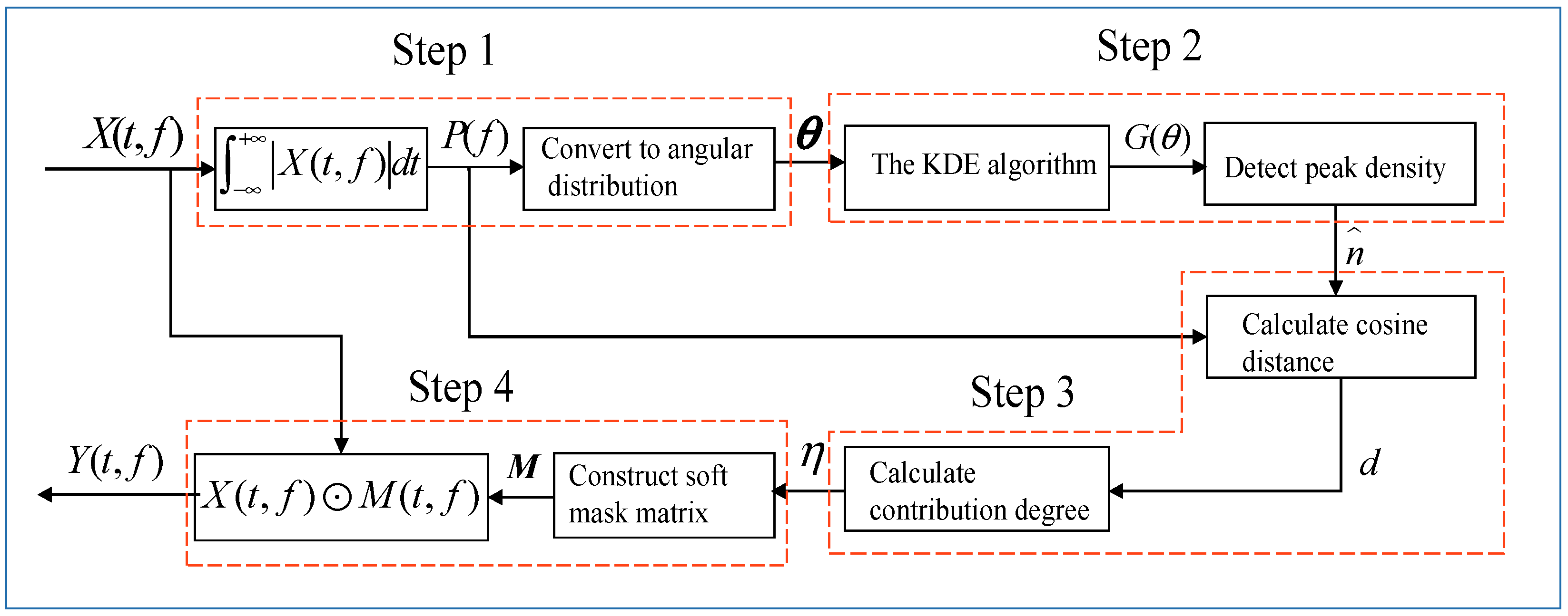
3. UBSS Algorithm Based on TF Soft Mask

To tackle the above challenge, we propose a new blind separation strategy based on TF soft mask. The process consists of two main stages. The first step is to determine the number of sources through the KDE algorithm, followed by peak detection. After that, the contribution degree of the source signal in the observed signal is calculated by the contribution degree function to construct the TF soft mask matrix, which is used to separate the TF aliasing signals. All variables involved in the section are described in Table 2.

3.1. Source Number Estimation

In the problem of UBSS, the source number estimation is an indispensable step. The accurate estimation of the number of sources is the prerequisite for precise source signal recovery [20,21]. In order to estimate the number of sources accurately, the KDE algorithm is used to calculate the angular probability density distribution of the mixed signal in the sparse domain, followed by detecting the number of peak points of the distribution. In order to eliminate the interference of noise on the signal, a threshold ε needs to be set to screen out the low power points. The set of frequencies F after removing the low power points can be obtained by
F = { f | k = 1 m P k ( f ) > ε max f [ k = 1 m P k ( f ) ] }
where ε is the empirical parameter, which is taken as 0.1 in this paper. In the later expressions, f u is used to denote the uth element of F . Afterward, convert the filtered power points into angular distribution θ :
θ u = arctan [ P α ( f u ) / P β ( f u ) ]
The statistical histogram after converting to an angular distribution is shown in Figure 3. As seen from the figure, the angular distribution is more densely distributed around the intervals 0.07, 0.52, 1.15, and 1.48 than the other intervals. Thus the angular distribution θ is modeled based on the KDE algorithm [22]:
G κ ( θ ) = 1 l u = 1 l K κ ( θ θ u )
where G κ ( θ ) denotes the angular probability density distribution of θ ; l is the length of the vector θ ; K κ ( · ) represents the kernel function with a smoothing factor κ of the bandwidth. In this paper, we choose the Gaussian kernel as the kernel function and take κ as 0.25. The angular probability density distribution obtained by the KDE algorithm is shown in Figure 4. The number of peak points of the angular probability density distribution is the number of sources to be estimated. As we can see from Figure 4, there are four peak points marked by red circles, which means that the number of estimated source signals n ^ is four.

3.2. Source Signal Recovery by TF Soft Mask

Ideally, the reconstruction of the source signal is achieved by inverse short-time Fourier transform (ISTFT) in the frequency band [ f i Δ , f i + Δ ] 10. However, the traditional clustering method is only a kind of hard segmentation of power points to obtain the TF binary mask. When the frequency spectrum is overlapped, the short-term spectral power of the observed signals is the superposition of the short-term spectral power of the source signals. The integrity of the source signal reconstruction cannot be guaranteed through the method of hard segmentation. Thus a matching soft mask matrix M ( t , f ) is required to fully recover the source signal.
Y i ( t , f ) = X ( t , f ) M i ( t , f )
where represents the Hadamard product; Y i ( t , f ) denotes the ith signal to be reconstructed, and M i ( t , f ) is the corresponding TF soft mask matrix that needs to be constructed.
In this paper, the construction of the TF soft mask matrix is performed by designing a contribution degree function based on the cosine distance. It can be seen from Figure 2 that among all the power points inside the ith linear cluster, the endpoint is subject to the least interference. That is, when f u = f i , the contribution degree η u i of the ith source signal to the mixed signal can be taken as 1, and the cosine distance between the endpoint and itself is 1 as well ( f i is the frequency corresponding to the endpoint of the ith linear clustering cluster). When f u is further away from f i , the contribution degree η u i will be decreased. The corresponding cosine distance d u i between the power point and the ith endpoint is decreased as well. Extremely, η u i is taken as 0 when f u is the frequency of the nearest adjacent endpoint. Hence the contribution degree η u i can be characterized by the cosine distance between all power points and the endpoint of the ith linear cluster. A monotonically increasing contribution function is designed to characterize the positive correlation between contribution degree η u i and cosine distance d u i :
η u i = { 1 , d u i = 1 ( d u i d i 1 d i ) γ , 0 < d u i < d i 0 , o t h e r w i s e
where d i denotes the maximum of the cosine distance between the endpoint of the ith linear cluster and the endpoints of the remaining linear clusters; γ denotes the scaling factor of the contribution function, whose different values will affect the separation performance of the algorithm. In Section 4.1, we will discuss the impact of γ on separation performance. The cosine distance of the uth power point from the endpoint of the ith linear cluster d u i is obtained as
d u i = C D { [ P α ( f i ) , P β ( f i ) ] , [ P α ( f u ) , P β ( f u ) ] }
where C D denotes the cosine distance between two points. The frequencies corresponding to the endpoints of the clustering clusters can be detected by seeking the first n ^ peak points in the sum of the power data marked in red Figure 5. The points marked in red are the endpoints of the detected linear clusters to be determined in Figure 6. Therefore, the contribution degree of the uth point to the ith linear cluster can be calculated by the contribution degree function given above.
Based on the contribution degree η u i obtained from Equation (11), the ith TF soft mask matrix M i is constructed by the following formula:
M i = [ η 1 i η 2 i η F i η 1 i η 2 i η F i η 1 i η 2 i η F i ] T × F
where F is the number of STFT frequencies; T is the number of time series of STFT. n ^ soft mask matrices can be constructed in this way.
The ith source signal y i ( t ) to be reconstructed is
y i ( t ) = I S T F T [ X ( t , f ) M i ( t , f ) ]
where X ( t , f ) indicates the sum of the observed signals.
The flowchart of the proposed strategy is shown in Figure 7. Firstly, the angular distribution θ is converted from the power ratio by Equation (8); Secondly, the number of source signals n ^ is estimated through the KDE algorithm followed by the peak density detection; Afterwards, the contribution degree η of the source signal in the observed signal is calculated by the contribution degree function based on the cosine distance d . Finally, the TF soft mask matrix M is constructed based on the contribution degree η , and the separated TF signals are reconstructed.

4. Experimental Results and Analysis

Our simulations are aimed at investigating the anti-aliasing performance and anti-noise performance of the proposed algorithm. To measure the degree of spectrum aliasing of the source signals, we define the degree of spectrum aliasing λ :
λ = B o B × 100 %
where B represents the source signal spectrum bandwidth, B o and represents the maximum aliasing width between the source signal spectrum and the adjacent signal spectrum.
Since the “boundary effect” of STFT has an impact on the separation performance [10], we selected the Kaiser window ( β = 6.865 ) as the window function. The evaluation criteria of separation performance were applied in our simulations, which include the source-to-distortion ratio (SDR), the source-to-interferences ratio (SIR), the source-to-artifacts ratio (SAR) [23], and the separated bit error rate (BER). In order to obtain bitstream information, the coherent demodulation method was used to demodulate the separated source signals. The mixed signals were separated by the SCA algorithm proposed in this paper and the literatures [8,10]. The comparison algorithm in [8] belonged to the classic two-stage method, and [10] used the TF masking method to separate the source signal.

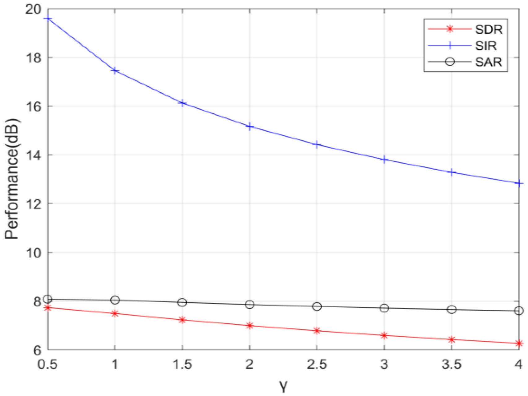
4.1. Simulation 1: The Selection of Scaling Factor γ in the Contribution Degree Function

In this simulation, we verified the impact of the scaling factor γ on the separation performance of the proposed algorithm. The simulation was conducted under the condition of additive white Gaussian noise with a signal-to-noise ratio (SNR) of 16.4 dB. It is assumed that the three signals with different modulation (2ASK/BPSK/QPSK) are mixed instantaneously, in which the symbol rate of the signals are 5 × 10⁶, 5 × 10⁶, 10 × 106 B, respectively. The modulation carrier frequencies are 13.5, 20, and 26.5 MHz, respectively, with the λ of each signal being 35%. The mixing matrix A is
A = [ 0.21 0.63 0.89 0.92 0.58 0.22 ]
The separation performance with different γ is shown in Figure 8; the bigger value is, the better the separation performance is. It can be seen that, with γ increasing, the SIR decreased significantly while the SAR and SDR remained almost constant. Thus we take γ as 0.5 in the following simulation experiments. Figure 9 and Figure 10 show the waveforms of the source signals and their mixed signals, respectively. Comparatively, Figure 11 shows the waveforms of the signals separated by the proposed algorithm with γ = 0.5 . It can be seen that the waveforms of the separated signals are basically consistent with the source signals. Although the waveforms have some distortion at the junction of bit 0 and bit 1, which is caused by the “boundary effect” of STFT, it does not affect the subsequent demodulation and judgment. Figure 12 represents the waveforms after coherent demodulation. The bit data can be recovered by setting the appropriate judgment level.

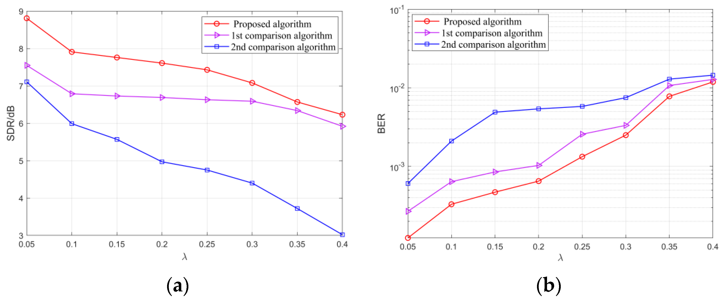
4.2. Simulation 2: The Anti-Aliasing Performance Simulation

In order to analyze the anti-aliasing performance for signals with different modulation methods, two sets of signals were used as the source signals, which respectively were three signals with the same BPSK modulation and three signals with different modulation (2ASK/BPSK/QPSK). The symbol rate of a single source signal is 5 × 10⁶ B. The modulation carrier frequencies were designed according to different λ . In this simulation, it is assumed that the source signals propagate in two channels before being received by the sensors, and the SNR is 15 dB. The first channel of signals arrived instantaneously, and the corresponding mixing matrix is
A 1 = [ 0.23 0.32 0.52 0.44 0.47 0.13 ]
The second channel of signals arrived with delay; the signal propagation delay matrix and the corresponding mixing matrix are
T = [ 0.1 0.05 0.2 0.18 0.1 0.04 ]
A 2 = [ 0.22 0.42 0.37 0.41 0.17 0.28 ]
The SDR and BER of the separated signals with the increase in λ are shown in Figure 13 and Figure 14. From the simulation results, it can be seen that in the environment with the SNR of 15 dB, as the source signal spectrum aliasing gradually intensifies, the separation performance of the proposed algorithm and the comparison algorithms are reduced to varying degrees. However, for signals with the same BPSK modulation (Figure 13), the average SDR of the separated signals by the proposed algorithm is increased by 1.05 and 2.35 dB compared with the comparison algorithms. For signals with different modulation (Figure 14), the average SDR of the separated signals by the proposed algorithm is increased by 0.68 and 2.48 dB. The BER is significantly lower than that of the comparison algorithms. As a result, the anti-aliasing performance of the algorithm in this paper is excellent.

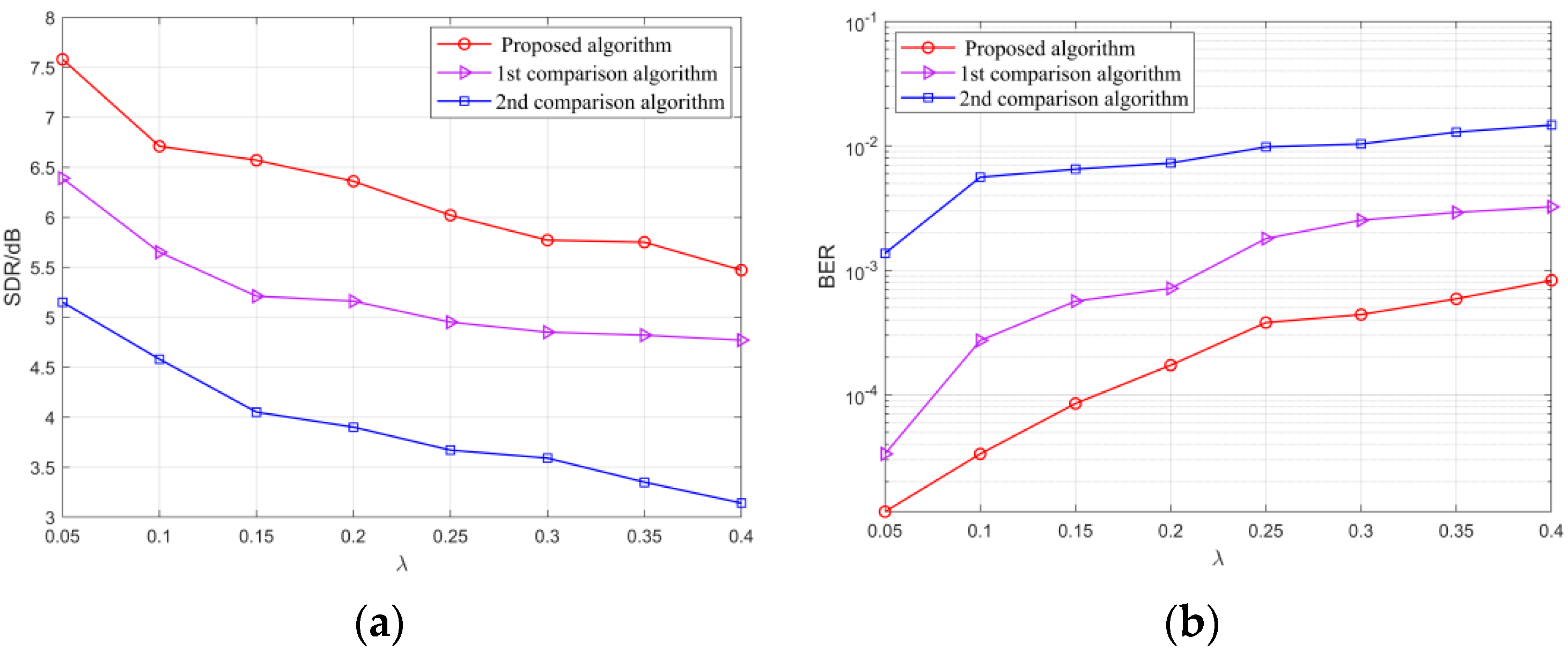
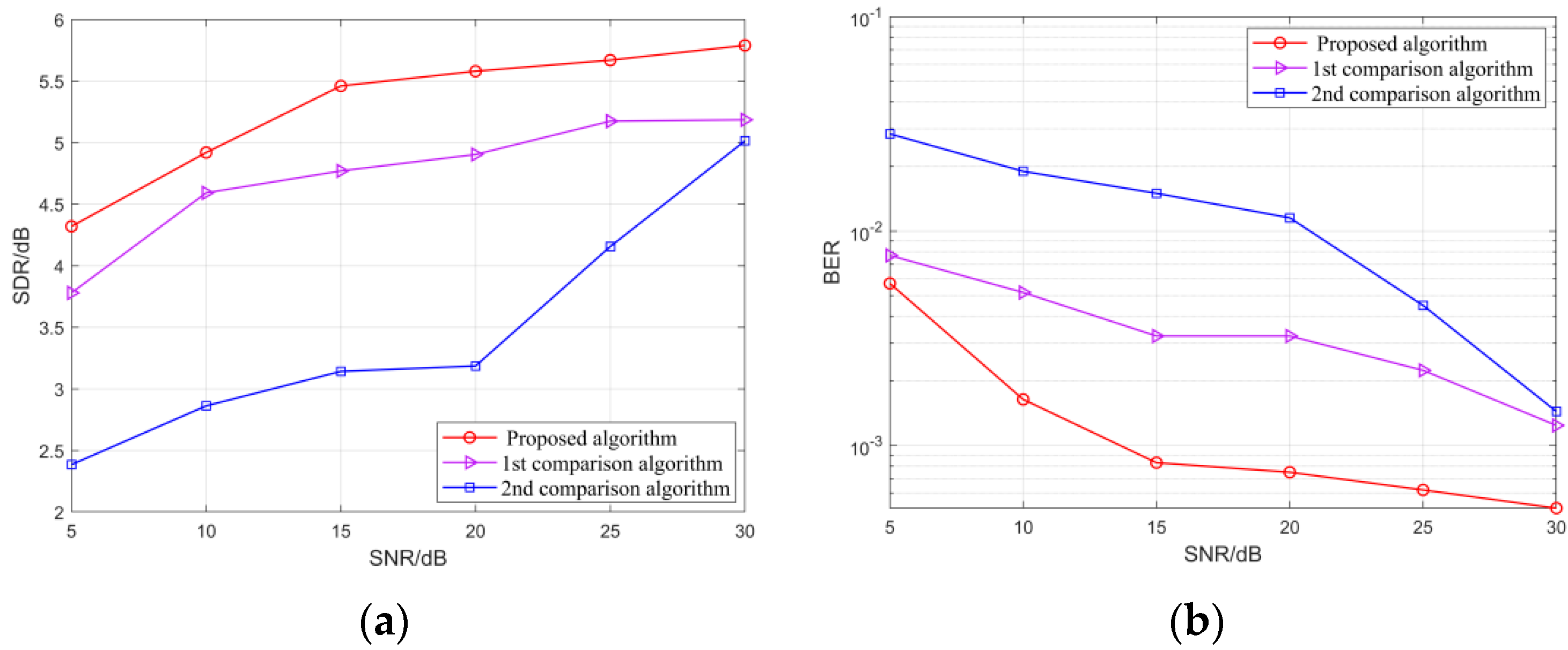
4.3. Simulation 3: Simulation of Algorithm Anti-Noise Performance

In this simulation, the carrier frequency of each of the two groups of source signals was set to 14 MHz, 20 MHz, and 26 MHz, and the λ was fixed at 40% correspondingly. In the environment of the SNR from 5 to 30 dB, the method in simulation two was used to mix the source signals. The SDR and BER of the separated signals with the increase in the SNR are shown in Figure 15 and Figure 16:
It can be seen from Figure 15 and Figure 16 that, with the SNR increases, the separation performance of the algorithm proposed in this paper and the comparison algorithms have been effectively improved. However, compared with the comparison algorithms, the SDR and BER of the separated signals by the proposed algorithm are higher and lower, respectively, indicating that the signal separation performance is better. Especially for signals with the same BPSK modulation (Figure 15), when the SNR is 10, the BER of the separated signals is lower than 102. For signals with different modulation (Figure 16), the BER drops below 102 when the SNR reaches 20 dB.

5. Conclusions

In this paper, we have discussed an underdetermined mixed blind signal separation method with the application of TF overlapped communication signals. The classical SCA methods to solve the UBSS problem require high sparsity of the signal. For TF overlapped signals, the classical SCA methods cannot be applied to such problems. To tackle this issue, we propose a novel method for separating TF overlapped signals based on the SCA algorithm. The core idea of the method is to construct a reasonable TF soft mask matrix by designing a contribution degree function. In the proposed method, we utilize the KDE algorithm to obtain the angle probability density distribution, followed by which the source number is estimated by detecting the peak points of the distribution. Then the contribution degree function is designed to generate the contribution degree, based on which the TF soft mask matrix is constructed to obtain the reconstructed TF signal. The sparsity requirement of the algorithm is reduced by constructing a reasonable TF soft mask matrix, which makes the separation algorithm suitable for separating TF overlapped signals. Compared with the classical SCA algorithm, the most significant contribution of the proposed algorithm is to expand the application scope of the SCA algorithm, which no longer requires the signal to have sparsity in the TF domain. In addition, the source estimation process prior to separation enables it to adapt to the case in which the number of sources is unknown. The algorithm’s anti-aliasing ability and anti-noise ability are simulated and verified by simulation, which demonstrates that the proposed method enables to overcome the poor performance of blind separation for TF aliasing communication signals by classical separation algorithms.

Author Contributions

Conceptualization, H.M. and X.Z.; methodology, H.M. and X.Z.; writing—original draft preparation, H.M.; writing—review and editing, X.Z., L.Y., X.W. and Y.Z. All authors have read and agreed to the published version of the manuscript.

Funding

This research did not receive any specific grant from funding agencies in the public, commercial, or not-for-profit sectors.

Institutional Review Board Statement

Not applicable.

Informed Consent Statement

Not applicable.

Data Availability Statement

Data sharing not applicable to this article as no datasets were generated or analyzed during the current study.

Acknowledgments

The authors would like to thank the anonymous reviewers and the editors for helping improve this work.

Conflicts of Interest

The authors declare no conflict of interest.

Abbreviations

TFTime–frequency
KDEKernel density estimation
BSSBlind source separation
ICAIndependent component analysis
UBSSUnderdetermined blind source separation
SCASparse component analysis
RFRadio frequency
STFTShort-time Fourier transform
SSPSingle-source-point
ISTFTInverse short-time Fourier transform
SDRSource-to-distortion ratio
SIRSource-to-interferences ratio
SARSource-to-artifacts ratio
BERBit error rate
SNRSignal-to-noise ratio

References

  1. Wei, C.; Hua, P.; Junhui, F. A Blind Separation Method of PCMA Signals Based on MSGibbs Algorithm. J. Phys. Conf. Ser. 2019, 1168, 052050. [Google Scholar]
  2. Miao, W.; Xiao-xia, C.; Ke-fan, Z. A Blind Separation of Variable Speed Frequency Hopping Signals based on Independent Component Analysis. In Proceedings of the 2019 IEEE 3rd Information Technology, Networking, Electronic and Automation Control Conference (ITNEC), Chengdu, China, 15–17 March 2019; pp. 144–148. [Google Scholar] [CrossRef]
  3. Sharma, R. Musical Instrument Sound Signal Separation from Mixture using DWT and Fast ICA Based Algorithm in Noisy Environment. Mater. Today Proc. 2020, 29, 536–547. [Google Scholar] [CrossRef]
  4. Ziani, S.; Jbari, A.; Bellarbi, L.; Farhaoui, Y. Blind maternal-fetal ECG separation based on the time-scale image TSI and SVD–ICA methods. Procedia Comput. Sci. 2018, 134, 322–327. [Google Scholar] [CrossRef]
  5. Luo, Z.; Li, C.; Zhu, L. A comprehensive survey on blind source separation for wireless adaptive processing: Principles, perspectives, challenges and new research directions. IEEE Access 2018, 6, 66685–66708. [Google Scholar] [CrossRef]
  6. Ma, B.; Zhang, T. Single-channel blind source separation for vibration signals based on TVF-EMD and improved SCA. IET Signal Process. 2020, 14, 259–268. [Google Scholar] [CrossRef]
  7. Zhen, L.; Peng, D.; Yi, Z.; Xiang, Y.; Chen, P. Underdetermined blind source separation using sparse coding. IEEE Trans. Neural Netw. Learn. Syst. 2016, 28, 3102–3108. [Google Scholar] [CrossRef] [PubMed]
  8. Fang, B.; Huang, G.; Gao, J. Underdetermined blind source separation for LFM radar signal based on compressive sensing. In Proceedings of the 2013 25th Chinese Control and Decision Conference (CCDC), Guiyang, China, 25–27 May 2013; pp. 1878–1882. [Google Scholar]
  9. Fu, W.; Chen, J.; Yang, B. Source recovery of underdetermined blind source separation based on SCMP algorithm. IET Signal Process. 2014, 11, 877–883. [Google Scholar] [CrossRef]
  10. Yu, G. An Underdetermined Blind Source Separation Method with Application to Modal Identification. Shock. Vib. 2019, 2019, 1637163. [Google Scholar] [CrossRef]
  11. Cobos, M.; Lopez, J.J. Maximum a posteriori binary mask estimation for underdetermined source separation using smoothed posteriors. IEEE Trans. Audio Speech Lang. Process. 2012, 20, 2059–2064. [Google Scholar] [CrossRef]
  12. Kumar, M.; Jayanthi, V.E. Underdetermined blind source separation using CapsNet. Soft Comput. 2020, 24, 9011–9019. [Google Scholar] [CrossRef]
  13. Li, Y.; Nie, W.; Ye, F.; Lin, Y. A mixing matrix estimation algorithm for underdetermined blind source separation. Circuits Syst. Signal Process. 2016, 35, 3367–3379. [Google Scholar] [CrossRef]
  14. Liu, Z.; Li, L.; Lv, D.; Pan, N. Novel source recovery method of underdetermined time-frequency overlapped signals based on submatrix transformation and multi-source point compensation. IEEE Access 2019, 7, 29610–29622. [Google Scholar] [CrossRef]
  15. Reju, V.G.; Koh, S.N.; Soon, I.Y. Underdetermined convolutive blind source separation via time-frequency masking. IEEE Trans. Audio Speech Lang. Process. 2009, 18, 101–116. [Google Scholar] [CrossRef]
  16. Reddy, A.M.; Raj, B. Soft mask methods for single-channel speaker separation. IEEE Trans. Audio Speech Lang. Process. 2007, 15, 1766–1776. [Google Scholar] [CrossRef]
  17. Duan, T.; Zhang, X. A solution to blind separation of convolutive communication mixtures in frequency domain. In Proceedings of the 2012 2nd International Conference on Consumer Electronics, Communications and Networks (CECNet), Yichang, China, 21–23 April 2012; pp. 2330–2333. [Google Scholar]
  18. Ma, B.; Zhang, T.; An, Z.; Song, T.; Zhao, H. A blind source separation method for time-delayed mixtures in underdetermined case and its application in modal identification. Digit. Signal Process. 2021, 112, 103007. [Google Scholar] [CrossRef]
  19. Li, C.; Zhu, L.; Luo, Z. Underdetermined blind source separation of adjacent satellite interference based on sparseness. China Commun. 2017, 14, 140–149. [Google Scholar] [CrossRef]
  20. Lu, J.; Cheng, W.; He, D.; Zi, Y. A novel underdetermined blind source separation method with noise and unknown source number. J. Sound Vib. 2019, 457, 67–91. [Google Scholar] [CrossRef]
  21. Özbek, M.E. Determining the Number of Sources with Diagonal Unloading in Single-Channel Mixtures. Circuits Syst. Signal Process. 2021, 40, 5483–5499. [Google Scholar] [CrossRef]
  22. Węglarczyk, S. Kernel density estimation and its application. ITM Web Conf. 2018, 23, 00037. [Google Scholar] [CrossRef]
  23. Vincent, E.; Gribonval, R.; Fevotte, C. Performance measurement in blind audio source separation. IEEE Trans. Audio Speech Lang. Process. 2006, 14, 1462–1469. [Google Scholar] [CrossRef] [Green Version]
Figure 1. The power scatters of mixed signals without TF aliasing.
Applsci 12 06534 g001
Figure 2. The power scatters of mixed signals with TF aliasing.
Applsci 12 06534 g002
Figure 3. The statistical histogram of angular distribution.
Applsci 12 06534 g003
Figure 4. The angular probability density distribution.
Applsci 12 06534 g004
Figure 5. The sum of the power data.
Applsci 12 06534 g005
Figure 6. The power scatters of mixed signals after detection.
Applsci 12 06534 g006
Figure 7. The flowchart of the proposed method.
Applsci 12 06534 g007
Figure 8. The separation performance with different γ .
Applsci 12 06534 g008
Figure 9. The waveforms of source signals.
Applsci 12 06534 g009
Figure 10. The waveforms of mixed signals.
Applsci 12 06534 g010
Figure 11. The waveforms of separated signals.
Applsci 12 06534 g011
Figure 12. The waveforms of separated signals after coherent demodulation.
Applsci 12 06534 g012
Figure 13. (a) The SDR of three BPSK signals with different λ ; (b) The BER of three BPSK signals with different λ . The 1st and 2nd comparison algorithms are given in literatures [8,10], respectively.
Applsci 12 06534 g013
Figure 14. (a) The SDR of different modulation signals with different λ ; (b) The BER of different modulation signals with different λ . The 1st and 2nd comparison algorithms are given in literatures [8,10], respectively.
Applsci 12 06534 g014
Figure 15. (a) The SDR of three BPSK signals under different SNR; (b) The BER of three BPSK signals under different SNR. The 1st and 2nd comparison algorithms are given in literatures [8,10], respectively.
Applsci 12 06534 g015
Figure 16. (a) The SDR of different modulation signals under different SNR; (b) The BER of different modulation signals under different SNR. The 1st and 2nd comparison algorithms are given in literatures [8,10], respectively.
Applsci 12 06534 g016
Table 1. Variable definitions involved in the problem statement.
VariableMeaning
s ( t ) The source signal.
x ( t ) The received signal.
A q The mixing matrix corresponding to the qth wireless propagation path of the signal.
a k i q The amplitude attenuation of the ith source signal to the kth sensor through the qth path.
τ k i q The time delay of the ith source signal to the kth sensor through the qth path.
X k ( t , f ) The STFT of the signal x k ( t ) received by the kth sensor.
P k ( f ) The power of the kth received signal.
Table 2. Variable definitions in this section.
VariableMeaning
FThe set of frequencies after removing the low power points.
θ The angular distribution.
G κ ( θ ) The angular probability density distribution of θ .
Y i ( t , f ) The STFT of the ith signal to be reconstructed.
M i ( t , f ) The corresponding ith TF soft mask matrix that needs to be constructed.
η u i The contribution degree of the ith source signal to the mixed signal.
d u i The corresponding cosine distance between the power point and the ith endpoint.
y i ( t ) The ith source signal to be reconstructed.
Publisher’s Note: MDPI stays neutral with regard to jurisdictional claims in published maps and institutional affiliations.

