Development of a CFD-Suitable Deep Neural Network Model for Laminar Burning Velocity

Featured Application

The presented DNN model has been developed for application in the CFD simulations requiring a simplified estimation of laminar burning velocity in dry hydrogen–air mixtures. A pair of examples using the progress variable approach, turbulent flame speed closure model and open-source CFD solver flameFoam are presented at the end of the paper.

Abstract

Hydrogen is a valued resource for today’s industry. As a fuel, it produces large amounts of energy and creates water during the process, unlike most other polluting energy sources. However, the safe use of hydrogen requires reliable tools able to accurately predict combustion. This study presents the implementation of a deep neural network of laminar burning velocity of hydrogen into an open-source CFD solver flameFoam. DNN was developed based on a previously created larger DNN, which was too large for CFD applications since the calculations took around 40 times longer compared to the Malet correlation. Therefore, based on the original model, a faster, but still accurate, DNN was developed and implemented into flameFoam starting with version 0.10. The paper presents the adaptation of the original DNN into a CFD-applicable version and the initial test results of the CFD–DNN simulation.

1. Introduction

The first concepts of non-biological brains were analyzed during World War II by McCulloch and Pitts [1]. Since then, multilayer deep neural networks (DNNs) have been widely used for numerous research and practical applications. In machine learning, the algorithm learns from the data, using various transformations of inputs, without a user or programmer giving it explicit instructions [2]. Various other machine learning (ML) algorithms can also be used as a replacement for neural networks since studies show that the performance of all ML algorithms depends greatly on the problem itself [3,4]. In general, an artificial neural network (ANN) performs better in finding complex behavior and patterns in large amounts of data. As stated by studies, multi-layer ANNs, such as deep neural networks (DNN) can reproduce any function with arbitrary precision [5,6].

Simulation of turbulent premixed combustion is challenging numerically due to the wide range of spatial and temporal scales involved in turbulence and combustion chemistry. Therefore, to perform practically relevant simulations, various simplified modeling approaches are usually employed, e.g., RANS treatment of turbulence or simplified combustion rate estimations instead of direct modeling of chemical kinetics. The most common approach to avoid chemical simulation is to formulate a used combustion model in a way that chemistry would be replaced by a simpler estimation of laminar burning velocity (LBV), e.g., from the correlations based on the experiments.

There are several examples of ANN and other ML methods for the application in the prediction of combustible mixture properties in the literature. In 2018, Jach et al. [7] created three ML models—ANN, SVM and multivariable regression (MR)—for LBVs of mixtures of air with one of seven hydrocarbons from methane up to n-heptane. The best performance was obtained by ANN model in terms of R², RMSE and MAE.

In 2019, Mehra et al. [8] were able to create DNN which could predict laminar burning velocities of HyCONG gas blends with an R-squared value approximately equal to 0.999 and a number of neurons up to 20. Concentrations of blend constituents were used as inputs. Authors showed that an increase in network weight number decreased the testing error, which means that DNN with more weights should have higher accuracy. Similar behavior was noticed for the number of epochs used for model optimization. However, while more complex networks can show better results, they also are slower and have a higher risk of overfitting.

In 2020, Pulga et al. [9] developed methodology to improve the accuracy of laminar flame ML simulations, starting from data preparation, model creation and finishing with model evaluation and results interpretation. Malik et al. presented a light neural network (as it only had up to five neurons in each layer), which could get good predictions in a short amount of time [10]. Their neural network could be used in real-time and had the mean squared error equal to 0.3023 (m/s)² with hydrogen–air mixtures for laminar burning velocity predictions. In their work, 577 observations were used for the training of DNN. Part of them had a high spread and this can lower prediction accuracy. Since the amount of available experimental data was insufficient to train the neural network, the study generated new points (up to 7300 observations) for training. Varghese and Kumar [11] analyzed syngas mixtures and created multiple linear regression model to predict their LBVs with error <10%. Their model was derived partly from the measured velocities, and partly from the predictions using FFCM-1 kinetic mechanism.

In 2021, Eckart et al. [12] compared four different machine learning algorithms predicting laminar burning velocities of hydrogen–methane mixtures. Their study showed that the DNN model can give much better predictions than other popular algorithms such as support vector machines (SVM) or random forest while predicting velocities for hydrogen–methane mixtures. Correa et al. [13] used several ML methods to predict the research octane numbers of several spark ignition fuels. Study evaluated multiple ML algorithms using 10-fold cross validation, which ensured that results are less influenced by noise and more accurately reflects real capabilities of these models. In this study SVM gave best predictions out of all tested methods. vom Lehn et al. [14] created a quantitative structure–property relationship (QSPR) model for the estimation of LBVs of hydrocarbons and oxygenated hydrocarbons based on their underlying fuel structures. A set of molecular groups as well as pressure, temperature and equivalence ratio served as input parameters to an ANN, which has been trained based on a large database of training data for 124 different compounds.

Recently, Wan et al. [15] compared 16 ML algorithms for the prediction of hydrocarbon and oxygenated fuels LBVs and found out that the Gaussian or Tree-based methods gave high predictions with most of those models explaining over 90% of all data. Li et al. [16] created ML–QSPR model to screen fuels based on their predicted properties.

In our previous work [17], we created a DNN for the prediction of the laminar burning velocity of hydrogen–air mixtures with a coefficient of determination approximately equal to 0.985. However, this model was too slow to be used practically (in CFD calculations)—the testing script could make a million predictions in around 45 s, compared to the Malet correlation [18], with which predictions could be made under the same conditions in less than a second.

For complex combustion cases, increases in observation quantity can highly improve predictions of neural networks. However, as the network starts to learn the way to solve the problem, this effect gets less visible. In the end, if the model overlearns on data, it can even start to mimic the noise. Therefore, the goal should be to obtain a high enough amount of well-balanced data. Since there are more data in the specific region, the more trustworthy prediction can be made by the neural network.

To achieve more accurate predictions, aberrant outliers may need to be removed from the data. As suggested by J. Heaton, this can be carried out with the so-called ‘double-D’ algorithm [19]. The algorithm itself has many names, however, the idea behind it is to use a double standard deviation as a removal condition. However, it is more useful when the database has a very large number of observations. Since the amount of experimental data on hydrogen–air LBV in the literature is not that large, this method might not significantly improve predictions as the neural network might not have enough data to learn well. On the other hand, it could be a direction for future work. Moreover, outliers have a significant influence on the mean value as it is one of the neural network’s measures based on which it decides how the final model will look like. Luckily, the model can also be evaluated using mean absolute error (MAE) instead. The influence on a model based on MAE compared to a model based on mean squared error (MSE) was analyzed by J. Qi [20]. It is much less affected by outliers but error can be influenced by the number of observations. As pointed out by T. Chai [21], each metric has its advantages and disadvantages. Due to this, it would be wise to have the MSE as a side evaluator as well and not trust in a single measure (MAE) blindly.

As the presented research overview shows, most of the related studies to date have focused on the development of stand-alone ML models of combustible mixtures’ properties. While there are works considering the implementation of such a model into a CFD code [10], this has not been performed up to now. Consequentially, when developing, there is less pressure to create lean and fast, but sufficiently accurate models, and their suitability is not tested in CFD frameworks. In addition, the last, but main step, producing a working, research or application suitable CFD–ANN code is never performed. To fill this gap, we have developed a CFD-suitable deep neural network model for hydrogen LBV and implemented it into an actual OpenFOAM-based CFD solver flameFoam.

The purpose of the current paper is to, based on the literature and our previous work [17], create a fast and light, suitable for CFD applications, DNN model for LBV in dry hydrogen–air mixtures, implement the developed model into a CFD solver, and perform testing CFD–DNN simulations of turbulent premixed combustion.

2. Developed Deep Neural Network Model for Laminar Burning Velocity

The presented model was based on a previously developed (further referred to as the original) large DNN [17], which was too slow for CFD application. The further model development aimed to improve the calculation speed without a significant accuracy loss. The original DNN model was trained on the dataset of experimental hydrogen–air mixtures LBV at various temperatures, pressures and hydrogen concentrations, collected from the open literature [17].

For the training of the new DNN model, the original database was expanded to 2871 data points [22,23,24,25,26,27,28,29,30,31,32,33,34,35,36,37,38,39,40,41,42,43,44,45,46,47]. Around 33% of all of them are experimental values; however, the number of pure experimental values was insufficient for the reliable training of DNN. Therefore, additional values were interpolated from the experimental values, by adding points from the correlation curve produced from the experimental points of the given experiment, close to the actual experimental points. Since the results of the newest studies are most likely to have a higher accuracy due to technological development, they were prioritized for the interpolation, in this way giving them more ‘weight’ in the final database, since more data points have been added based on the newest observations and fewer points in the area near old observations.

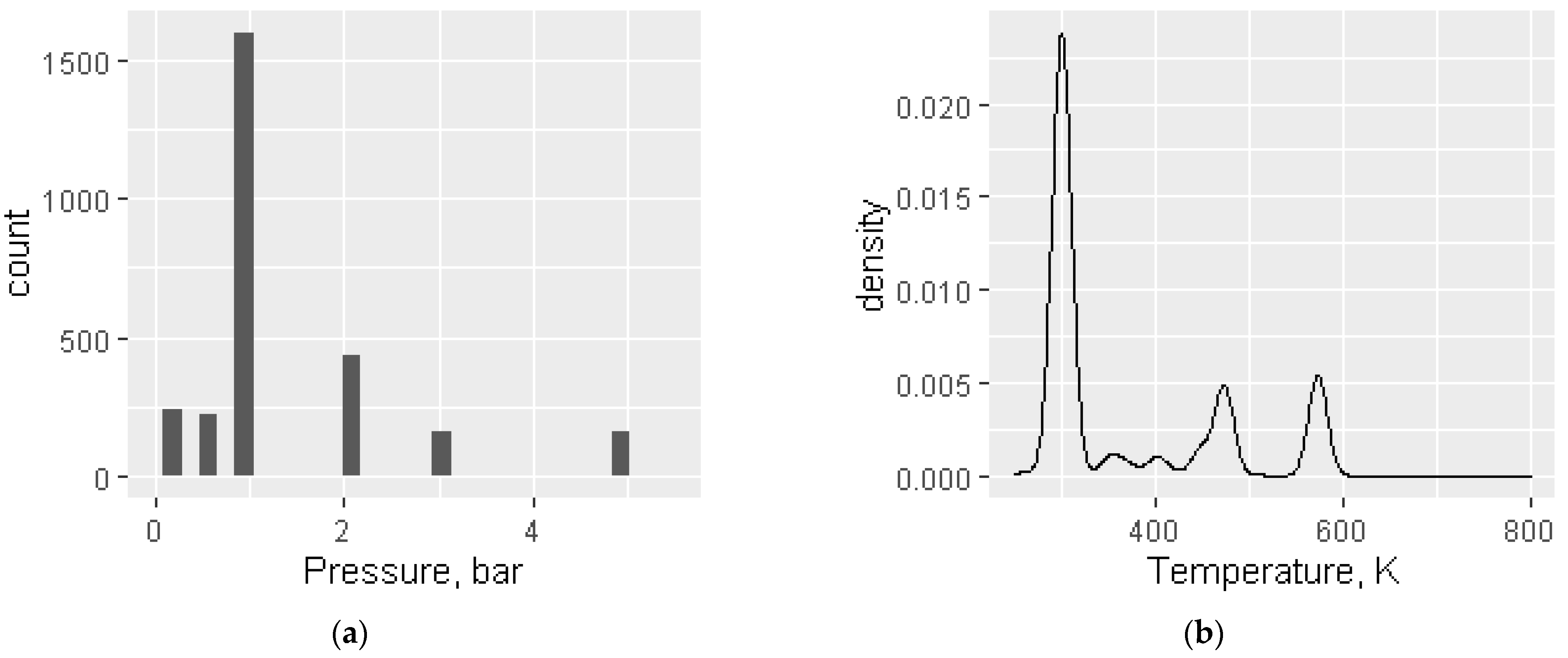
As can be noticed from Figure 1, most of the data are around 1 bar pressure or 298 K temperature, because most experimental works start by taking normal conditions and changing only a single parameter. However, the expansion of the database was performed to make the model more reliable while predicting LBVs at higher temperatures and higher pressures, since most of the new data are under non-normal conditions. These changes should have made the model more reliable in an entire applicability range. The used experimental data model is applicable in the range of 295–600 K temperature and 0.1–5 bar pressure.

Data were split randomly into training and testing sets with around 75% of data used to train the model and the remaining data used for validation. Further modifications such as outlier removal were focused on the training set, avoiding modification of the testing set, this way trying to obtain as reliable data as possible for validation.

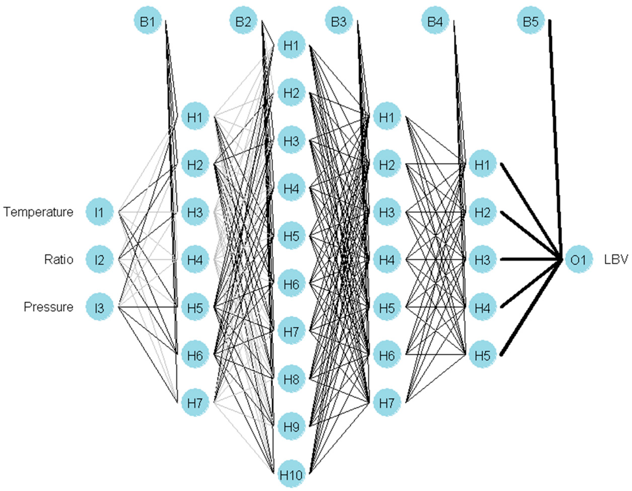
Four hidden layers were left in the new model (same as in the original); however, to ensure faster calculations, the number of neurons was changed to (7,10,7,5) (Figure 2) from (40,50,30,10) in previous work [17]. The number of neurons was reduced by trying various combinations and balancing accuracy against prediction speed.

In general, reducing the number of neurons increased the risk that the model will not be as robust to data as the previous model. Due to this, we had to re-train the model multiple times as changes in weights could affect the predictions. Overall, this meant that the smaller neural network required more human monitoring during the training to lessen accuracy loss. In addition, we increased the risk that fewer neurons will lack data to learn in some areas; to counter this, we had to increase our database. In the end, the main drawback related to the reduced number of neurons was that we had to put in substantial additional effort to obtain the model with results comparable to those of larger DNN.

Several different sets of activation functions were also tested and the best predictions were obtained when using tanh activation function for the first (dense) hidden layer (Equation (1)) and ReLU for the rest (Equation (2)):

$$tanh\left(z\right)\frac{e^z-e^{-z}}{e^z+e^{-z}}$$

(1)

$$ReLU\left(output\right)=\{\begin{array}{c}output,ifoutput>0;\\ 0,else\end{array}$$

(2)

The original model used only ReLU functions [18]; however, the switch to tanh function in the first layer gave accuracy improvement to the new model. Further inclusions of tanh functions did not produce significant further improvement, even though in the literature there is an example of LBV–DNN with all tanh activation functions [11]. Since tanh function takes longer to calculate and did not give a significant advantage when used in deeper layers, we left the ReLU activation function in those layers. Result improvement might have been achieved since the tanh activation function managed to give primary predictions which later were adjusted by layers with ReLU bending curve so that it would fit data better.

However, since the number of neurons is not large, it is likely that with small laminar burning velocities (0 m/s or close to it), the model might predict values below zero. To avoid negative predictions, the Equation (2) was also applied to the final output function.

For model optimization RMSprop optimizer was used [48]. As studies show, it is one of the best methods for optimization [49]. In addition, the regularization parameters were changed compared to the original model. The first layer had Ridge (L2) regularization parameter equal to 0.000002 and other hidden layers had Lasso (L1) regularization equal to 0.0004. These values were selected after multiple tests with varied values. The effects of the decrease in errors due to L1 and L2 are well documented in [50,51]. In general, they prevent DNN from overfitting, which makes the network more stable and reliable.

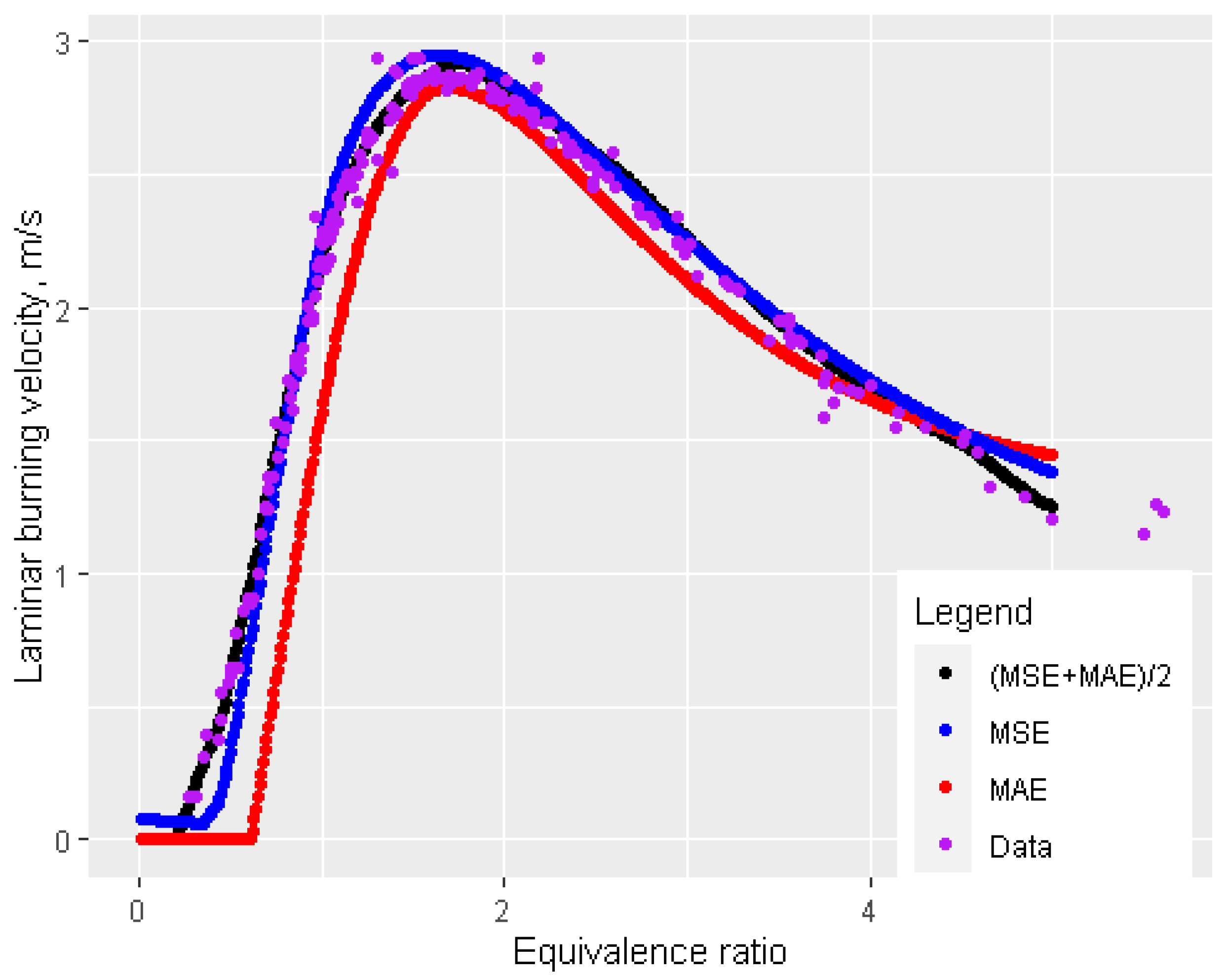
To improve the reliability of the new model, MAE and MSE errors were combined and minimized as weighted errors (equal weights were selected after several test cases) for the training of the model as a loss function. Most of the influence was displayed by MAE since velocity was in meters per second and lower than 1 m/s. On the other hand, MSE helped in cases when MAE became almost constant. We believe this approach could give predictions closer to real values, as performed analysis shows that averaging MAE and MSE indeed gives values in between for the data gathered for this research. This can be helpful in cases with areas lacking observations. Also, it is worth noticing that in cases of unique (single) observations, the MAE and MSE will point to the same location. A simple explanation of this could be the idea that while MAE minimizes the model towards median and MSE—towards mean, the combination of them would predict the value in between as visualized in Figure 3.

To obtain predictions closer to original experimental values, the study did not modify the testing set; however, the training set for improved DNN was adjusted by making some outliers equal to the mean. Outliers were considered values that are different by over 10% from the median value when results from three or more different experimental sources under the same or similar conditions were available. These values were considered outliers since the experimental spread of more than 10% shows higher experimental uncertainties, and given several sources, aberrant points are the most suspect. Around 3–4% of all points were adjusted. Yet, considering that this can detect many data points near zero, those values were ignored. Due to the way in how the model was trained, outliers still could have influenced the final model. However, due to the mean value, this influence is reduced. This allowed the creation of a model which is stable and can perform well on data sets that have outliers.

To use this model in the CFD solver, it was exported by saving the weights $w_{i_{j-1},i_j,j}$, biases b_i,j and performing matrix multiplication with them. Here, j denotes a layer number, and i_j denotes a weight number in the j-th layer. j can obtain values from 1 to k and i_j can obtain values from 1 to n_j. Then the i-th value in the j-th hidden layer h_i,j is obtained from the Equations (3) and (4):

$$h_{i,j}^{*}=w_{i,0,j}{h}_{0,j-1}+w_{i,1,j}{h}_{1,j-1}+\dots +w_{i,n_{j-1},j}{h}_{n_{j-1},j-1}$$

(3)

$$h_{i,j}=actF\left(h_{i,j}^{*}+b_{i,j}\right),$$

(4)

where actF is an activation function given by the Equations (1) and (2) for the first and other layers, respectively. By applying Equations (3) and (4), the model can be expressed and implemented using weights (W_j) and biases (B_j) matrixes and inputs vector (I). Weights and biases can also be expressed as follows by Equations (5) and (6) in which n and k mark the number of weights in interacting layers.

$$W_j=\left[\begin{array}{ccc}{w}_{1,1}& \dots & w_{n_j,1}\\ \dots & \dots & \dots \\ w_{1,n_{j-1}}& \dots & w_{n_j,n_{j-1}}\end{array}\right]$$

(5)

$$B_j=\left(b_1,..,b_{n_j}\right)$$

(6)

The output becomes the new input for the next layer. This process is repeated until all layers are calculated and the final output—value of LBV is predicted.

3. Comparison with Other Methods

To test the quality of the developed DNN model and to check whether some simpler method could be sufficient, other models using popular machine learning methods were created based on the same database. All models were optimized to make a million predictions in under 2 s with a testing script. Final models were tested and compared with DNN in terms of prediction density and the most widely used metrics such as MAE, MSE and R-squared. While density estimates are not the most optimal method of comparison, we reduced the Gaussian kernel and estimation for all methods which was carried out with the same kernel; therefore, we consider it to be sufficient for comparison purposes. For all models, the same training and testing datasets were used as for the developed DNN model (75%/25%).

Density plots in Figure 4 explain the high spread (

Table 1. Comparison of machine learning algorithms (values calculated against testing set).

Model	MSE, (cm/s2)	MAE, (cm/s)	R-Squared
DNN	73.07057	6.094699	0.9972631
SVM (SVR)	843.9467	23.36927	0.9687515
Random Forest	1100.299	23.68055	0.9650517
K-Nearest Neighbors (k-NN)	1164.565	18.31963	0.9541389
MARS	1324.741	24.40525	0.9487737

) of some models (RF, MARS). While DNN and k-NN both show good agreement with the density of data until LBV reaches 350 cm/s, k-NN shows worse results at higher velocities. Even more, only SVM and DNN models predict higher than 700 cm/s laminar burning velocities. On the other hand, evaluation of SVM shows that this model is most likely to make predictions too high at over 280 cm/s and otherwise, guesses too low. As stated by this study earlier, DNN was trained by minimizing MAE and MSE at the same time, which should give optimal prediction between median and mean values. It means that the model might not have the lowest MSE and MAE values; therefore, it would be wise to evaluate it based on how well it explained the data. However, the results show (see Table 1) that DNN has the lowest MEA and MSE values of all tested methods with the highest being R-Squared at approximately 0.997. The second place would go to SVM regression which shows less spread than other models (RF, k-NN, MARS). The remaining solutions performed well by showing the ability to explain most of the data; however, their main drawback is the limited ability to predict higher burning velocities.

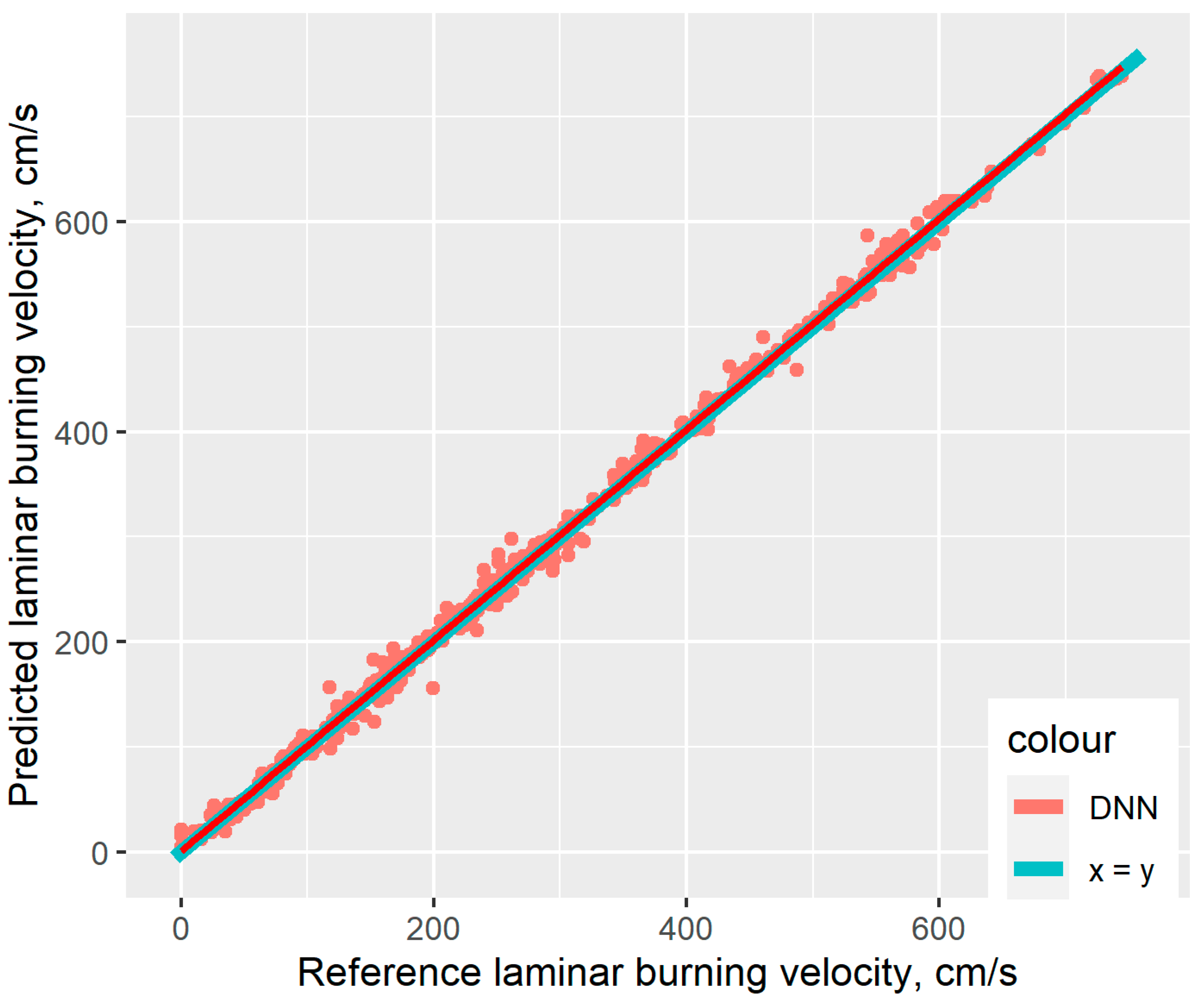
The good performance of the developed DNN model can be visible in Figure 5 below, which shows the comparison of experimental and predicted LBV values. The red line, which shows linear regression of DNN predictions plotted against reference velocities, almost perfectly covers the perfect match line (light blue).

LBV has high uncertainty in the equivalence ratio range [0.2, 0.5]. Malet [18] investigated the burning behavior of hydrogen mixtures and offered an expression to calculate LBV at low equivalence ratios. A comparison of the DNN model and Malet formula predictions (Figure 6) shows that the DNN model gives predictions closer to reality with MAE equal to 0.0589 m/s, while the Malet correlation has MAE of 0.1002 m/s.

4. CFD Simulations

This chapter presents a couple of flameFoam-DNN calculation examples showing that the developed DNN model is usable with CFD simulation and provides results in line with the Malet correlation or experimental data.

The developed model was implemented in the open-source turbulent premixed combustion solver flameFoam [52] v0.10. flameFoam is an OpenFOAM-based solver using a progress variable approach and turbulent flame speed closure model to simulate combustion. The turbulent flame speed closure model requires turbulent flame speed values, which in turn require LBV values. In the flameFoam-DNN simulations, presented below, these LBV values were estimated on-the-fly in the flameFoam using the DNN model programmed according to Equations (3)–(6) with the weights exported from the DNN training. The solver source code, including the DNN model, is available on GitHub: https://github.com/flameFoam/flameFoam (accessed on 29 June 2022).

To compare flameFoam calculation results obtained using the DNN model versus Malet correlation, simulation of ENACCEF2 facility (France, CNRS-ICARE) TEST1 from ETSON-MITHYGENE benchmark [53] was performed.

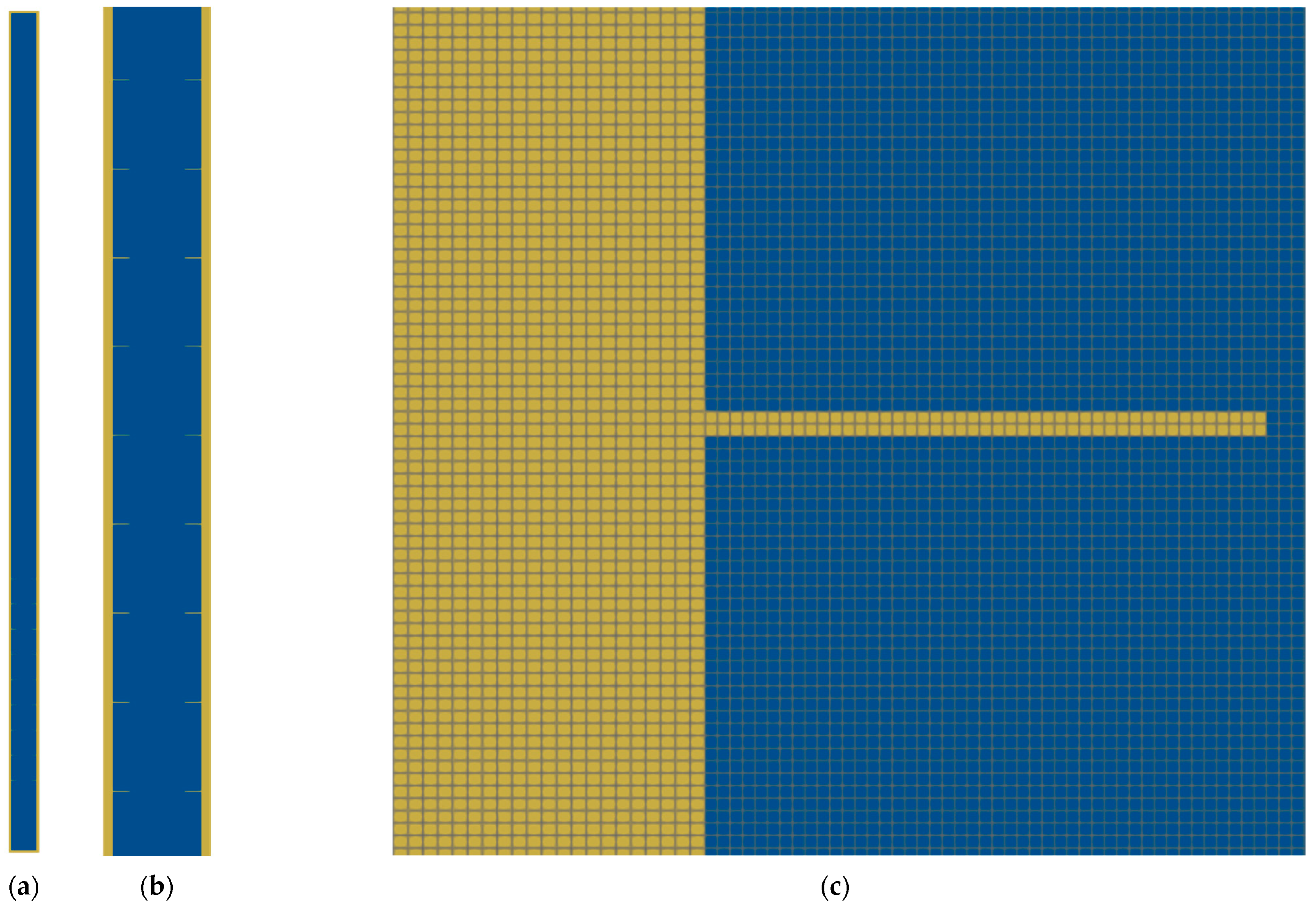
ENACCEF2 is a closed vertical steel tube of 7.65 m height and 0.23 m inner diameter (Figure 7a). Flame acceleration is achieved in the simulated experiment by 9.2 mm thin annular obstacles situated in the lower part of the facility (Figure 7b). The flame is ignited at the bottom center and propagates upwards.

The hydrogen concentration in the homogenous combustible mixture with air was 13%. The experiment was performed at 23 °C temperature and 100,000 Pa pressure.

The computational mesh (Figure 7c) of the facility was composed of the structured orthogonal grids of the facility-free volume (fluid region, blue in Figure 7) and facility wall (solid region, yellow in Figure 7). 2D axisymmetric mesh with 1 mm cell sizes was used in the presented simulations. In the fluid region, flameFoam solves Navier-Stokes, turbulence and combustion equations, while in the solid region heat conductivity equation is solved. The regions are coupled through standard OpenFOAM inter-region boundary condition for temperature compressible::turbulentTemperatureCoupledBAffleMixed.

Initial conditions were set according to the experiment. Turbulence was modeled using the k-ε RANS model. Negligible values for initial turbulence parameters were selected. The boundary condition for temperature on the external side of the solid grid was set to 23 °C.

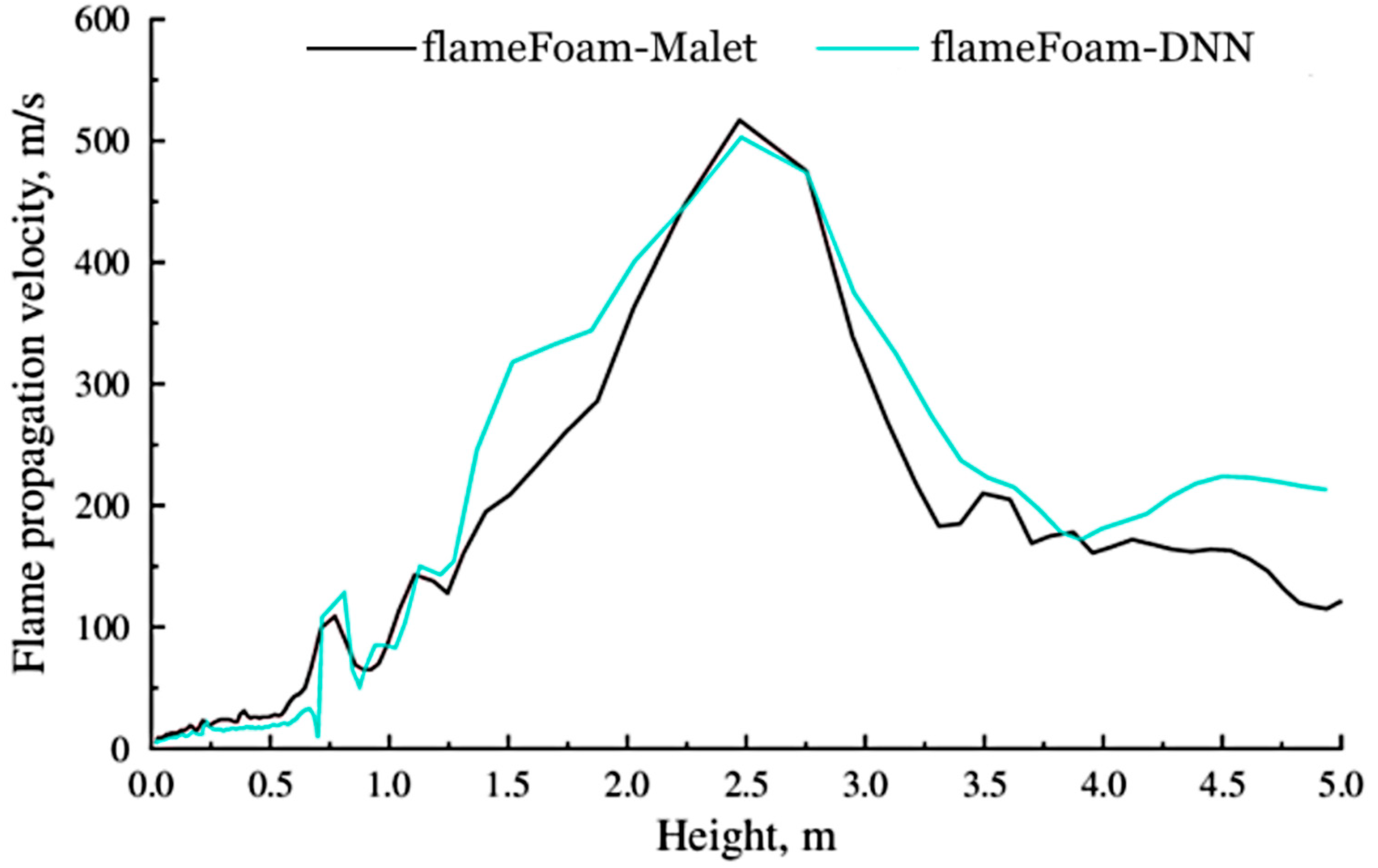
Figure 8 presents the flame propagation velocity profile (obtained from flame arrival times) obtained by both simulations. Results are very similar, showing that the DNN model hasn’t introduced any regressions compared to the Malet correlation around the experimental conditions [52]. There was no significant difference of computation time between Malet and DNN calculations.

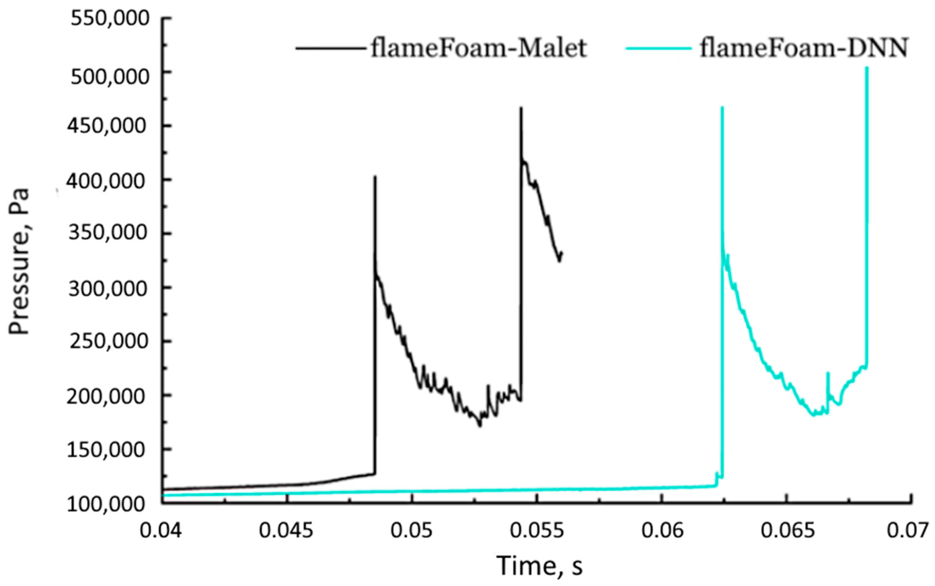
Figure 9 presents pressure evolutions at three different heights of the facility, time-shifted to facilitate comparison. Pressure evolutions corresponding to the turbulent combustion phase (accelerated flame) are also very similar in both cases. Differences between evolutions obtained with Malet and DNN seem to be mostly related to a slower (quasi-) laminar combustion phase and, consequentially, a relatively stronger impact of turbulent acceleration, which results in a higher peak pressure wave value. At a 4 m height, the peak value obtained with DNN is slightly lower; however, this seems to be a local result caused by coincidental interference, since further, at 6.2 m (Figure 10), DNN results already show higher pressure values.

Figure 10 presents pressure evolutions at a height of 6.227 m. Initial shockwave propagation and reflected shockwave arrival are visible. Results are unshifted in time to show the delay in the laminar phase simulation obtained with the DNN model compared to the Malet correlation. The DNN model provides a longer duration of quasi-laminar phase (overall slower flame propagation rate until the first obstacle). However, flameFoam with the TFC model does not simulate a quasi-laminar regime correctly [52]. The assumption is made that in turbulent cases, the main transient is controlled by the turbulent regime and the influence of the laminar phase is limited to a larger or smaller shift in time of the onset of the turbulent phase. This is partially illustrated in this case in Figure 9 and Figure 10 since different methods of laminar flame speed estimation led to different evolution and duration of the quasi-laminar regime; however, when flame accelerates due to turbulence, pressure evolutions become very similar, even including the shockwave propagation and reflection.

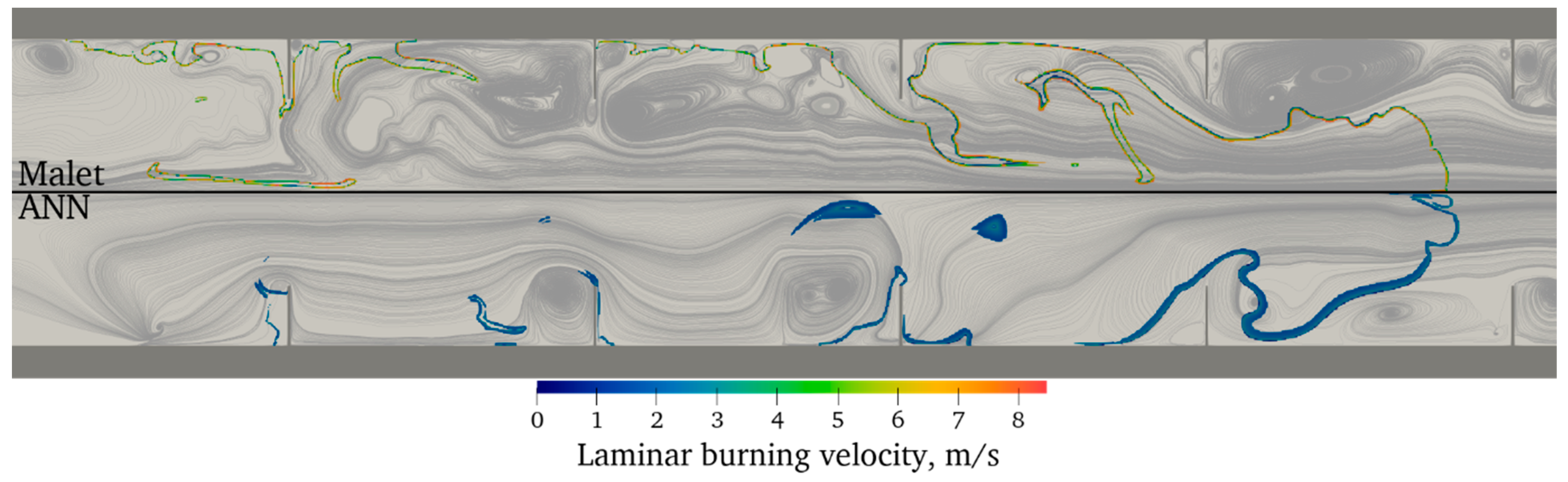
Figure 11 presents flow streamlines and laminar burning velocity values calculated in both cases when the flame is in a similar location. Only values on the flame brush (progress variable source term larger than 1000 1/s) are shown. There is a clear difference in the laminar flame velocity values obtained with both methods. The influence of pressure and temperature are far more pronounced in the Malet correlation case, where the burnt-mixture side of the flame brush exhibits two to three times higher velocity values than the leading side or whole brush in the case of the DNN model. Consequently, a very thin flame brush is obtained with Malet correlation, since combustion is completed at a higher rate. However, at the leading side of the brush, both methods seem to produce similar values of laminar burning velocity, corresponding to the similar overall flame propagation rate in both cases (Figure 8); higher values at the trailing side mostly only impact the flame brush thickness.

To validate the DNN model at a somewhat higher concentration, where the Malet correlation becomes not valid, a simulation of 22.65% hydrogen–air mixture combustion in the vented laboratory-scale chamber of the University of Sydney (US) [54] was performed.

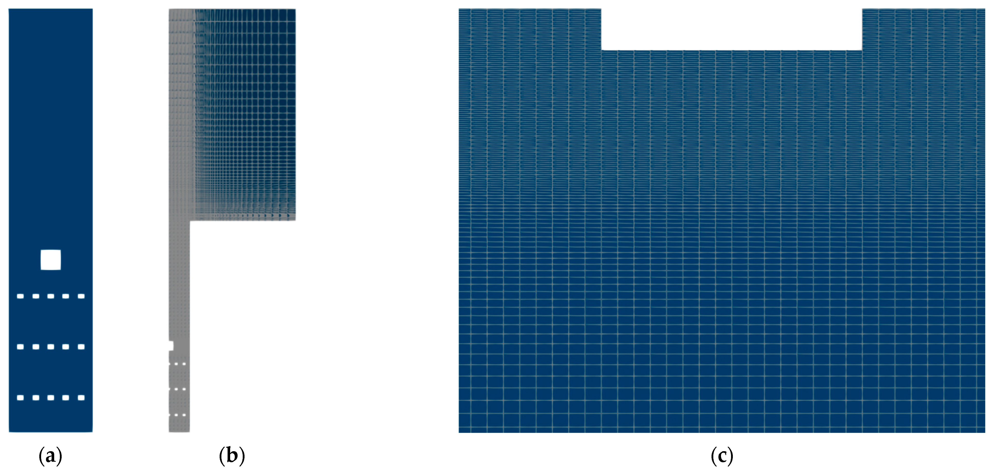
The US chamber is a rectangular box of 5 × 5 × 25 cm dimensions with an open top. Flame acceleration can be achieved with various configurations of obstacles. In the simulated experiment, three rows of baffles and a small upper obstacle were used, the so-called configuration BBBS (Figure 12a). The flame is ignited at the bottom center and propagates upwards.

The computational mesh (Figure 12b) of the facility was composed of the structured orthogonal grid of the chamber-free volume and additional volume outside the top opening to simulate surroundings. 2D axisymmetric mesh with 0.25 mm cell sizes was used in the presented simulations. Around the obstacles, the mesh was graded up to 0.03125 mm (Figure 12c).

Initial conditions were set according to the experiment—20 °C temperature and 100,000 Pa pressure. Turbulence was modeled using the k-ω-SST RANS model. Negligible values for initial turbulence parameters were selected. The adiabatic boundary condition for temperature was set.

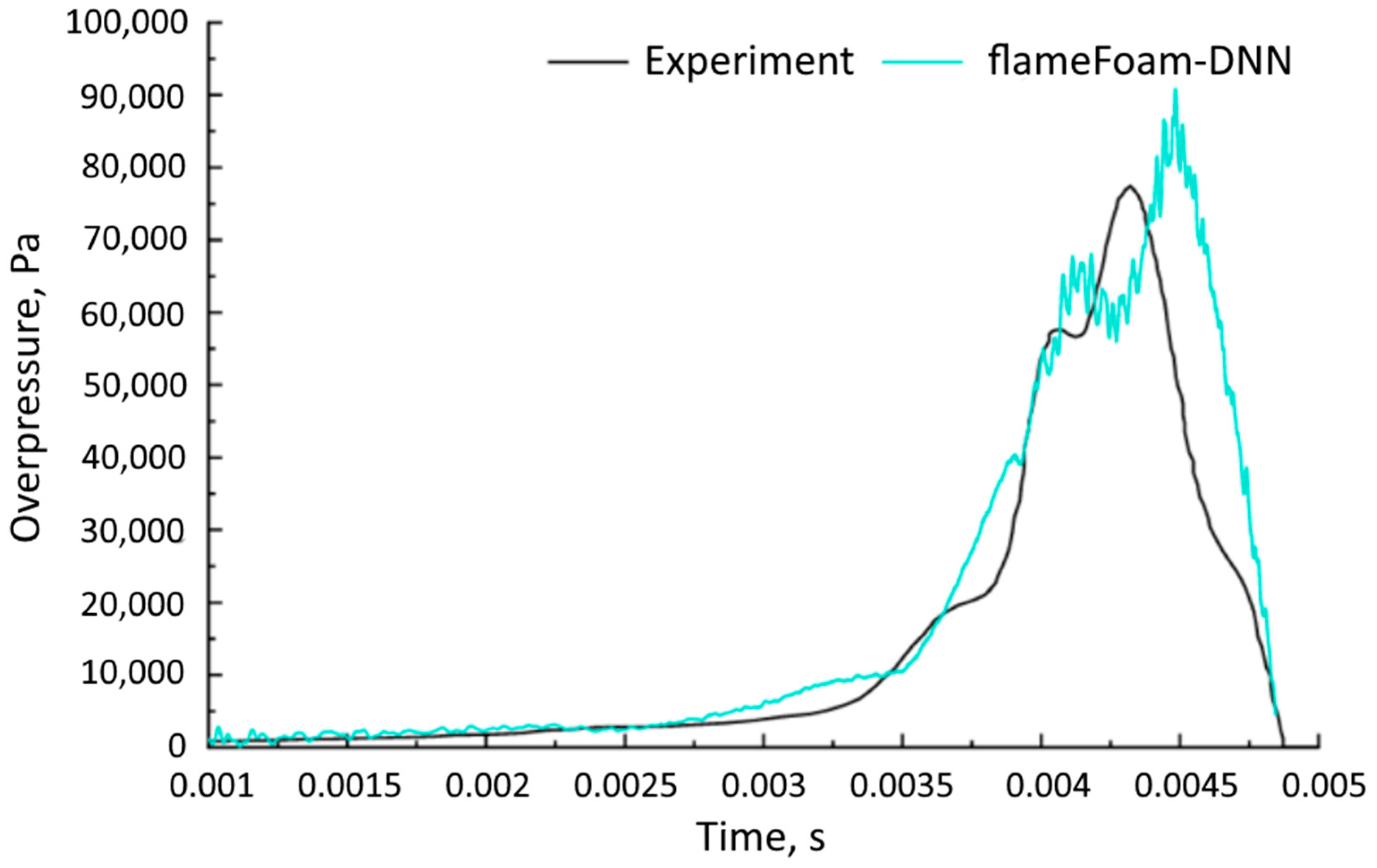
Figure 13 shows overpressure evolution at the facility’s bottom. Results obtained by flameFoam–ANN simulation are close to the experimental, including the shape of the pressure curve. However, overpressure values are slightly over-predicted. A possible explanation for the over-prediction could be missing support for quenching in the flameFoam, which, if implemented, could slightly decrease the average combustion rate in turbulent conditions and by the obstacles and wall surfaces. Nevertheless, obtained results indicate that the developed DNN model and its implementation in flameFoam are suitable for the simulation of turbulent combustion in similar conditions.

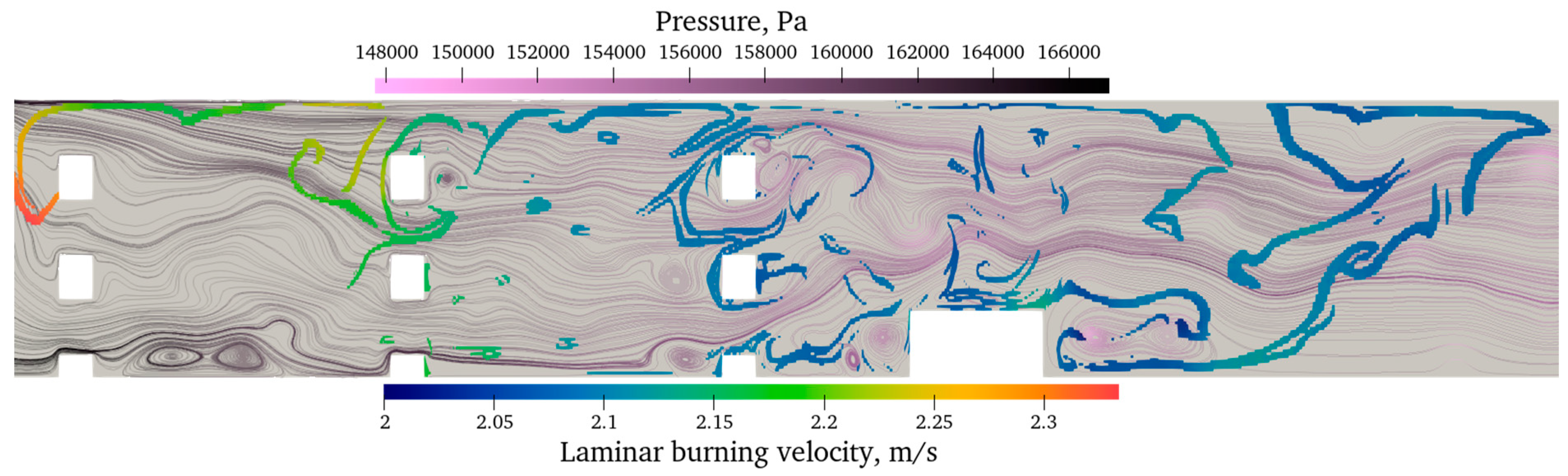
Figure 14 presents flow streamlines and laminar burning velocity values after the flame has passed the upper obstacle. Only values on the flame brush are shown. In this case, DNN–LBV predictions display similar characteristics as in the ENACCEF2 case—the predicted values do not significantly vary across the flame brush width. Obtained LBV values are not large and a thicker flame brush is also obtained. However, different LBV values are obtained in different locations of the facility, though the variation is not large. This is explained through the dependency on the pressure, which also varies in the facility as shown by the color of the streamlines. Due to venting at the facility top, there is an overall pressure gradient in the facility with the largest pressure at the bottom, and highest values reaching around 166,000 Pa. This pressure variation results in different LBV values predicted by the DNN at different heights of the facility.

5. Conclusions

A developed DNN able to predict hydrogen LBV in dry air was developed based on a larger DNN. The accuracy of fast DNN was tested against a testing set of data and values from the literature. Additionally, obtained LVB curve smoothness was checked. Predictions of developed DNN showed proper behavior and an R-squared value of approximately 0.997. Speed improvement of around 30 times compared to the original DNN was obtained.

Developed DNN was implemented into a combustion solver flameFoam for the prediction of LBV values. Testing CFD–DNN simulations were performed and compared with simulations using the established Malet correlation of LBV. The comparison showed similar results with the DNN model predicting more uniform and lower values of LBV. Comparison against a selected experiment also showed the validity of the implemented DNN model.

Further planned work is to perform validation of developed CFD–DNN modeling against the experimental data.