Article

Parallel Accelerated Fifth-Order WENO Scheme-Based Pipeline Transient Flow Solution Model

State Key Laboratory of Eco-Hydraulics in Northwest Arid Region of China, School of Water Resources and Hydropower, Xi’an University of Technology, Xi’an 710048, China
*
Author to whom correspondence should be addressed.
Appl. Sci. 2022, 12(14), 7350; https://doi.org/10.3390/app12147350
Submission received: 29 June 2022 / Revised: 13 July 2022 / Accepted: 14 July 2022 / Published: 21 July 2022
(This article belongs to the Special Issue Applied Hydrodynamics)

Abstract

:

Featured Application

Many large-scale water transmission projects, such as China’s South-to-North Water Transfer Project, are hundreds of kilometers long and need real-time regulation applications for management and control. This requires the calculation model to have higher calculation accuracy and faster calculation speed. The existing calculation models are difficult to take these two aspects into account at the same time. In this paper, the accuracy and efficiency of one-dimensional model algorithms are studied and compared, and the best calculation scheme is summarized.

Abstract

The water hammer phenomenon is the main problem in long-distance pipeline networks. The MOC (Method of characteristics) and finite difference methods lead to severe constraints on the mesh and Courant number, while the finite volume method of the second-order Godunov scheme has limited intermittent capture capability. These methods will produce severe numerical dissipation, affecting the computational efficiency at low Courant numbers. Based on the lax-Friedrichs flux splitting method, combined with the upstream and downstream virtual grid boundary conditions, this paper uses the high-precision fifth-order WENO scheme to reconstruct the interface flux and establishes a finite volume numerical model for solving the transient flow in the pipeline. The model adopts the GPU parallel acceleration technology to improve the program’s computational efficiency. The results show that the model maintains the excellent performance of intermittent excitation capture without spurious oscillations even at a low Courant number. Simultaneously, the model has a high degree of flexibility in meshing due to the high insensitivity to the Courant number. The number of grids in the model can be significantly reduced and higher computational efficiency can be obtained compared with MOC and the second-order Godunov scheme. Furthermore, this paper analyzes the acceleration effect in different grids. Accordingly, the acceleration effect of the GPU technique increases significantly with the increase in the number of computational grids. This model can support efficient and accurate fast simulation and prediction of non-constant transient processes in long-distance water pipeline systems.

1. Introduction

The water hammer pressure wave generated when a pipeline suddenly closes a valve can cause pipeline vibration, damage the valve, or cause a pipeline burst in severe cases, resulting in significant engineering accidents. Simulating, predicting, and controlling the water hammer phenomenon are critical research topics in relevant fields [1,2,3]. The commonly used solution schemes, including the MOC and the finite difference method, attempt to calculate water hammers [4,5]. The MOC requires a regular grid, while the spatial step and time step are strictly constrained by the characteristic line, limiting its applicability. Many scholars have improved the classical difference solution schemes. For example, Chaudhry and Hussaini employed the MacCormack scheme to construct an explicit finite difference scheme for solving the pipeline water hammer problem [6]. They found that the second-order finite difference scheme can achieve a computational accuracy higher than the MOC. Wan and others applied the MacCormack scheme of variable grids to transient flow simulation [7]. The mentioned scheme adopts the two-step prediction correction method to realize the flexible division of the spatial grid. Wylie and Streeter proposed an implicit finite-difference scheme for solving the water hammer problem in pipe network systems [8]. Although the main advantage of this scheme is that it remains stable for significant time steps, it requires a time-consuming iteration process. Harten proposed a scheme for solving hyperbolic partial differential equations and proved that this scheme has high resolution and no spurious oscillations at the discontinuities [4]. The finite volume method has been widely utilized in recent years for solving water hammer waves in pipelines [9]. It can provide better conservation performance and less computational time than the TVD (Total Variation Diminishing) difference scheme. Zhao and Ghidaoui constructed the first-order and second-order finite volume methods based on the Godunov scheme using the MUSCL-Hancock method to solve the water hammer problem [10]. They indicated that the second-order accuracy has better conservation at a low Courant number. Waagan proposed the prediction-correction MUSCL-Hancock finite volume method, which guarantees the accuracy of the scheme while ensuring good stability [11].
However, the second-order scheme is still limited in capturing accuracy for this aspect of strongly excited intermittent waves, and better computational results can be obtained using a higher-order scheme. The high-order ENO and WENO schemes significantly improve the capability for intermittent wave capturing [12]. The ENO scheme selects only one template among the multiple templates as the computational template, leading to inefficient computation [13]. In contrast, the WENO scheme utilizes all the templates by assigning corresponding weights to different templates through the convex combination between different templates to improve the intermittent capture performance without causing the waste of templates [14,15,16,17]. For example, Li et al. [18] obtained a new global smoothness index through the Taylor expansion of the local smoothness index. In the framework of the traditional WENO-Z format, an improved third-order finite-difference WENO format was proposed. Li et al. [19] established an improved third-order finite-difference WENO scheme based on convex combinations of different polynomials to calculate the numerical fluxes at the cell boundaries and its truncation errors and parametrization are smaller than those of other third-order WENO schemes. Moreover, the numerical results indicated that the proposed scheme performs better than other third-order WENO schemes.
To judge the performance of the model, in addition to the calculation accuracy of the model, the calculation efficiency of the model is also crucial. If the computational efficiency of the numerical scheme is too low, it will affect the scope of application, such as complex pipe network systems or timely warning of emergency events. Parallel computing is the primary strategy developed in recent years to improve computational efficiency, while the graphics processing unit (GPU) acceleration technology is the direction of rapid development [20,21,22,23]. Liang et al. [24] employed the GPU acceleration technology to establish a high-efficiency and high-precision hydrodynamic model of a rapid movement process of surface water flow for simulating rain and flood in a large-scale watershed resulting in a good acceleration effect. Meng et al. [25] combined the GPU technology with the MOC of a one-dimensional open channel and indicated that the GPU technology could significantly improve the computational efficiency when the number of grids is large. Some scholars applied the GPU technique to solve the system of shallow water equations by taking the WENO scheme and achieved a significant acceleration effect [26,27].
In this paper, the fifth-order WENO finite volume scheme is applied to a one-dimensional pipeline transient flow system, and a pipeline water hammer wave solution model is established based on GPU acceleration technology. This can provide technical support for the intelligent management of complex pipeline systems and rapid prediction of accident emergency dispatch.

2. Control Equations

To calculate water hammers in pipes, the following momentum and continuity equations can be employed [1].
g h x + v t + v v x + f 2 D v v g sin θ = 0
h t + v h x + c 2 g v x = 0
where h is the head of the pressure head, v is the average flow velocity of the pipe section, f = 8 g n 2 ( 4 / D ) 1 / 3 is the resistance coefficient along the pipe, n is the roughness, D is the pipe diameter, x is the distance along the pipe axis, and c is the wave speed in the pipe.
Equations (1) and (2) can be expressed in the following linear form:
u t + A u x = s
where
u = h v A = v c 2 / g g v s = 0 g sin θ f v v 2 D
Equation (3) can be written in the following approximate form, which can be solved by solving the Riemann problem [28].
u t + F ( u ) x = s ( u )
where F ( u ) x = A ¯ u ,   A ¯ = v ¯ c 2 / g g v ¯ , v ¯ is the average flow velocity. If the effect of convective terms is ignored, it can be taken as v ¯ = 0 . This paper takes the arithmetic average proposed by Toro [29] as v ¯ = v i + v i + 1 / 2 . The eigenvalues of the coefficient matrix A ¯ are λ ± = v ¯ ± c .
Figure 1 shows the schematic diagram of pipeline meshing, and the finite volume method is utilized to attain the discrete solution. F i 1 / 2 is the value of i 1 / 2 interface flux and U i is the mean value of u in cell i . Taking the control cell i as an example, Equation (4) can be integrated along the x-direction from the control cell interface i 1 / 2 to the interface i + 1 / 2 (The range of i is 0 to N, and N is the number of pipe grids).
t i 1 / 2 i + 1 / 2 u d x + F i + 1 / 2 F i 1 / 2 = i 1 / 2 i + 1 / 2 s d x
Equation (5) is the conservation form of the momentum and continuity equations in the control unit i . Let U i = 1 d x i 1 / 2 i + 1 / 2 u d x ; if both sides of the Equation (5) are divided by Δ x , the following equation can be obtained (n is a known time step and n + 1 is an unknown time step).
U i n + 1 = U i n + Δ t Δ x i 1 / 2 i + 1 / 2 s d x Δ t Δ x ( F i + 1 / 2 F i 1 / 2 )

3. Numerical Calculation Method

This paper takes the WENO-JS format proposed by Jiang and Shu as an example to illustrate how the WENO scheme is applied in a one-dimensional pipeline [14,15,16].

3.1. Numerical Flux Decomposition

The Lax-Friedrichs flux splitting method is employed to obtain the cell boundary flux values as [30]
F i + 1 / 2 n + 1 ( U i ) = F + ( U i ) + F ( U i ) = 1 2 ( F n ( U i ) + α U i ) + 1 2 ( F n ( U i + 1 ) α U i + 1 )
where α = max ( | F ( U i ) | ) = max ( v ¯ ± c ) is the maximum eigenvalue of the Jacobi matrix A = F   /   u   , and it is recommended to take v ¯ + c . The fifth-order accuracy WENO scheme is employed to obtain the flux solution by reconstructing the positive and negative flux vectors F ± ( U i ) .

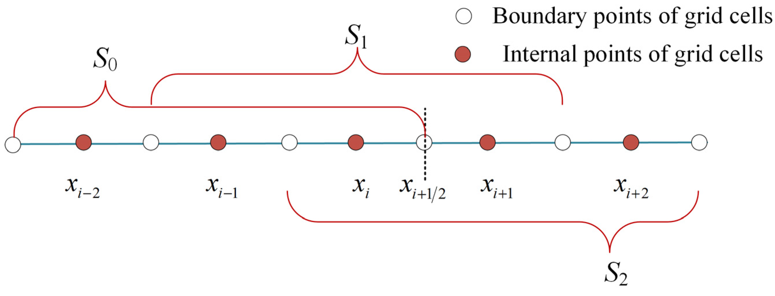
3.2. Fifth-Order WENO Scheme Flux Reconstruction

According to Equation (7), the numerical flux can be obtained by summing the positive and negative parts, while the following template is chosen for the positive flux F + ( U i ) : S 0 = x i 2 , x i 1 , x i , S 1 = x i 1 , x i , x i + 1 , S 2 = x i , x i + 1 , x i + 2 . Figure 2 shows the location of the templates.
From the above template, the flux reconstruction method of the fifth-order WENO scheme can be obtained as
f 0 n = 1 3 F i 2 n 7 6 F i 1 n + 11 6 F i n
f 1 n = 1 6 F i 2 n + 5 6 F i 1 n + 1 3 F i n
f 2 n = 1 3 F i 2 n + 5 6 F i 1 n 1 6 F i n
The above three templates are employed for weighted reconstruction in the actual calculation, and the weights can be determined using the template smoothness function. This paper employs the template smoothness function I S k ± proposed by Vukovic and Sopta [15].
I S k + = α = 1 3 x i 1 / 2 x i + 1 / 2 Δ x 2 α 1 d α f k ( x ) d x α 2 d x   ,   ( k = 0 , 1 , 2 )
Bringing f k n from Equations (8)–(10) into Equation (11) gives
I S 0 + = 13 12 F i 2 n 2 F i 1 n + F i n 2 + 1 4 F i 2 n 4 F i 1 n + 3 F i n 2
I S 1 + = 13 12 F i 1 n 2 F i n + F i + 1 n 2 + 1 4 F i 1 n + 0 F i n F i + 1 n 2
I S 2 + = 13 12 F i n 2 F i + 1 n + F i + 2 n 2 + 1 4 3 F i n 4 F i + 1 n + F i + 2 n 2
where the weighting factor ω k is defined as
ω k = β k i = 1 3 β k
where β k = C k ( ε + I S k + ) 2 , ( k = 0 , 1 , 2 ) , and linear combination coefficients are chosen as
C 0 = 0.3 , C 1 = 0.6 , C 2 = 0.1
Based on the template smoothness function, the positive vector flux expression can be derived as
F i + 1 / 2 + ( U i ) = k = 0 2 ω k I S k + ( F i 2 n , F i 1 n , F i n , F i + 1 n , F i + 2 n )
Similarly, the negative flux expression F i + 1 / 2 ( U i ) can be obtained from the symmetric distribution of the grid interface i + 1 / 2 , while the value of the interface flux F i + 1 / 2 n + 1 ( U i ) at the moment of n + 1 can be obtained from Equation (7).

3.3. Time Layer Discrete Method

The above steps can only find the value of the interface flux at n + 1 times, while the value of the source term s ( u ) is required to calculate the U i n + 1 at n + 1 times. Now, the second-order Runge-Kutta method is employed to solve the initial value problem.
First, the flow term is updated as
U ¯ i n + 1 = U i n + Δ t Δ x ( F ( U i L ) F ( U i R ) )
In the second step, the source item time step is updated as
U i n + 1 = U ¯ i n + 1 + Δ t s ( U ¯ i n + 1 + Δ t 2 s ( U ¯ i n + 1 ) )

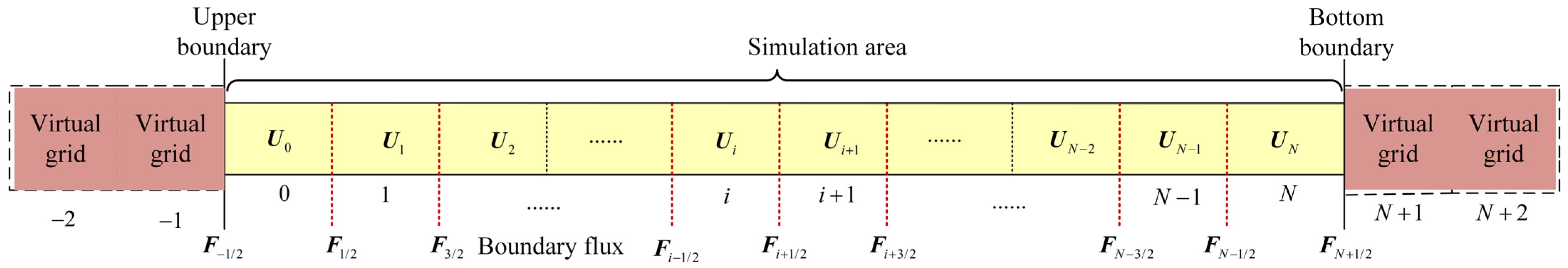
3.4. Boundary Condition Processing

In this paper, the treatment methods of upstream and downstream boundary conditions and pipeline bifurcation boundary are given.

3.4.1. Upstream Boundary Conditions

In actual engineering, the upstream boundary of the pipeline is primarily constant pressure boundary conditions, such as pressure front pool and constant reservoir level. Combining the boundary conditions with MOC gives
v ( 1 , 1 ) n = g c h ( 1 , 1 ) n h ( 1 , 0 ) + v ( 1 , 0 ) ( 1 + g Δ t sin θ c f Δ t 2 D 1 v ( 1 , 0 ) ) h ( 1 , 0 ) = h 0
where h 0 is the upstream constant water pressure and c is the pipeline pressure wave speed.

3.4.2. Downstream Boundary Conditions

The downstream boundary can be the flow rate boundary, flow boundary, or valve boundary. The downstream flow rate is given as v ( i , N ( i ) ) or flow rate as v ( i , N ( i ) ) = Q ( i , N ( i ) ) / A i for the flow rate boundary or flow boundary (Here i represents the pipe number of the pipe network, the same as below). Now, the head at the end of the pipe can be calculated as
h ( i , N ( i ) ) = h ( i , N ( i ) 1 ) n 1 v ( i , N ( i ) ) c i g + v ( i , N ( i ) 1 ) n 1 c i g + Δ t sin θ f Δ x v ( i , N ( i ) 1 ) n 1 2 g D i
Based on the MOC at the boundary and the orifice outflow law, the relationship between head and flow velocity under a valve boundary condition can be determined as
v ( i , N ( i ) ) = v m h 0 τ j h ( i , N ( i ) )
where v m stands for the valve fully open valve at the average flow rate, h 0 stands for the pipeline constant flow state at the valve head, and τ j is the valve opening degree.
To obtain the upstream and downstream boundary flux values F 1 / 2 and F N + 1 / 2 , the virtual boundary values outside the cell inside the pipe should be determined. The dummy grid technique proposed by Mohamed et al. [31] is employed in this paper to improve the computational efficiency while ensuring the accuracy of the results. As shown in Figure 1, for the upstream constant pressure boundary, we have U 2 = U 1 = F 1 / 2 , while for the downstream flow velocity boundary or valve boundary, we have U N + 2 = U N + 1 = F N + 1 / 2 .

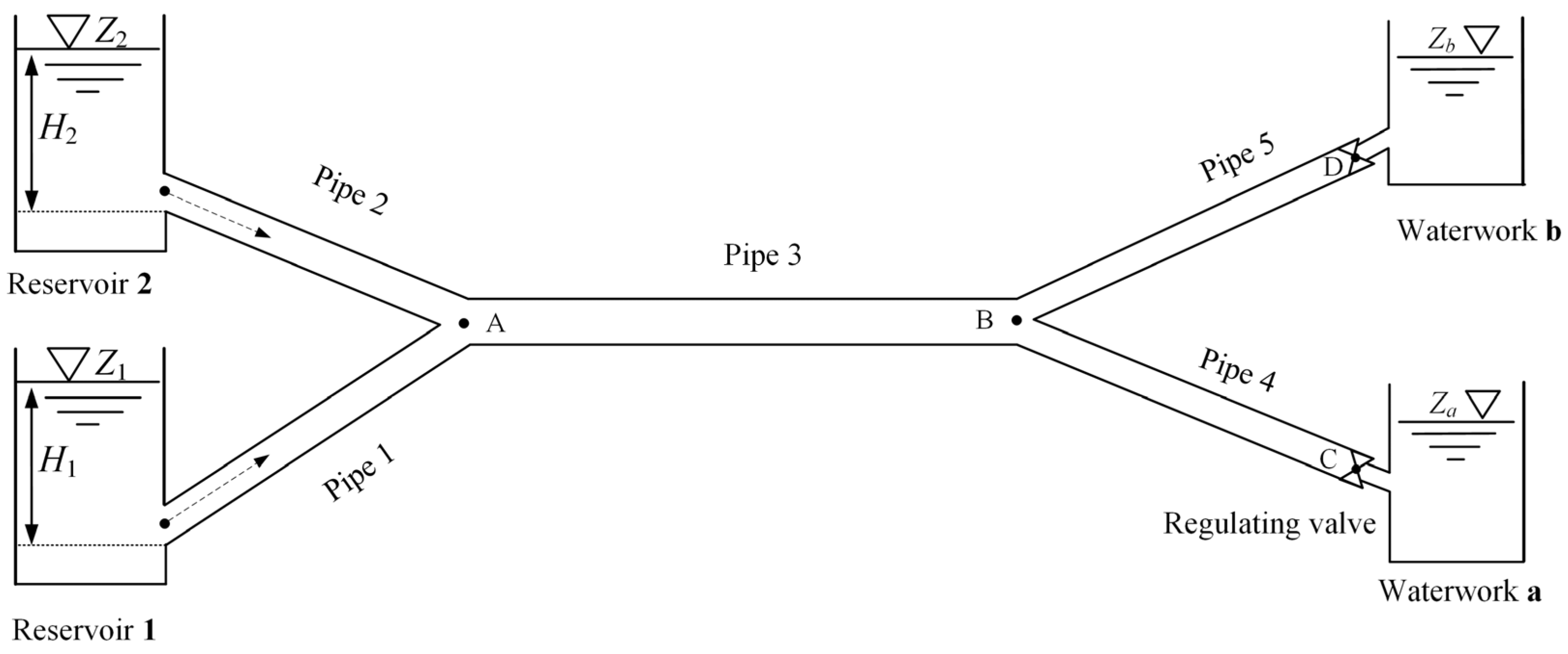
3.4.3. Bifurcated Pipe Interface Handling

When there is a bifurcation in the water delivery system, as shown in Figure 3, it can be handled as the following.
According to the positive characteristic line of pipe A and the negative characteristic line of pipes B and C, we have
h ( A , N ( A ) ) + c A g v ( A , N ( A ) ) = h ( A , N ( A ) 1 ) n 1 + v ( A , N ( A ) 1 ) n 1 c A g + Δ t sin θ A f Δ x v ( A , N ( A ) 1 ) n 1 2 g D A h ( B , 0 ) c B g v ( B , 0 ) = h ( B , 1 ) n 1 v ( B , 1 ) n 1 c B g + Δ t sin θ B f Δ x v ( B , 1 ) n 1 2 g D B h ( C , 0 ) c C g v ( C , 0 ) = h ( C , 1 ) n 1 v ( C , 1 ) n 1 c C g + Δ t sin θ C f Δ x v ( C , 1 ) n 1 2 g D C
The following relation can be obtained from the conservation of flow at the bifurcation and the equal head relationship.
A A v ( A , N ( A ) ) = A B v ( B , 0 ) + A C v ( C , 0 )
h ( A , N ( A ) ) = h ( B , 0 ) = h ( C , 0 )
Equations (23)–(25) should be solved to derive the flow rate and head value at the bifurcation connection of the corresponding moment. If there are more than three sections of pipes connected at the bifurcation, referring to this paper, the number of pipes should be expanded for calculation.

4. GPU Acceleration Implementation Method

Since the pipeline length can be hundreds of kilometers for large water transmission projects, traditional CPU computing architecture is time-consuming and inefficient. With the introduction of GPU acceleration technology, the model calculation efficiency can be significantly improved with minimal loss of model accuracy, ensuring both calculation accuracy and efficiency.

4.1. CPU and GPU Related Parameters

Due to the rapid development of science and technology, the CPU and GPU are changing year by year, while different models of GPU graphics cards have different acceleration effects. The CPU and GPU used in the model are new products in recent years. The CPU is the latest Core series of 10th-generation machines, and the GPU contains 1536 CUDA cores. Table 1 shows the specific key parameters of the CPU and GPU.

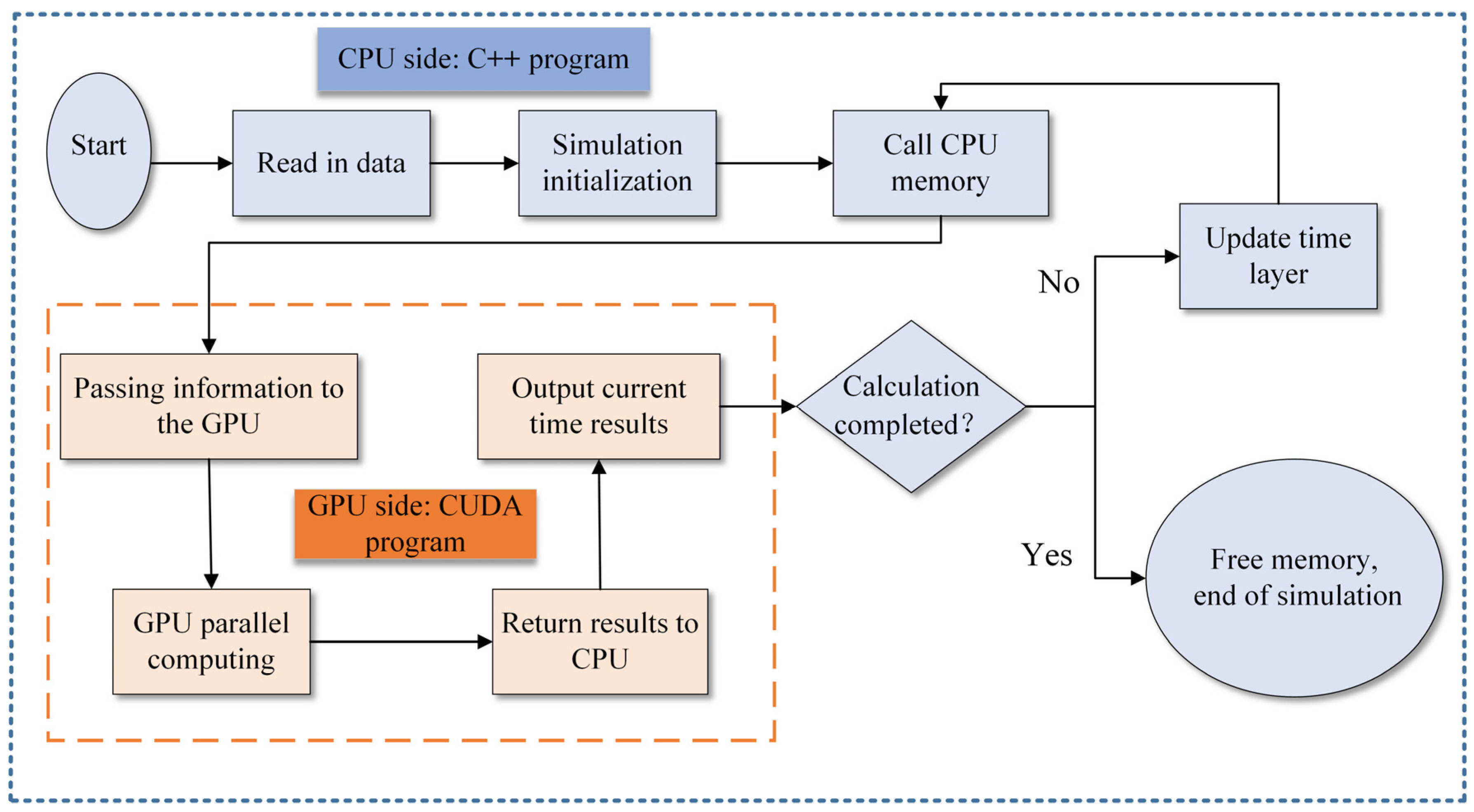
4.2. GPU Accelerated Parallel Computing Process

The model adopts C++ and CUDA language programming to implement the GPU parallel acceleration process. The initial data is stored and initialized on the CPU side, and the cudaMemcpy function is utilized to transfer the computational data to the GPU side as fast as possible, and the GPU threads are called through the kernel function for parallel processing. Figure 4 depicts the specific computation flow.

5. Model Validation and Case Analysis

To evaluate the model’s computational accuracy and efficiency, this paper selects typical working conditions for simulation and validation. It selects the MOC and the first-order and second-order Godunov schemes [10] for comparison and analysis. The Courant number sensitivity of the model is qualitatively verified through the dissipation analysis of different schemes under the same Courant number. By increasing the number of grids, the acceleration effect of the GPU technology in dividing different grids is studied.

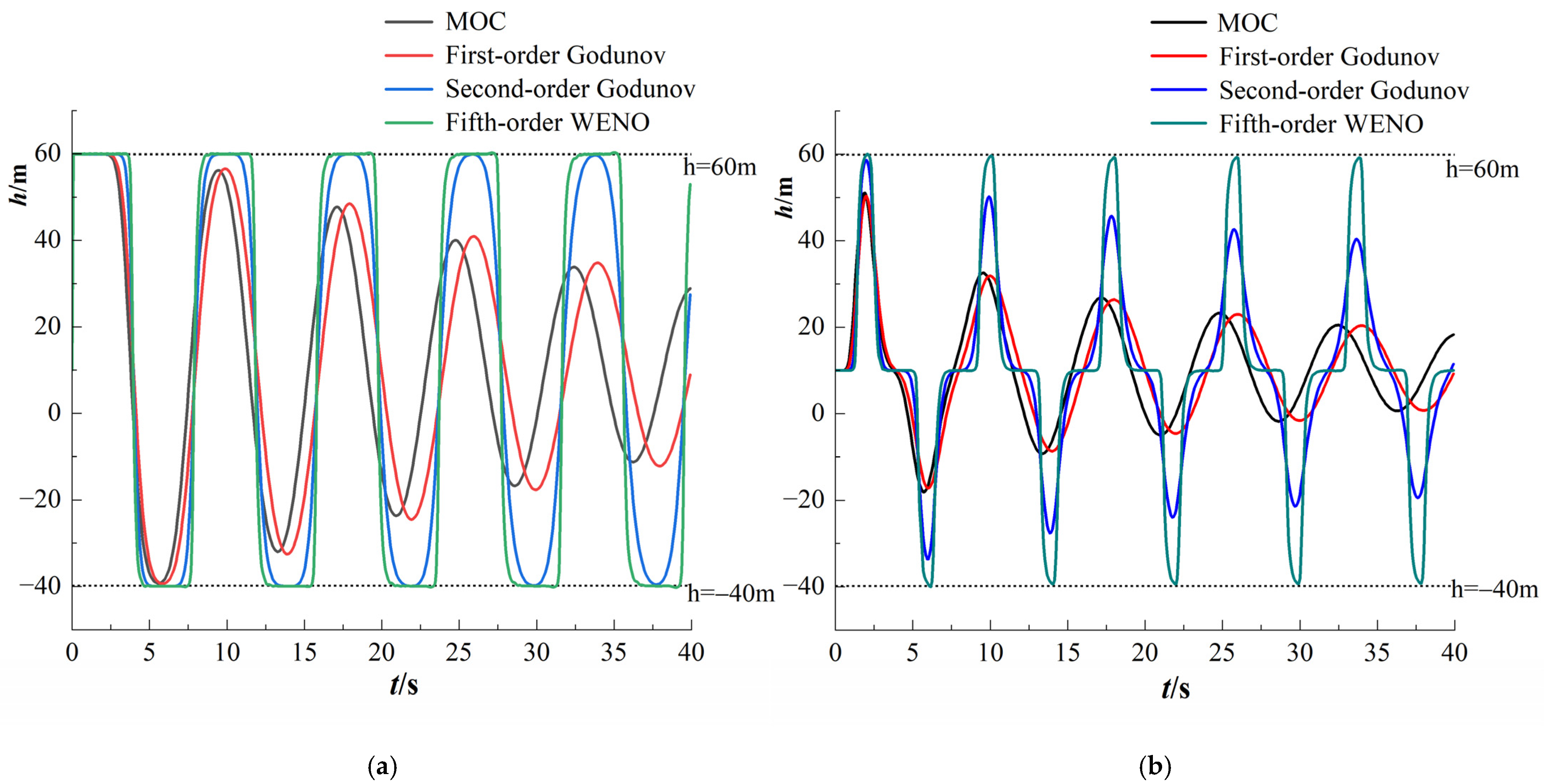
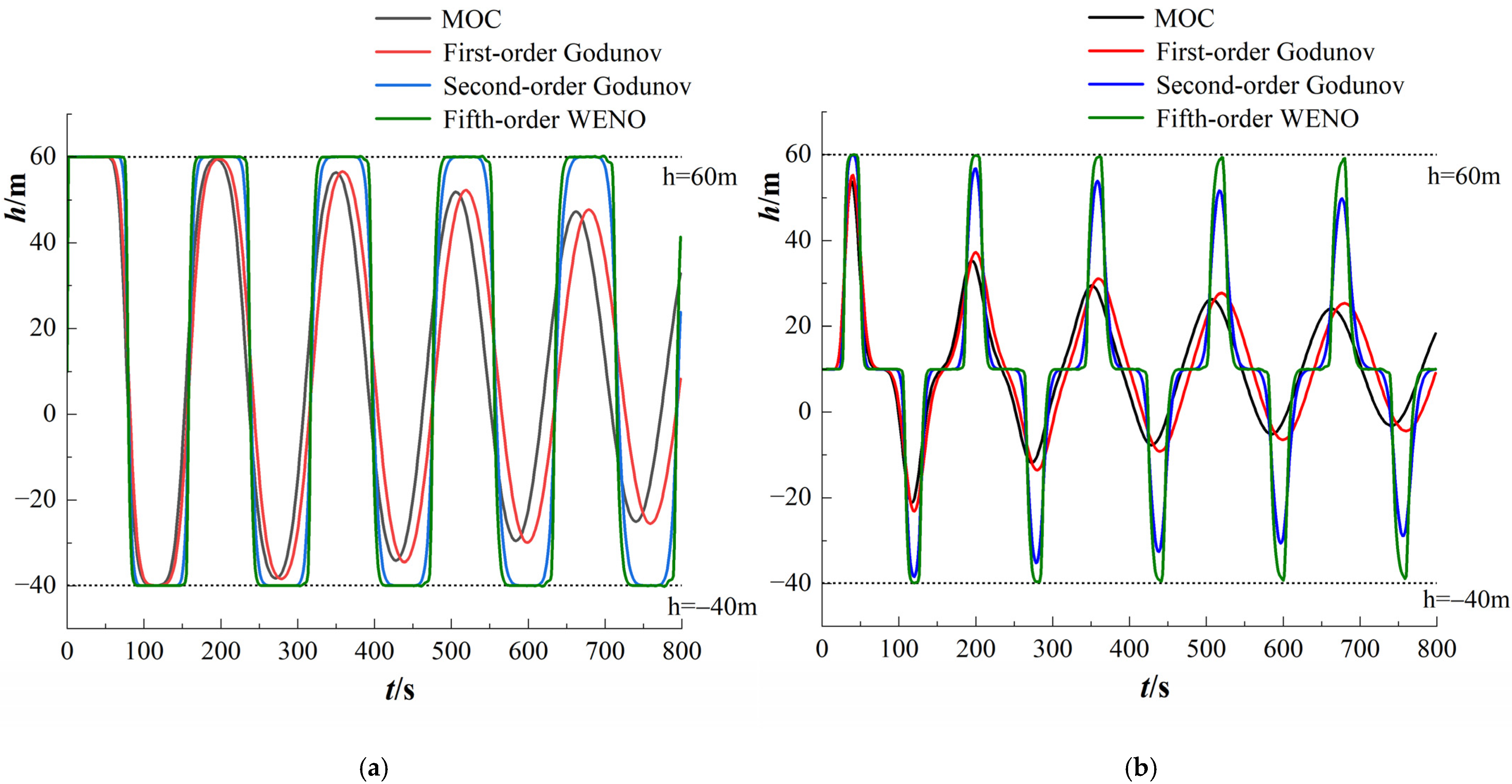
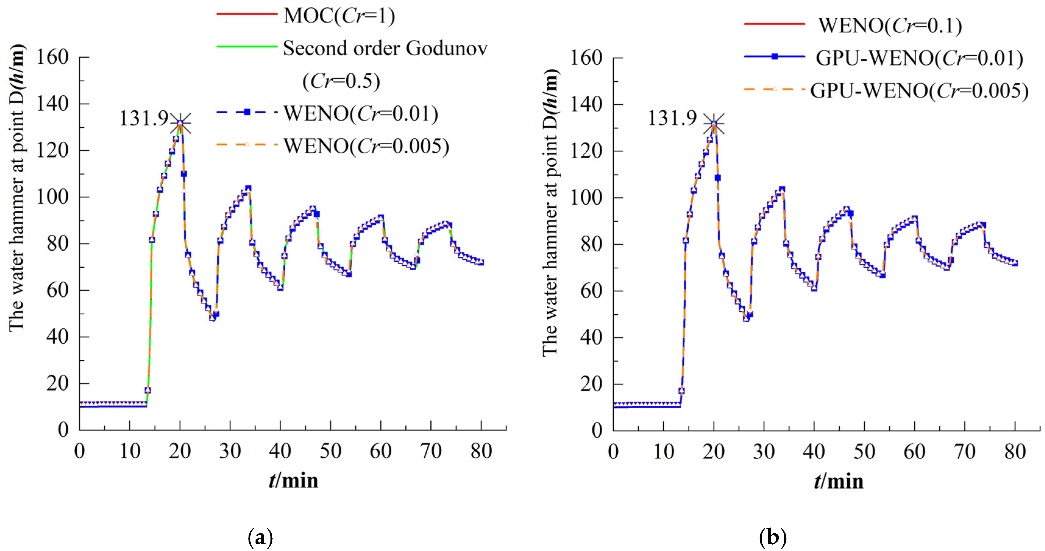
5.1. Parameter Sensitivity Analysis

By calculating and evaluating the numerical dissipation and surge intermittent capture performance of the pressure wave curve at the pipe’s valve at different Courant numbers, the sensitivity of different simulation methods to the Courant number is verified.
Assuming that the two calculation conditions are recorded as Case 1 and Case 2, the pipeline length is 1960 m and 39,200 m, the calculation time is 40 s and 800 s, the grid number is 20 and 40, and the Courant number is 0.1 and 0.01, respectively. Other parameters are the same. The pipe diameter is 1.0 m, the initial flow velocity is 0.5 m/s, the upstream constant water level is 10 m, the wave speed is 980 m/s, and the gravitational acceleration is 9.806 m/s2. The viscous term is ignored, so the roughness of the pipe is 0, and the end valve is suddenly closed.
Figure 5 shows the pressure fluctuation characteristics at the end valve and the 540 m upstream of the pipeline when the model Courant number is 0.1 and the model grid is 20 (case 1). According to the Joukowsky theorem, the change value of water hammer pressure:
Δ h = c Δ v g = 980 × 0.5 9.806 = 49.97   m
The maximum pressure is 59.97 m, the minimum pressure is −39.97 m, and the phase length (the time for traveling one wavelength) of the pressure wave is T = 2 l / c = 2 × 1960 ÷ 980 = 4   s .
As shown in Figure 5, the calculation results of the MOC and the first-order Godunov scheme indicate significant numerical dissipation with increasing time, while the peak pressure waves captured by both schemes are decreasing. The extreme value of the pressure wave at the end valve can be captured accurately during the calculation period using the second-order Godunov scheme. The calculation results at 540 m upstream exhibit a significant error, and the scheme’s numerical dissipation is still more severe. Simultaneously, the second-order Godunov scheme cannot capture the abrupt interruptions. In contrast, the fifth-order WENO scheme accurately captures the actual pressure wave peak and provides performance superior to the other three schemes in capturing the abrupt interruptions of the excitation wave. Figure 5a shows that the second-order Godunov scheme captures a complete excitation interruption with a response time of about 4 s, while the fifth-order WENO scheme captures a complete interruption within 1 s. Besides, the non-physical oscillations generated by the fifth-order WENO scheme are so minimal that their impact on the actual results can be neglected.
Figure 6 shows the pressure fluctuation characteristics when the Courant number is taken as 0.01 and the model grid is 40 (Case 2). Similarly, the pressure change value is Δ h = c Δ v / g = 49.97   m , and the phase length of the pressure wave is T = 2 l / c   = 2 × 39200 ÷ 980 = 80   s . Compared with Figure 5, the numerical dissipation of the MOC and the first-order Godunov scheme decreases slightly by increasing the number of computational grids. However, the scheme cannot capture the pressure wave extremes after 100 s, and the scheme calculation results are almost distorted. The second-order Godunov scheme can better capture the intermittent excitation waves and slightly reduce the dissipation of the scheme values. The fifth-order WENO scheme has no significant nonphysical oscillations and numerical dissipation while maintaining high performance in capturing intermittent excitation waves. In summary, the fifth-order WENO scheme has lower numerical dissipation and better intermittent capture capability than the traditional MOC and Godunov scheme for calculating water hammer waves in pipes with low Courant number conditions.

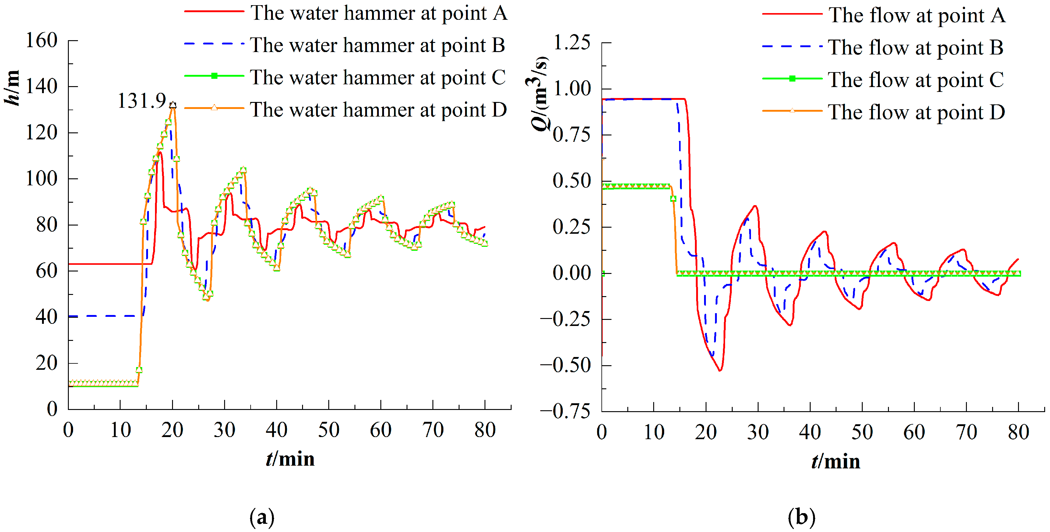
5.2. Model Application and GPU Acceleration Performance Evaluation

The idealized long-distance water pipeline network shown in Figure 7 is constructed to evaluate the simulation’s computational accuracy and the GPU program’s acceleration effect. It is assumed that all the pipelines are long-distance transmission pipes of several tens of kilometers, and points A and B are the branch points of the trig point. The relative elevation of the upstream reservoir constant water level Z1 and Z2 and the downstream water level Za and Zb are 85 m and 5 m, respectively, while the regulating valve at the end of the pipeline is closed by linear variation with a closing time of the 60 s. The MOC and second-order finite volume Godunov scheme are employed to validate the model. The calculation time step is taken as 0.01 s, and the gravitational acceleration is chosen as 9. 806 m/s2. The pipeline model parameters are shown in Table 2.

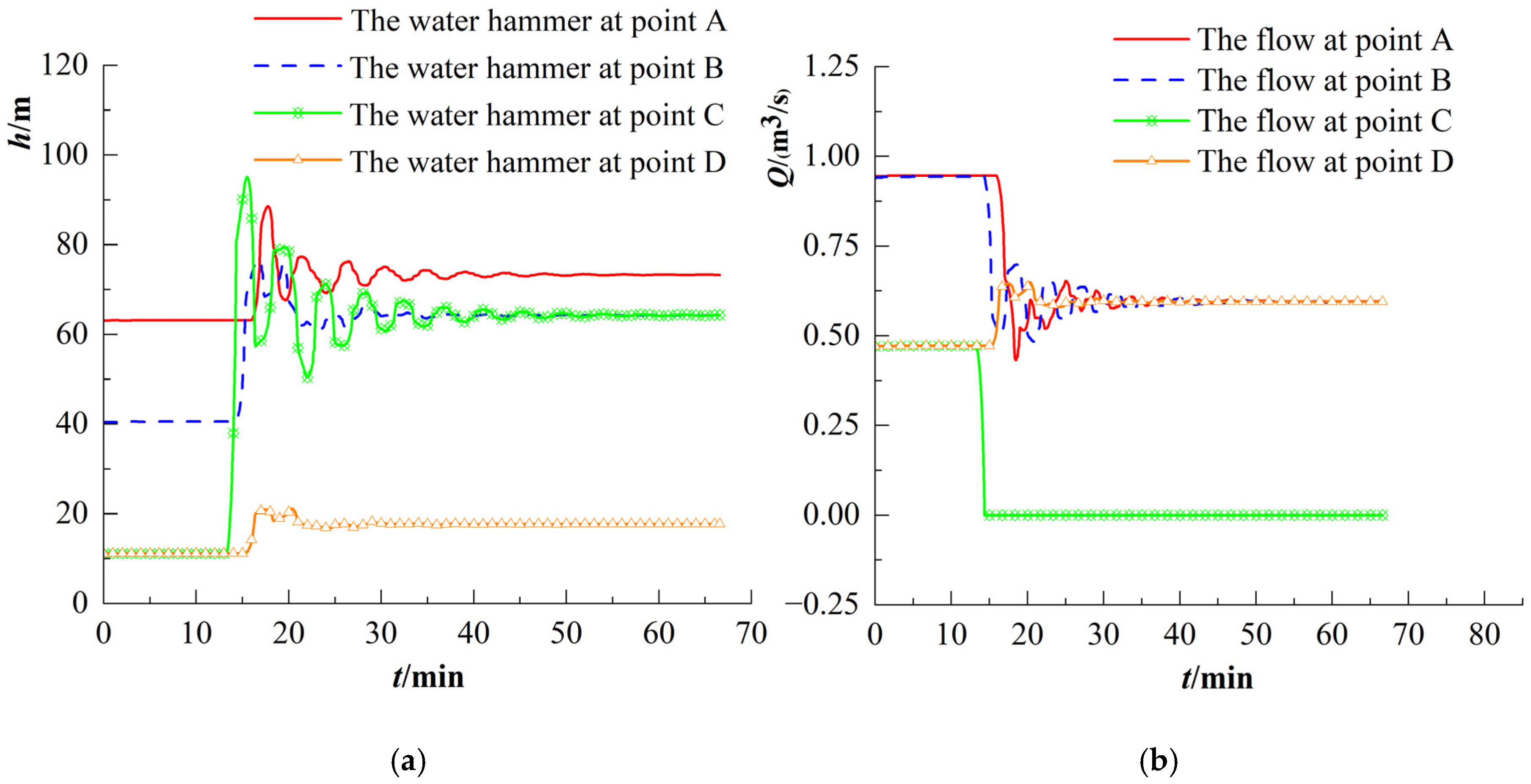
5.2.1. Comparative Analysis of the Results of Different Simulation Methods

Figure 8a shows the process of pressure wave curve change at valve C when the end valves C and D are simultaneously closed for the working condition shown in Figure 7. The working condition first runs steadily for 800 s, and then the valve closes linearly within the 60 s. This paper adopts the fifth-order WENO finite-volume method to take 0.01 and 0.005, respectively. As shown in Figure 8a, the calculation results of different schemes are almost the same, and the error of the extreme value point is within 1‰ when the WENO scheme and the MOC take 0.005. This means that the fifth-order WENO scheme for solving the pipeline water hammer wave can achieve a high accuracy under a very low Courant number. Figure 8b compares the solution results after taking GPU acceleration with the CPU program’s results. The GPU is programmed with double-precision floating-point numbers to ensure calculation accuracy. The maximum error between the calculation result and the CPU program calculation result is 0.5‰, significantly below the allowable error in actual engineering.
Figure 9 shows the flow and water hammer wave variations at different locations when the end valves C and D are simultaneously closed. As shown in Figure 9, due to the symmetry of points C and D location and the simultaneous closure of the valve, the pressure wave curves at valves C and D overlap entirely. Simultaneously, after the valve is closed linearly, the water hammer pressure wave reaches its maximum value (131.9 m). The flow rate at A gradually decreases to 0 with the closure of the valve, while the flow rate at B and C still decrease cyclical in the fluctuation changes due to the role of pipe friction, which gradually decreases the amplitude of fluctuations. Figure 10 shows the flow and pressure head variations at different locations when the valve is closed only at C (linear closure within the 60 s). As shown in Figure 10a, after closing valve C, the pressure head at C suddenly rises, and its peak reaches 95 m, then oscillates down and stabilizes at 64.3 m. After about 40 min, due to the horizontal arrangement of the pipe, the flow rate in pipe 4 drops to zero, while the pressure head at point C is equal to that at point B. The maximum pressure head generated by the whole process system is still at the end of valve C. It can be seen that the downstream valve is still the most likely place to generate damage, even for a complex bifurcated piping system.

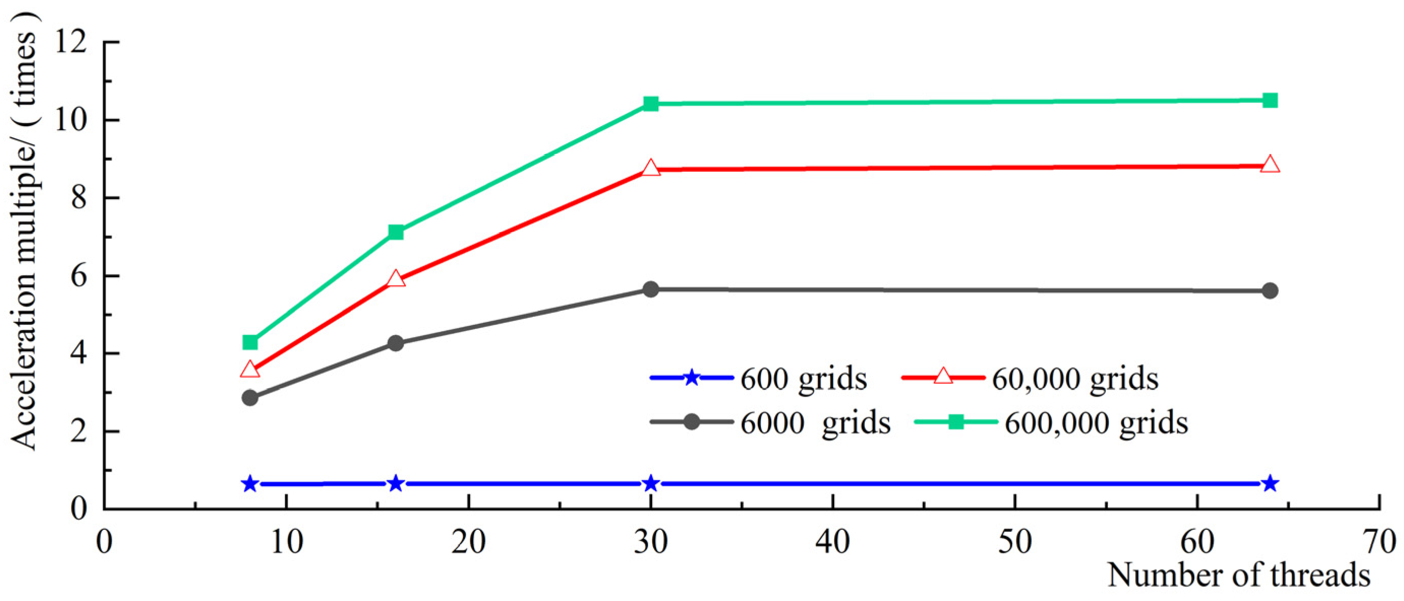
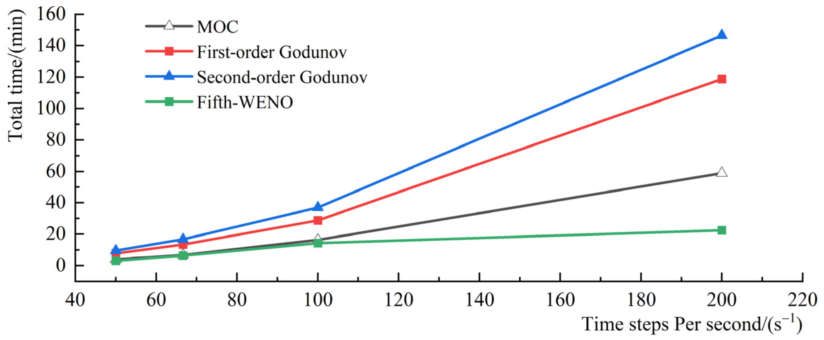
5.2.2. Analysis of Model Computation Efficiency and GPU Acceleration Performance

The water hammer change process at the end valve was calculated in time steps of 0.02 s, 0.015 s, 0.01 s, and 0.005 s. The model’s computational efficiency can be derived by analyzing the computational time consumed by the different schemes, with a computational time of 4800 s. According to the CFL constraint, the MOC and the first-order Godunov scheme should meet Cr = 1, while the second-order Godunov scheme takes Cr = 0.5 to obtain the best calculation effect [10], and the proposed fifth-order WENO finite volume scheme can meet Cr > 0.01. The total computation times for different schemes are presented in Table 3 and Figure 11. According to Table 3, the second-order Godunov scheme takes the highest time, while the MOC and the first-order Godunov scheme take the middle time, and the WENO scheme takes the least time for different time steps, while the Courant number meets the scheme requirements. The fifth-order WENO scheme takes 35% to 90% of the MOC and 15% to 39% of the time of the second-order Godunov scheme when the calculation accuracy is guaranteed and the appropriate Courant number is chosen. It can be concluded that the fifth-order WENO finite volume scheme proposed for the water hammer solution model can significantly improve computational efficiency.
The computational time consumption of CPU programs and GPU programs at different grids was analyzed to evaluate the acceleration effect of the GPU-WENO scheme. The CPU model is Intel(R) Core (TM) i7-10700, and the GPU graphics card is NVIDIA GeForce GTX 1660Ti, and both of them are the latest electronic products in recent years. Still using the ideal operating conditions shown in Figure 7, the pressure wave variation during sudden closure of the end valve was calculated for a total time of 48 s, as presented in Table 4. As shown in Table 4, when the grid number is uniformly divided into 600 and the grid length is 400 m, the single-threaded computation efficiency of the 8-core CPU is higher than that of the GPU. The reason is that the number of CPU program cycles is small, and the CPU core performance can be fully utilized for the small number of grids, while the GPU program is so time-consuming compared to the CPU program because the internal data is copied from the host side to the device side and then copied from the device side to the host side after completing the calculation. The computational efficiency of the GPU program is significantly higher than that of the CPU program when the number of grids reaches thousands and above. At this point, the CPU program’s large number of round-robin calculations is a critical factor in the program’s time consumption, while the efficiency of the GPU is superior to the CPU program by calling multiple threads on the kernel block to perform parallel calculations. Figure 12 shows that when the number of threads reaches 32 or more, the GPU acceleration effect does not change with the increase of threads, indicating that for engineering problems within hundreds of thousands of grids, 32 threads can achieve the best acceleration effect. Besides, the acceleration effects of different graphics cards are significantly different. This model employs the NVIDIA GeForce GTX 1660Ti graphics card, while the acceleration effect can be more than 13 times compared with a single CPU program by using GPU parallel computing technology with a grid number of 500,000 and a grid accuracy of 0.4 m. With the GPU-WENO scheme, which has a high application prospect in solving practical engineering problems, the computation speed can easily reach more than tens of times that of the commonly used MOC or differential scheme.

6. Discussion

This study indicates that the high-precision scheme can well simulate the propagation process of the pressure wave in the one-dimensional pipeline system. Compared to the MOC and the second-order Godunov scheme, the fifth-order WENO scheme yields lower numerical dissipation and no spurious oscillations. GPU acceleration technology is introduced, and the acceleration effect is reached more than ten times. These results can be applied to the regulation and control of long-distance water conveyance systems. This study does not consider the effect of adding gas into the pipeline system. This issue will be further studied in the future.

7. Conclusions

Based on the one-dimensional pipeline non-constant flow equation set, the virtual boundary technique is adopted at the upper and lower ends of the model. The bifurcated pipeline boundary solution method is combined with the Lax-Friedrichs splitting method for flux decomposition, and the time term is discretized by the second-order Runge-Kutta method. Moreover, a fifth-order WENO finite volume scheme water hammer solution model is established for the long-distance water transmission system. The key results are as follows.
(1) The model is verified to ensure low numerical dissipation and lack of spurious oscillations at tiny Courant numbers under ideal conditions. The model is suitable for large and complex water conveyance systems. Compared to the commonly used MOC, the computation load of the model is 35% to 90% less than the MOC and 15% to 39% less than the second-order Godunov scheme while maintaining the accuracy of the results.
(2) Using GPU acceleration technology to accelerate the model, the model can achieve a significant acceleration effect while ensuring accuracy when the number of grids is greater than thousands. As the number of meshes increases, the GPU acceleration effect becomes more and more significant. The study found that GPU with 32 threads can deal with engineering problems within hundreds of thousands of grids with the best acceleration effect.

Author Contributions

Conceptualization, T.M. and G.L.; methodology, T.M. and G.L.; software, T.M.; validation, T.M.; formal analysis, G.L.; resources, T.M.; data curation, T.M.; writing—original draft preparation, T.M.; writing—review and editing, G.L.; supervision, G.L.; project administration, G.L.; funding acquisition, G.L. All authors have read and agreed to the published version of the manuscript.

Funding

This study was funded by the National Natural Science Foundation of China (No. 52079107).

Institutional Review Board Statement

Not applicable.

Informed Consent Statement

Not applicable.

Data Availability Statement

The data that support the findings of this study are available from the corresponding author upon reasonable request.

Conflicts of Interest

The authors declare that they have no conflict of interest. The funders had no role in the design of the study, in the collection, analyses, or interpretation of data, in the writing of the manuscript, or in the decision to publish the results.

Abbreviations

The following symbols are used in this paper:
A Pipe cross-sectional area (m2);
A , A ¯ Coefficient matrix and the linearized coefficient matrix;
c Water hammer wave speed in the pipeline (m);
C 0 , C 1 , C 2 Weighting coefficients;
D Pipe diameter (m);
f Pipeline resistance coefficient;
f 0 n , f 1 n , f 2 n Weighted   reconstruction   template   at   i + 1 / 2   interface   at   time   n ;
F i n , F + , F The   flux   term   at   time   n   at   interface   i , and the positive and negative split flux terms;
g Acceleration due to gravity (m/s2);
h 0 , h 0 Pressure head in the upstream reservoir area and pressure head at the valve at constant flow (m);
h , h ( i , k ) j Water   hammer   pressure   at   node   k   at   segment   i   at   time   j (m);
n Time step;
Q ( i , N ( i ) ) Flow   value   at   node   N   of   section   i in the pipeline;
S 0 , S 1 , S 2 Templates for WENO scheme;
s Source terms;
t Computing time (s);
u Flow variable;
U i , U i L , U i R Mean   value   of   u ,   that   to   left   and   right   of   interface   i + 1 / 2 , respectively;
U i n , U ¯ i n + 1 , U i n + 1 Intermediate flow variables for Runge-Kutta scheme;
v , v ( i , k ) j Velocity   value   at   node   k   at   segment   i   at   time   j (m/s);
v ¯ , v m Average velocity and maximum velocity (m/s);
x Distance from the most upstream (m);
Δ x Incremental   element   in   x   ;
α Maximum eigenvalue of Jacobian matrix;
β 0 , β 1 , β 2 Linear combination coefficients;
τ j Valve   opening   at   time   j ;
λ ± Positive and negative eigenvalues of the Jacobian matrix;
θ The angle between the pipe and horizontal plane;
ω 0 , ω 1 , ω 2 Linear combination coefficient weight;
I S 0 + , I S 1 + , I S 2 + Template smoothness functions;
The following abbreviations are used in the text:
MOCMethod of characteristics;
WENOWeighted Essentially non-oscillatory;
GPUGraphic Processing Unit;
CPUCentral Processing Unit;
TVDTotal Variation Diminishing;
ENOEssentially non-oscillatory;
CUDACompute Unified Device Architecture;

References

  1. Wu, D.; Yang, S.; Wu, P.; Wang, L. MOC-CFD Coupled Approach for the Analysis of the Fluid Dynamic Interaction between Water Hammer and Pump. J. Hydraul. Eng. 2015, 141, 06015003. [Google Scholar] [CrossRef]
  2. Adamkowski, A.; Henclik, S.; Janicki, W.; Lewandowski, M. The influence of pipeline supports stiffness onto the water hammer run. Eur. J. Mech. B/Fluids 2017, 61, 297–303. [Google Scholar] [CrossRef] [Green Version]
  3. Boran, Z.; Wuyi, W.; Mengshan, S.J.W. Experimental and Numerical Simulation of Water Hammer in Gravitational Pipe Flow with Continuous Air Entrainment. Water 2018, 10, 928. [Google Scholar]
  4. Harten, A. High Resolution Schemes for Hyperbolic Conservation Laws. J. Comput. Phys. 1983, 49, 357–393. [Google Scholar] [CrossRef] [Green Version]
  5. Wylie, E.B.; Streeter, V.L. Fluid Transients in Systems; Prentice Hall: Hoboken, NJ, USA, 1993. [Google Scholar]
  6. Chaudhry, M.H.; Hussaini, M.Y. Second-Order Accurate Explicit Finite-Difference Schemes for Waterhammer Analysis. J. Fluids Eng. Trans. Asme 1985, 107, 523–529. [Google Scholar] [CrossRef]
  7. Wan, W.; Huang, W. Water hammer simulation of a series pipe system using the MacCormack time marching scheme. Acta Mech. 2018, 229, 3143–3160. [Google Scholar] [CrossRef]
  8. Wylie, E.B.; Stoner, M.A.; Streeter, V.L. Network System Transient Calculations by Implicit Method. Soc. Pet. Eng. J. 1971, 11, 356–362. [Google Scholar] [CrossRef]
  9. Zhao, L.; Yang, Y.; Wang, T.; Han, W.; Wu, R.; Wang, P.; Wang, Q.; Zhou, L.J.W. An Experimental Study on the Water Hammer with Cavity Collapse under Multiple Interruptions. Water 2020, 12, 2566. [Google Scholar] [CrossRef]
  10. Zhao, M.; Mohamed, S.; Ghidaoui, M.A. Godunov-Type Solutions for Water Hammer Flows. J. Hydraul. Eng. 2004, 130, 341–348. [Google Scholar] [CrossRef]
  11. Waagan, K. A positive MUSCL-Hancock scheme for ideal magnetohydrodynamics. J. Comput. Phys. 2009, 228, 8609–8626. [Google Scholar] [CrossRef] [Green Version]
  12. Harten, A.; Engquis, B.; Osher, S.; Chakravarthy, S.R. Uniformly high order accurate essentially non-oscillatory schemes, III. J. Comput. Phys. 1987, 71, 231–303. [Google Scholar] [CrossRef]
  13. Li, X.; Li, G.; Ge, Y. Improvement of third-order finite difference WENO scheme at critical points. Int. J. Comput. Fluid Dyn. 2019, 34, 1–13. [Google Scholar] [CrossRef]
  14. Jiang, G.; Shu, C. Efficient Implementation of Weighted ENO Schemes. J. Comput. Phys. 1996, 126, 202–228. [Google Scholar] [CrossRef] [Green Version]
  15. Vukovic, S.; Sopta, L. ENO and WENO Schemes with the Exact Conservation Property for One-Dimensional Shallow Water Equations. J. Comput. Phys. 2002, 179, 593–621. [Google Scholar] [CrossRef]
  16. Liu, X.; Osher, S.; Chan, T.F. Weighted essentially non-oscillatory schemes. J. Comput. Phys. 1994, 115, 200–212. [Google Scholar] [CrossRef] [Green Version]
  17. Zhu, J.; Qiu, J. A new fifth order finite difference WENO scheme for solving hyperbolic conservation laws. J. Comput. Phys. 2016, 318, 110–121. [Google Scholar] [CrossRef]
  18. Li, X.; Li, G.; Ge, Y. High-accuracy numerical simulations on dam break flows with improved weno scheme. Chin. J. Hydrodyn. 2019, 34, 512–519. [Google Scholar]
  19. Li, G.; Li, X.; Li, P.; Cai, D. An improved third-order finite difference weighted essentially nonoscillatory scheme for hyperbolic conservation laws. Int. J. Numer. Methods Fluids 2020, 92, 1753–1777. [Google Scholar] [CrossRef]
  20. Choi, H.; Lee, J. Efficient Use of GPU Memory for Large-Scale Deep Learning Model Training. Appl. Sci. 2021, 11, 10377. [Google Scholar] [CrossRef]
  21. Zhang, J.; Chen, H.; Cao, C. A graphics processing unit-accelerated meshless method for two-dimensional compressible flows. Eng. Appl. Comput. Fluid Mech. 2017, 11, 526–543. [Google Scholar] [CrossRef] [Green Version]
  22. Tutkun, B.; Edis, F.O. An implementation of the direct-forcing immersed boundary method using GPU power. Eng. Appl. Comput. Fluid Mech. 2016, 11, 15–29. [Google Scholar] [CrossRef] [Green Version]
  23. Wang, Y.; Zhao, Y.; Jiang, J.; Zhang, H.J.A.S. A Novel GPU-Based Acceleration Algorithm for a Longwave Radiative Transfer Model. Appl. Sci. 2020, 10, 649. [Google Scholar] [CrossRef] [Green Version]
  24. Liang, Q.; Xia, X.; Hou, J. Catchment-scale High-resolution Flash Flood Simulation Using the GPU-based Technology. Procedia Eng. 2016, 154, 975–981. [Google Scholar] [CrossRef] [Green Version]
  25. Meng, W.; Cheng, Y.; Wu, J.; Yang, Z.; Shang, S.; Yang, F. GPU parallel acceleration of transient simulations of open channel and pipe combined flows. IOP Conf. Ser. Earth Environ. Sci. 2019, 240, 052025. [Google Scholar] [CrossRef]
  26. Darian, H.M.; Esfahanian, V. Assessment of WENO schemes for multi-dimensional Euler equations using GPU. Int. J. Numer. Methods Fluids 2014, 76, 961–981. [Google Scholar] [CrossRef]
  27. Parna, P.; Meyer, K.; Falconer, R. GPU driven finite difference WENO scheme for real time solution of the shallow water equations. Comput. Fluids 2018, 161, 107–120. [Google Scholar] [CrossRef] [Green Version]
  28. Toro, E.F. Riemann Solvers and Numerical Methods for Fluid Dynamics; Springer: Berlin/Heidelberg, Germany, 1997. [Google Scholar]
  29. Toro, E.F. Shock-Capturing Methods for Free-Surface Shallow Flows; Wiley-Blackwell: Hoboken, NJ, USA, 2001. [Google Scholar]
  30. Castro, M.; Costa, B.; Don, W.S. High order weighted essentially non-oscillatory WENO-Z schemes for hyperbolic conservation laws. J. Comput. Phys. 2011, 230, 1766–1792. [Google Scholar] [CrossRef]
  31. Zerroukat, M.; Chris, R.C. A Finite-Difference Algorithm for Multiple Moving Boundary Problems Using Real and Virtual Grid Networks. J. Comput. Phys. 1994, 112, 298–307. [Google Scholar] [CrossRef]
Figure 1. Schematic diagram of pipeline meshing.
Applsci 12 07350 g001
Figure 2. Computational stencils of WENO.
Applsci 12 07350 g002
Figure 3. Bifurcated pipe interface mesh division diagram.
Applsci 12 07350 g003
Figure 4. GPU acceleration flowchart.
Applsci 12 07350 g004
Figure 5. Comparison of results of different schemes for Cr = 0.1. (a) Comparison of pressure wave curve at value. (b) Comparison of pressure wave curves at 540 m.
Applsci 12 07350 g005
Figure 6. Comparison of results of different schemes for Cr = 0.01. (a) Comparison of pressure wave curve at value. (b) Comparison of pressure wave curves at 10 km.
Applsci 12 07350 g006
Figure 7. Schematic diagram of the long-distance water pipeline.
Applsci 12 07350 g007
Figure 8. Results of different simulation methods. (a) Comparison of accuracy of different methods. (b) Precision comparison of GPU acceleration methods.
Applsci 12 07350 g008
Figure 9. The flow and water hammer wave variations at different locations when the end valves C and D are closed. (a) The water hammer changes with time at different positions. (b) Flow at different locations varies with time.
Applsci 12 07350 g009
Figure 10. The flow and pressure head variations at different locations when the valve is closed only at C. (a) The water hammer changes with time at different positions. (b) Flow at different locations varies with time.
Applsci 12 07350 g010
Figure 11. Comparison of calculation speed of different simulation methods.
Applsci 12 07350 g011
Figure 12. Accelerated rendering with different threads and grid numbers in GPU.
Applsci 12 07350 g012
Table 1. Key parameters of GPU and CPU.
GPU TypeComputational FrameworkNumber of TransistorsNumber of Stream ProcessorsMemory CapacitySingle-Precision Floating-PointVideo Memory Bandwidth
NVIDIA GeForce GTX 1660TiPascal6 billion 600 million15366000 MB4.85 TERAFLOPS288(Gb/s)
CPU TypeComputational FrameworkBasic FrequencyNumber of ThreadsL3 CacheMaximum Memory Support
Intel(R) Core (TM) i7-10700 Comet Lake-S2.90 GHz8 threads16 MB8 GB
Table 2. The pipeline model parameters.
Pipe NumberPipe Length/kmPipe Diameter/mRoughnessWave Speed/(m/s)Initial Flow/(m3/s)
Pipe 139.750.9810.0139960.47
Pipe 239.750.9810.0139960.47
Pipe 399.401.3890.01210000.94
Pipe 459.640.9810.0149940.47
Pipe 559.640.9810.0149940.47
Table 3. The calculation time of different simulation methods.
Time Step (t/s)MOC (t/min)First-Order Godunov (t/min)Second-Order Godunov (t/min)Fifth-Order WENO (t/min)
0.0203.997.769.553.05
0.0156.7213.4716.756.34
0.01016.3128.7336.9014.36
0.00559.00118.75146.5422.47
Table 4. Effect analysis table of GPU acceleration.
Number of GridsGrid Accuracy/(m)CPU-WENO (t/s)GPU-WENO (t/s)Acceleration Ratio/(Times)
Number of ThreadsNumber of Threads
81632648163264
6004004.445.225.215.195.220.850.850.860.85
60004048.1611.556.335.205.234.177.619.269.21
6 × 1044479.2491.2857.8847.2746.965.258.2810.1410.21
6 × 1050.44731.08793.81502.24358.96354.395.969.4213.1813.35
Publisher’s Note: MDPI stays neutral with regard to jurisdictional claims in published maps and institutional affiliations.

