Improved Calculation Method for Siphon Drainage with Extended Horizontal Sections

Abstract

Slope siphon drainage is a convenient and efficient above-ground drainage method that is free of manual power and can effectively maintain the stability of potential landslides and prevent the loss of life and property. The complex engineering topography inevitably requires the use of siphon drains with a total length of more than 150 m and a horizontal section length of more than 80 m, which significantly increases the difficulty of calculating the drainage capacity and thus affects the actual utilization of the project. The traditional siphon flow rate equation does not apply to long-pipe siphon conditions, especially when the lift is close to the limit, and there are significant errors in the calculation results, for which we propose a new calculation method. The proposed method considers both air release and flow-pattern classification. Thirty-six sets of experiments were conducted to validate our proposed calculation method. The results showed that our method not only calculated the siphon flow velocity well but also predicted the main flow pattern in the siphon in the experiment well. Furthermore, the equation for calculating the siphon flow velocity was extended to the siphon operation mode with long horizontal sections.

1. Introduction

Landslide disasters frequently occur in hilly mountainous areas of China, seriously endangering the safety of life and property of residents and road traffic. In addition, the stability of many landslides is closely related to the action of groundwater and is vulnerable to solid rainfall. Therefore, adopting methods such as slope drainage to reduce and control the groundwater level is a necessary technical means to manage landslides.

Under atmospheric pressure, the imbalance of forces caused by the difference in the height of the inlet and outlet causes the physical phenomenon of liquid moving from a lower to a higher and then to a lower level, which is called “siphoning”. Based on this principle, slope siphon drainage technology cleverly uses the ubiquitous atmospheric pressure and the topographic conditions of the slope, which leads to the deeply buried groundwater discharging from the slope, as shown in Figure 1.

Siphon drainage technology is used worldwide, with pipe diameters ranging from millimeters to meters. As early as 1988, Gress designed an automatic siphon drainage system for slopes in a patent [1], and based on this improved patent, he proposed a better choice of 6–10 mm diameter pipes [2]. The team of Bai and Liu explored the use of 10 cm diameter siphons for siphoning agricultural water-saving irrigation and reservoir slope drainage management, while the team of Shang and Sun [3,4,5,6] concentrated on the application of millimeter siphon pipe diameters for potential landslide water table precipitation. In the early stage of siphoning technology applied to slope drainage, air bubble accumulation and consolidation occurred at the top of the tube due to the long-term stoppage of siphoning caused by the dry water period and under the action of several factors. The accumulation of air led to the destruction of the vacuum characteristics at the top of the pipe, which eventually reduced the siphon restarting capacity or even made the siphon device ineffective and reduced the safety of the landslide management project. In a study by Cai et al. [5], reducing the pipe diameter to form a segmental slug flow in the pipe allowed the air bubbles to be discharged from the pipe in time to prevent air accumulation during the siphoning action. The application of siphon technology has significant advantages, such as not requiring power and low construction cost. However, topographic constraints lead to the need for most projects to use siphons longer than 100 m. The increased length of the horizontal section poses a more significant challenge for siphon flow calculation and subsequent engineering application scheduling.

The flow pattern plays a crucial role in the gas–liquid two-phase flow; its flow characteristics affect the pressure drop and energy loss. The models explored in this paper are all air–water two-phase flows in a circular tube. Due to the self-driven nature of siphon flow, the velocity of the gas phase within the fluid does not appear much larger than the velocity of the liquid phase, so the distribution of siphon flow type is relatively single. The Lockhart gas–liquid two-phase flow pattern diagram shows that the siphon flow occurs in millimeter diameter siphons at high-lift conditions. The segmental slug flow and the elastomeric flow are the most significant and long-term applicable flow patterns for the whole pipe section. Segmental slug flow is a complex flow pattern with non-homogeneous, periodic, and random unit length characteristics. At the same time, different types of slug flow in a circular tube will show different characteristics, and the different forms of gas present in the liquid will directly affect the energy and momentum exchange rate. Therefore, it is essential to distinguish the different flow types, especially the segmental slug flow, and to choose an appropriate gas–liquid two-phase motion model to accurately describe the siphoning process and predict the siphoning flow rate.

The hydrodynamics of gas–liquid two-phase flow slug flow patterns in microchannels have received extensive attention in the last few decades and have been studied extensively in the work of Gupta et al. [7,8], Talimi et al. [9], Bandara et al. [10], and Haase et al. [11]. Ratulowski and Chang [12] calculated the pressure drop and film thickness of isolated bubbles and the pressure drop and film thickness of bubble strings in circular and square capillaries in a range of bubble volumes. The hydrodynamic properties involved in slug bubble flow were analyzed in several numerical and experimental studies, including macroscale systems [13,14,15,16,17] and millimeter and micron scales [18,19]. Rocha et al. [20] studied the shape, velocity, and liquid film flow around Taylor bubbles under certain operating conditions and obtained the flow behavior of the slug flow in three typical microchannels. Ratulowski [12] and Suresh et al. [21] performed numerical simulations based on axisymmetric and two-dimensional planar assumptions, and Khan et al. [22] explored the heat transfer and pressure distribution of magnetohydrodynamic thin film by using the Homotopy Analysis Method. In addition, many researchers, such as Giavedoni [23], Heil [24], and Kreutzer [25] investigated the effect of the Reynolds number on the liquid film thickness, shape, and pressure drop of Taylor bubbles. The complete results showed that the bubble liquid film thickness did not vary much with Reynolds number when the Reynolds number was less than 900; however, the liquid film thickness reached the minimum value at a moderate Reynolds number. Among them, the bubbles with high capillary numbers showed the characteristic of a thin head and concave tail, and the bubbles occupied almost the entire cross-section of the tube with a fragile liquid film flowing around them, and the liquid film could be regarded as almost stationary. However, at low capillary numbers, the bubbles had a rounded tail and head, the cross-section occupied the entire cross-section of the tube, and the average velocity of the liquid enclosed in these regions was equal to the bubble velocity, i.e., the gas and liquid flowed like a piston.

2. Preliminary Analysis of the Flow Pattern in the Siphon

According to Henry’s law, the solubility of air is positively related to the ambient air pressure. Under high-lift siphon conditions, the flow velocity in the descending section was greater than the flow velocity in the back of the ascending section, resulting in a significant drop in air pressure in the tube, which gradually exceeded the critical range for air precipitation. The bubbles’ height in the rising section was influenced by several factors, including the total length of the siphon, the diameter of the pipe, and the siphon lift. All other things being equal, the height of the bubbles in the rise section decreased as the siphon lift increased. Similarly, the gravity flow length at the top of the descending section of the siphon during siphon flow was not constant but was influenced by the pipe diameter, pipe length, lift, and descending section length, among other factors. All other things being equal, the gravity flow length of the descending section increased with increasing pipe diameter and increased with increasing lift. Furthermore, due to the difference in flow velocity between the ascending and descending sections, very obvious bubbles were observed in the horizontal section of the high-lift long-pipe siphon, where the 3–5 mm pipe diameter was characterized mainly by segmental slug flow, while the 6.5–8 mm pipe diameter was mainly characterized by elastic or annular flow with occasional bubble flow.

Cai showed that the maximum diameter of the bubble that can maintain a stable structure is about 4.6 mm under stagnant water without boundary conditions. In contrast, in flowing water, the size of the bubble is determined by its force; that is, when its surface tension and the shear stress and mass forces acting on its surface are balanced, the bubble will not break, and its size is unstable. Therefore, the equation proposed by Hinze [26] can be used to estimate the critical size of bubbles in water flow.

$$d_{95}=0.725{\left(\frac{\sigma }{{\rho }_l}\right)}^{\frac{3}{5}}{\left(\frac{1}{\epsilon }\right)}^{\frac{2}{5}}$$

(1)

where $d_{95}$ is the sum of the volume of bubbles more minor than the critical diameter occupies 95% of the total volume of bubbles, ${\rho }_l$ is the density of the liquid, $\sigma$ is the surface tension of the bubble interface, and ε is the energy consumption per unit mass.

In this study, a circular pipe was used for siphon drainage, so the energy consumption in a pipe of length L can be considered as

$$P_u=Q\gamma h_l$$

(2)

where Q is the flow rate, $h_l$ is the head loss of the section, $\gamma$ is the heaviness of the fluid. Then the mass of water in the pipe section is

$$M={\rho }_{l}AL=\frac{{\rho }_{l}QL}{v_l}$$

(3)

where A is the cross-sectional area of the pipe and $v_l$ is the average flow velocity of the test section. Dividing Equation (2) by Equation (3), the energy consumption per unit mass for pipe flow can be expressed as

$$\epsilon =\frac{g{h}_l{v}_l}{L}$$

(4)

According to the Darcy formula,

$$h_l=\lambda \frac{L}{d}\frac{v_l^2}{2g}$$

(5)

where D is the siphon diameter, $v_l$ is the average flow velocity of the test section, and λ is the along-travel resistance coefficient (determined by the Reynolds number Re). Substituting Equation (5) into Equation (4) yields

$$\epsilon =\frac{\lambda v_l^3}{2D}$$

(6)

Therefore,

$$d_{95}=0.1497449\times {\left(\frac{D}{v_l}\right)}^{\frac{4}{5}}$$

(7)

Hinze’s theory states that the presence of bubbles in a siphon pipe is directly related to the pipe diameter and the average fluid flow velocity in the pipe, which is further influenced by the lift, pipe length, and other factors. It can be seen that in a 200 m-long distance siphon drain with a pipe diameter of 5 mm when the lift is less than 3.3 m, more than 95% of the bubbles in the flow state can reach a stable diameter of 5 mm or more, as shown in Figure 2. In other words, the air accumulation problem caused by “non-segmental slug flow” can be effectively avoided in a 5 mm-long siphon, and this is confirmed by the flow pattern observed in the test.

For liquid-transport processes, single-phase flow of a whole tube of liquid is the most desirable and most efficient but impossible form of flow in a siphon drainage system. This is determined by the unique physical characteristics of the siphon drainage system: the presence of reverse gravitational motion of the liquid. As liquid gradually rises in the vertical section, the air pressure inside decreases, which, according to Henry’s law, leads to a decrease in the solubility of the gas solute in the liquid, which in turn leads to air precipitation and the formation of bubbles in the tube. Therefore, gas–liquid two-phase flow is inevitable in the siphon drainage process, which also greatly enhances the complexity of siphon drainage theory calculations. In addition, the most direct effect caused by bubbles in the tube is the formation of a non-homogeneous fluid, which leads to momentum transfer with jump characteristics. However, the segmental slug flow formed under different conditions will have different pressure transfer paths and pressure drop magnitudes.

Different types of flow patterns in a circular tube will exhibit different characteristics, and the different forms of gas present in the fluid will directly affect the energy and momentum exchange rates. Therefore, it is essential to distinguish between different flow types and choose an appropriate gas–liquid two-phase motion model to describe and predict the siphoning process accurately. This study focused on improving the computational accuracy of long-pipe siphons, which have more complex and stochastic fluid motion than short-pipe siphons and different flow-rate losses. While the critical analysis surface of the short siphon can be intuitively chosen as the highest point of the siphon based on the energy loss characteristics, the long horizontal siphon will be in a state of continuous energy loss at its highest horizontal position. Therefore, in the process of calculating the siphon flow velocity in the long horizontal section, although the process of air pressure change in the rising section is similar to that in the short tube, the interaction between the fluid and the tube wall in the horizontal section has a considerable effect on the change of flow velocity.

Aditya [27] developed a slug bubble theory model based on lubrication theory and capillary effect theory that can be used to predict the shape and pressure drop of long bubbles in a circular tube in pressure-driven flow. The pressure drop before and after the bubble is listed as follows.

$$\Delta P_H=\frac{2\sigma }{R_H}=\frac{2\sigma }{R}\left(1+2.675C{a}^{\frac{2}{3}}\right)$$

(8)

$$\Delta P_T=\frac{2\sigma }{R_T}=\frac{2\sigma }{R}\left(1-0.965C{a}^{\frac{2}{3}}\right)$$

(9)

The pressure drop generated through the entire bubble is

$$\Delta P=\Delta P_H-\Delta P_T=7.28C{a}^{\frac{2}{3}}\frac{\sigma }{R}$$

(10)

The pressure jumps at the front and rear ends of the bubble are shown in Figure 3, and the theoretical results agree with the numerical simulations obtained through other research theories. Moreover, such a theoretical formulation for the low capillary number case can predict the pressure jump at higher capillary numbers. As can be seen from the figure, a pressure change curvature inversion occurred for Ca ≈ 1 due to the balance between the capillary and viscous forces. The total pressure drop across the bubble is the difference between the pressure jump at the front and back ends of the bubble, as shown in Figure 3. The trend of the total pressure drop was almost the same as the dynamic pressure drop at the front of the bubble because the pressure drop at the back end of the bubble became smaller and smaller with the increase of the capillary number until it became zero.

When the capillary number decreases to close to 0.001, it can be observed that the pressure drop at the front and rear ends of the bubble gradually tends to be equal. This is because the longitudinal projection area at the two ends of the bubble tends to be equal due to the reduced liquid film thickness. If the capillary number continues to decrease, the pressure drop difference between the front and rear ends of the bubble becomes smaller and smaller, which means that the pressure transfer capability of the slug bubble increases with the decrease of the capillary number. In other words, the momentum transfer capacity of the slug flow gradually increases with the decrease of the liquid film thickness of the slug bubble, which has a positive effect on the siphon drainage system to prevent the accumulation of gas in the pipe.

This section may be divided into subheadings. It should provide a concise and precise description of the experimental results, their interpretation, as well as the experimental conclusions that can be drawn.

3. Analysis of the Formation Mechanism of Wet and Dry Slug Flow

3.1. Basis Modeling of Slug Flow

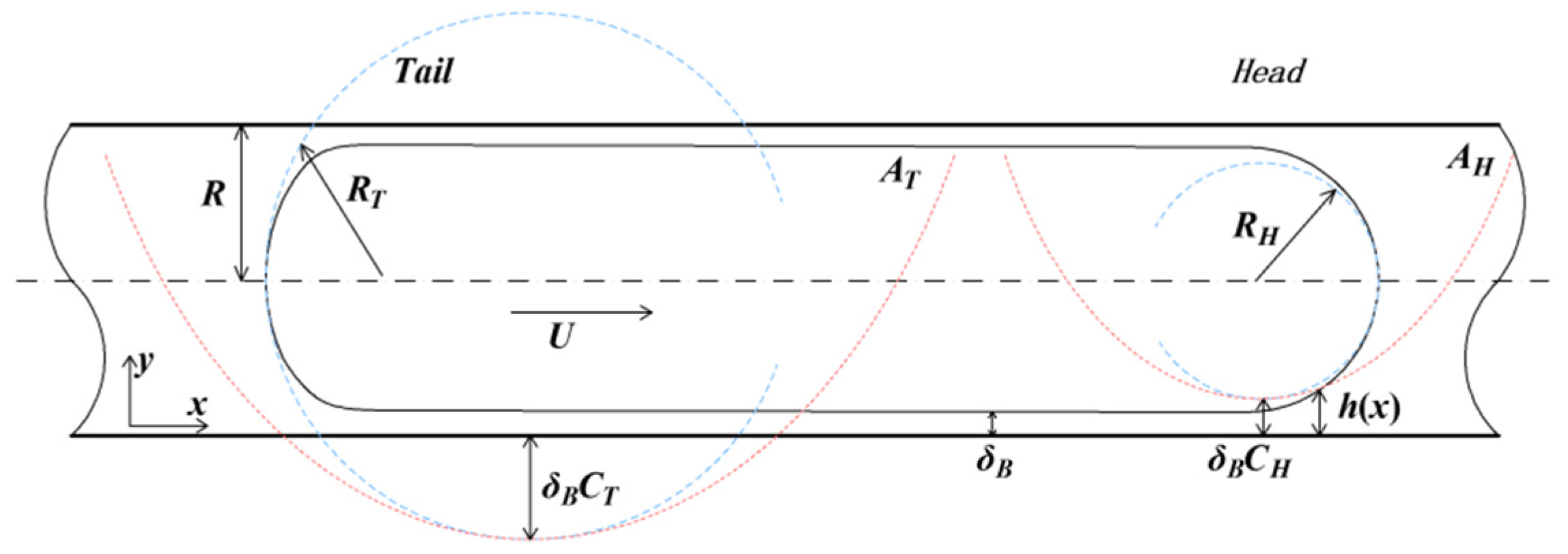
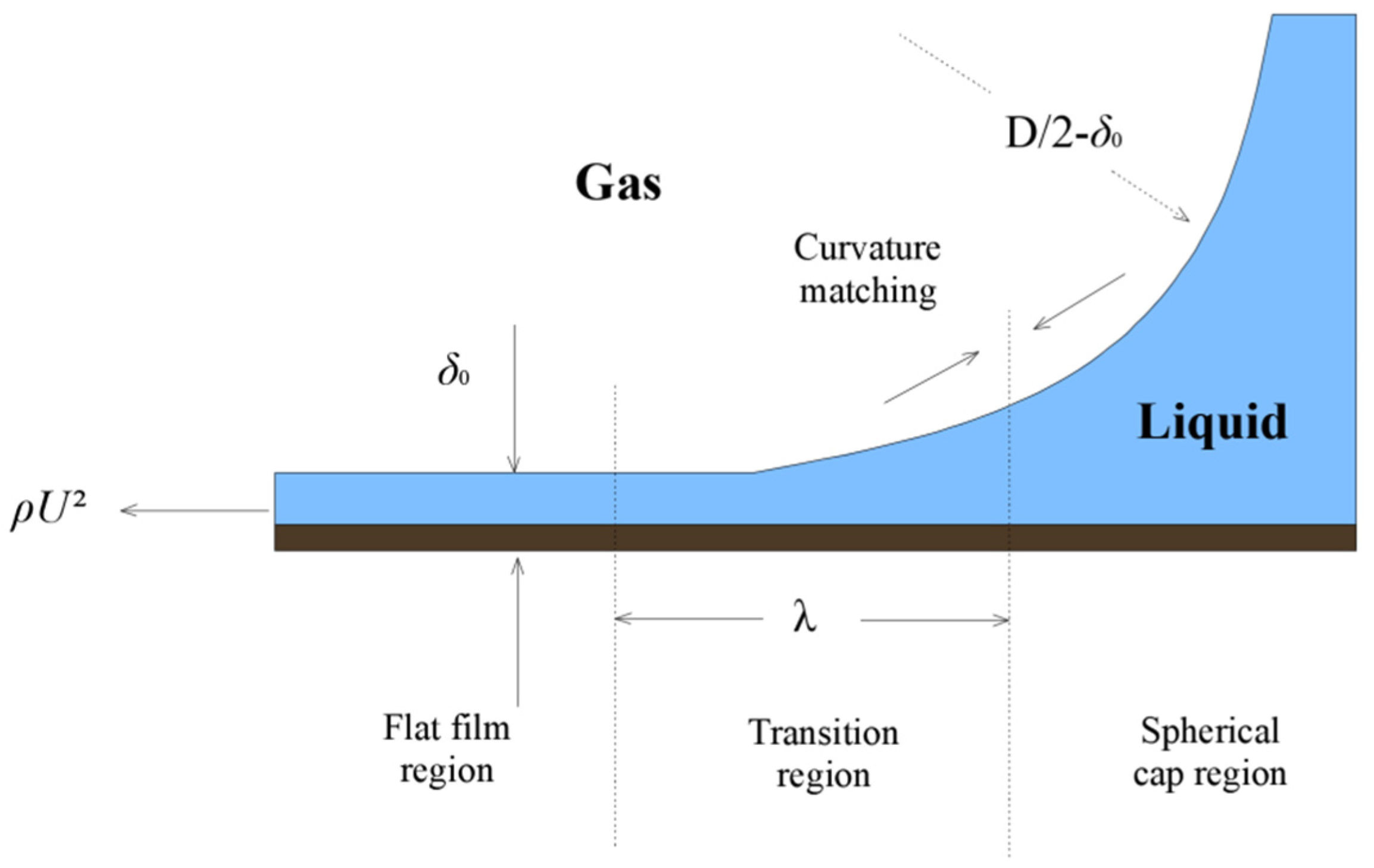
In a cylindrical pipe formed by a gas–liquid two-phase fluid mixture in a slug flow, the bubble can be approximated as a cylinder with two nearly hemispherical caps. As shown in Figure 4, the middle section of the bubble can be approximated as consisting of a cylindrical cavity and a uniform thickness liquid film wrapped around the outside. The two ends of the bubble consist of a three-dimensional surface with a very complex shape and a nearly spherical surface at the top, as shown in Figure 5. The slug bubble that can exist stably in the circular tube has a length several times the diameter of the circular tube, while the gas flow rate is mainly calculated based on the main body of the bubble. Therefore, the actual shape of the bubble ends has little effect on the calculation of the total volume flow rate of the gas.

Due to the random nature of the gas–liquid two-phase flow, the lengths of both bubbles and liquid slugs were not identical. It was assumed that all bubbles had the same length and were multiples of the diameter of the circular tube. Similarly, it was assumed that all liquid slugs were of the same length. The object of calculation and analysis was a cell consisting of a bubble and a slug. Based on the theory of multiphase media, a mathematical model of slug flow in a circular tube section in axisymmetric form was established. Firstly, it can be assumed that the computational domain of a single fluid based on the mass conservation equation can be obtained as the continuity equation in column coordinates (x, r, θ) [28]

$$\frac{\partial \rho }{\partial t}+\frac{\partial \left(\rho u_{r}r\right)}{r\partial r}+\frac{\partial \left(\rho u_{\theta }\right)}{r\partial \theta }+\frac{\partial \left(\rho u_x\right)}{\partial x}=0$$

(11)

The Navier–Stokes equation projected onto the x-axis in the column coordinate system can be written in the following form

$$\rho \left(\frac{\partial u_x}{\partial t}+u_r\frac{\partial u_x}{\partial r}+\frac{u_{\theta }}{r}\frac{\partial u_x}{\partial \theta }+u_x\frac{\partial u_x}{\partial x}\right)=-\frac{\partial }{\partial x}\left(p-\rho g_{x}x\right)+\mu {\nabla }^2{u}_x$$

(12)

Equations (11) and (12) describe the flow of bubbles and liquid films. Since the liquid was incompressible and the volume of the bubble remained almost constant, it can be assumed that the density ρ of each phase was constant. Since $u_{\theta }=0$ and $u_r=0$ characterized the axisymmetric model, $\frac{\partial u_x}{\partial x}=0$ can be obtained from Equation (11), and further $\frac{{\partial }^2{u}_x}{\partial x^2}=0$. Therefore, Equation (12) can be simplified to the following form

$${\nu }_j\frac{1}{r}\frac{\partial }{\partial r}\left(r\frac{\partial u_j}{\partial r}\right)=-g_j^{\prime } , j=1, 2$$

(13)

where $u_1$ and $u_2$ denote the velocity components of the continuous phase (liquid film or liquid) and the dispersed phase (bubble or droplet) along the x-axis, respectively, and $g_j^{\prime }$ is the effective gravitational acceleration component of the gravity and pressure gradient acting on the dispersed or continuous phase along the x-axis.

The conventional view is that the low viscosity properties of the gas result in minimal shear stress on the bubble surface, which can be neglected in calculations. However, the effect of shear stress on bubbles and droplets in slug flows can be substantial due to the small transverse dimensions of bubbles and liquid films in small-diameter circular tubes. At the axis of the circular tube (r = 0), the shear stress in the bubble is zero.

$${\tau }_2={\mu }_2\left(\frac{\partial u_x}{\partial r}+\frac{\partial u_r}{\partial x}\right)=0$$

(14)

This equation can be combined with Equation (11) to obtain

$${\left.\frac{\partial u_2}{\partial r}\right|}_{r=0}=0$$

(15)

Meanwhile, the tube wall obeys the no-slip boundary condition at r = R

$${\left.u_1\right|}_{r=R}=0$$

(16)

At the gas–liquid interface ($r=R_B=R-\delta$), the mixed boundary condition is used to characterize the continuity of the velocity and shear stress distribution in the system,

$${\left.u_1\right|}_{r=R_B}={\left.u_2\right|}_{r=R_B}$$

(17)

$${\left.{\tau }_1\right|}_{r=R_B}={\left.{\tau }_2\right|}_{r=R_B}$$

(18)

The above equation can be further written as

$${\left.{\tau }_1\right|}_{r=R_B}={\left.{\mu }_1\frac{\partial u_1}{\partial r}\right|}_{r=R_B}={\left.{\tau }_2\right|}_{r=R_B}={\left.{\mu }_2\frac{\partial u_2}{\partial r}\right|}_{r=R_B}$$

(19)

Double integration of the gas–liquid phase in Equation (13) yields

$$\frac{\partial u_i}{\partial r}=-\frac{g_i^{\prime }}{2{\nu }_i}r+\frac{C_{1i}}{r}, i=1, 2$$

(20)

$$u_i=-\frac{g_i^{\prime }}{2{\nu }_i}\frac{r^2}{2}+C_{1i}\ln r+C_{2i}, i=1, 2$$

(21)

where the integration constants $C_{1i}$ and $C_{2i}$ can be calculated by the boundary conditions (Equations (16)–(19)). The velocity and stress distribution of the continuous phase (liquid film) in the velocity distribution of each phase of the mixture is shown below

$$u_1\left(r\right)=C_1^{\prime }\left(R^2-r^2\right)-C_1\ln \left(\frac{R}{r}\right)$$

(22)

$${\tau }_1\left(r\right)={\mu }_1\frac{\partial u_1}{\partial r}={\mu }_1\left(-2C_1^{\prime }r+\frac{C_1}{r}\right)$$

(23)

The velocity and stress distribution in the dispersed phase (bubbles or droplets) are shown below

$$u_2\left(r\right)=C_1^{\prime }\left(R^2-R_B^2\right)+C_2^{\prime }\left(R_B^2-r^2\right)-C_1\ln \left(\frac{R}{R_B}\right)$$

(24)

$${\tau }_2\left(r\right)={\mu }_2\frac{\partial u_2}{\partial r}=-2{\mu }_2{C}_2^{\prime }r$$

(25)

Each parameter in the formula is calculated as follows

$$\left\{\begin{array}{c}{C}_1=\left({\rho }_1-{\rho }_2\right)g_x\frac{R_B^2}{2{\mu }_1}\\ C_1^{\prime }=\frac{g_1^{\prime }}{4{\nu }_1}=\frac{1}{4{\nu }_1}\left(g_x-\frac{1}{{\rho }_1}\frac{\partial p}{\partial x}\right)\\ C_2^{\prime }=\frac{g_1^{\prime }}{4{\nu }_2}=\frac{1}{4{\nu }_2}\left(g_x-\frac{1}{{\rho }_2}\frac{\partial p}{\partial x}\right)\end{array}\right.$$

(26)

The instantaneous flow rate of the liquid in the liquid film can be obtained by integrating Equation (22)

$$\begin{gathered} q_{lf}=2\pi {\int }_{R_B}^R{u}_1\left(r\right)dr \\ =\pi R^2\left(C_1^{\prime }\frac{R^2}{2}-\frac{C_1}{2}\right)-\pi R_B^2\left[C_1^{\prime }\left(R^2-\frac{R_B^2}{2}\right)-C_1\left(\ln \left(\frac{R}{R_B}\right)+\frac{1}{2}\right)\right] \\ =\frac{\pi }{8{\nu }_1}\left(g_x-\frac{1}{{\rho }_1}\frac{\partial p}{\partial x}\right){\left(R^2-R_B^2\right)}^2-\pi C_1\left[\frac{R^2-R_B^2}{2}-R_B^2\ln \left(\frac{R}{R_B}\right)\right] \end{gathered}$$

(27)

The instantaneous flow rate of the gas in the bubble can be found by integrating Equation (24)

$$\begin{gathered} q_G=2\pi {\int }_0^{R_B}{u}_2\left(r\right)dr \\ =\pi R_B^2\left[C_1^{\prime }\left(R^2-R_B^2\right)-C_1\ln \left(\frac{R}{R_B}\right)+C_2^{\prime }\frac{R_B^2}{2}\right] \\ =\frac{\pi }{4}{g}_x\left[\frac{R_B^2\left(R^2-R_B^2\right)}{{\nu }_1}+\frac{R_B^4}{2{\nu }_2}\right]-\frac{\pi }{4}\frac{\partial p}{\partial x}\left[\frac{R_B^2\left(R^2-R_B^2\right)}{{\mu }_1}+\frac{R_B^4}{2{\mu }_2}\right]-\pi C_1{R}_B^2\ln \left(\frac{R}{R_B}\right) \end{gathered}$$

(28)

Thulasidas [29] provided the instantaneous flow rate relationship for a gas–liquid two-phase mixture in a tube during flow based on the assumption that the direction of flow through the liquid film is always opposite to the direction of the bubble velocity

$$q_G=q_{LS}+q_{lf}$$

(29)

The difference is that Aditya extends the assumptions to

$$U_B{A}_B+U_{lf}{A}_{lf}=U_{LS}A$$

(30)

Or

$$q_G+q_{lf}=q_{LS}$$

(31)

The expressions (17)–(19) have the meaning of balanced equations: the left side of its equal sign is the sum of the volume fluxes of each phase entering or leaving the control volume V through the cross-section x = 0, while the right side is the sum of the volume fluxes of each phase entering or leaving the control volume V through the cross-section x = L.

Equation (31) assumes that the flow direction of the film should always be opposite to the flow direction of the bubbles. It is known that the velocity of the bubble is higher than the velocity of the liquid in the slug, i.e., $U_B>U_{LS}$. It can be seen from Equation (30) that, depending on the area of the bubble cross-section, the flow direction of the liquid in the film may be the same as the movement direction of the bubble when the area of the bubble cross-section is small. However, the film flow direction is opposite when the bubble occupies most of the cross-section of the pipe.

After a simple algebraic operation using Equations (27)–(29), the pressure gradient along the bubble axis in the liquid film can be written as

$$\frac{\partial p}{\partial x}=\frac{\left(C_1^{″}-C_2^{″}\right)g_x-q_s}{C_3^{″}}$$

(32)

The following equation can calculate the constants

$$\left\{\begin{array}{c}{C}_1^{″}=\frac{\pi }{8}\left(\frac{R^4-R_B^4}{{\nu }_1}+\frac{R_B^4}{{\nu }_2}\right)\\ C_2^{″}=\frac{\pi }{4}\frac{R_B^2\left(R^2-R_B^2\right)}{{\mu }_1}\left({\rho }_1-{\rho }_2\right)\\ C_3^{″}=\frac{\pi }{8}\left(\frac{R^4-R_B^4}{{\mu }_1}+\frac{R_B^4}{{\mu }_2}\right)\end{array}\right.$$

(33)

However, when the fluid velocity or siphon diameter decreases, the film thickness decreases until it disappears, and the pressure drop of the fluid inside the tube can no longer be calculated using such equations based on the film thickness.

3.2. Mechanism and Calculation for Pressure Drop of Dry Slug Flow

Unlike single-phase flow motion, the mechanical properties of slug flow depend heavily on the bubble-liquid interaction. The mechanical transfer properties of wet slug flow have been discussed when a liquid film is present, while the calculation of dry slug flow is more intuitive.

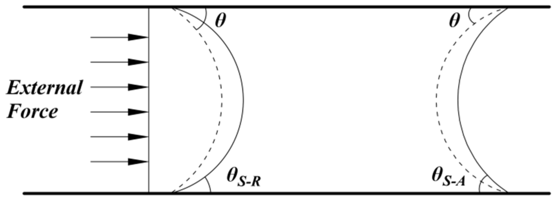
When the bubble is composed of the gas–liquid interface at both ends and the tube wall, instead of only the gas–liquid interface, this flow type can be considered a dry slug flow, while the gas–liquid interface and the tube wall form a gas–liquid–solid three-phase contact line. The most widely used theoretical models regarding the relationship between contact angle and contact line velocity are fluid dynamics [30] and molecular dynamics theory [31]. Among them, the molecular dynamics theory model suggests that the motion of the contact line is determined by the statistical dynamics of collisions between gas, solid, and liquid molecules in the three-phase region [31], as defined by

$$U=2{\kappa }^0\lambda \sinh \left[\frac{\sigma \left(\cos {\theta }_S-\cos {\theta }_D\right){\vartheta }^2}{2k_{B}T}\right]$$

(34)

where ϑ is the average displacement length, $k_B$ is Boltzmann’s constant, h is Planck’s constant, T is temperature; ${\kappa }^0$ is the equilibrium frequency of random displacement of molecules, which can be expressed in terms of the activation energy of the wetting process

$${\kappa }^0=\left(\frac{k_B}{h}\right)\exp \left(-\frac{\Delta E}{N{k}_{B}T}\right)$$

(35)

where N is Avogadro’s constant.

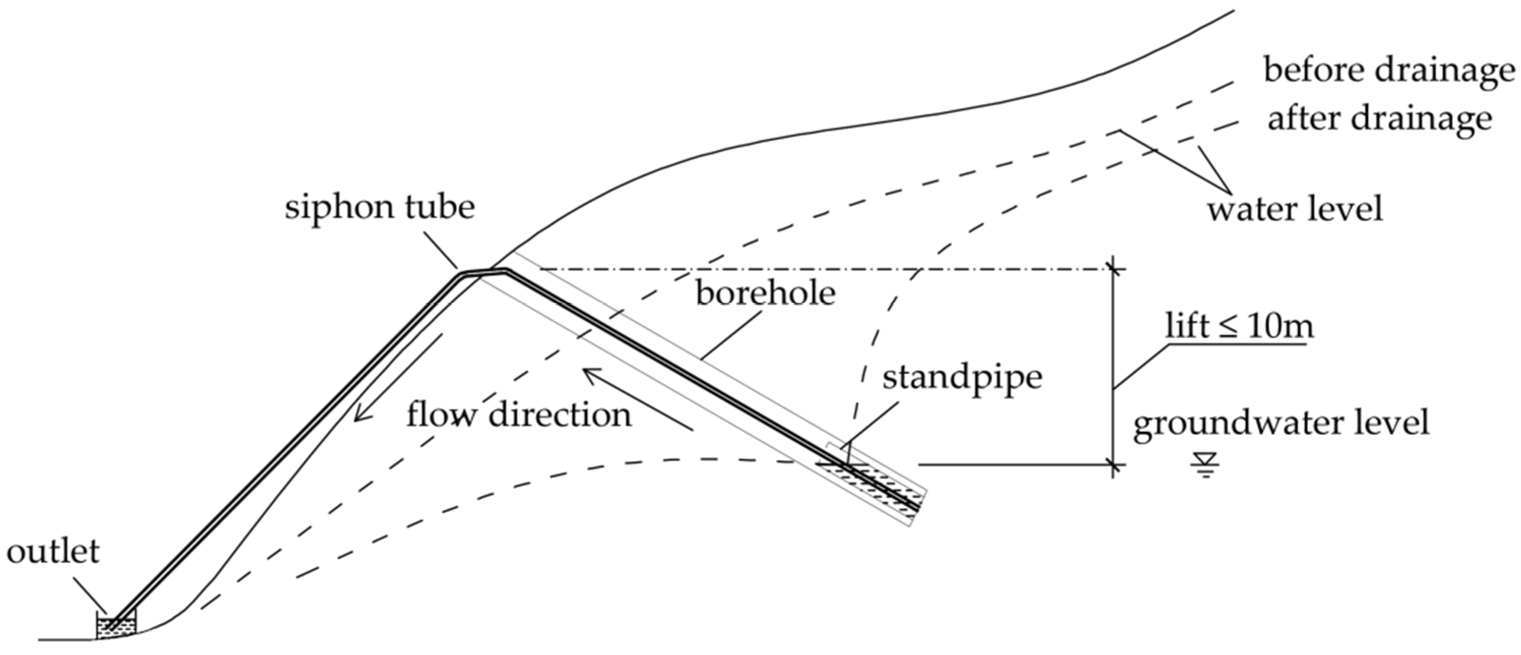
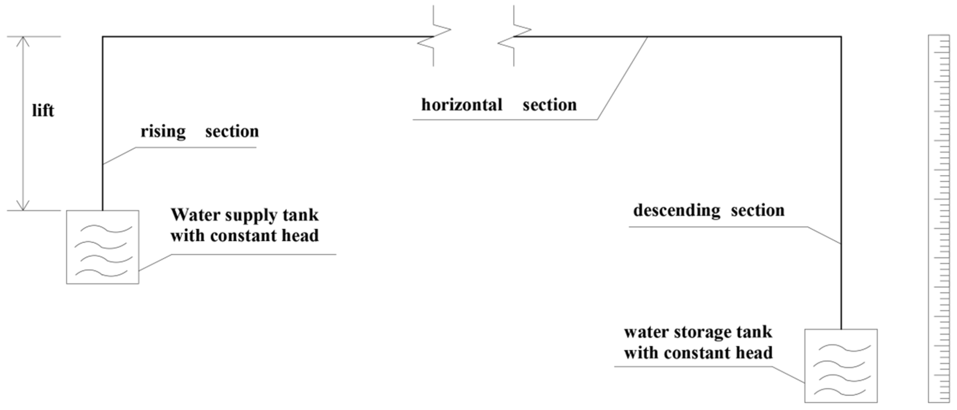
During the siphon drainage process, the fluid in the rising section pushes the fluid in the horizontal section toward the drain. In a millimeter-diameter siphon, the horizontal segment fluid undergoes a discontinuous motion under the action of thrust. Assuming that the fluid does not compress, the forces during the entire motion include fluid thrust, slug bubble interface pressure, resistance along the wall, and negative pressure on the drain side of the slug bubble. Further, the primary energy conversion process of its motion process is gravitational potential energy → kinetic energy → pressure potential energy, → kinetic energy … finally transformed into pressure potential energy, pushing the horizontal segment terminal fluid to vertical segment drop, forming a continuous siphon flow. For siphons in this size range, in the process of resuming siphoning through water level lift, the thrust provided by the lift change is consumed step-by-step by the slug bubble and liquid slug in the horizontal section, plus the resistance effect of the interface between the two ends of the slug bubble and the pipe wall, resulting in a certain degree of reduction in the critical lift that causes siphon restart. A simplified force model of the dry slug flow unit is shown in Figure 6. In this form of flow, the bubbles have the same velocity as the liquid and flow alternately through the pipe without forming a liquid film on the pipe wall. According to the simplified model, it is known that the pressure drop of the slug flow can be divided into three parts, namely, the frictional pressure drop of the bubble and fluid movement and the frictional pressure drop generated by the movement of the gas–liquid–solid three-phase contact line, as shown in Figure 7 for the simplified pressure drop model.

In the dry slug flow mode, the gas, liquid, and solid phases are entirely separated by the gas–liquid interface and moving contact line, and the bubbles have the same velocity as the liquid and flow alternately through the pipe and do not form a liquid film on the pipe wall. Therefore, to satisfy the continuity equation, the velocities of bubbles and slugs should be equal, as shown in the following equation.

$$U_L=U_G=U$$

(36)

The subscripts L and G denote the liquid and gas phases, respectively. In this section, we study the velocity of bubbles and liquid slugs based on the average interfacial velocity of liquid slugs based on the visualized data.

Under experimental conditions, the two-phase flow is dry slug flow when the liquid slug passes through a small diameter channel with hydrophobic properties. According to previous studies, the pressure drop of the two-phase flow consists of the pressure drop of the liquid slug, the bubble, and the moving contact line [32] as follows

$$\Delta P_{TP}=\Delta P_G+\Delta P_L+\Delta P_{MCL}$$

(37)

where ΔP is the pressure drop, the subscripts TP, G, L, and MCL are the two-phase integrated gas phase, liquid phase, and contact line, respectively. As the measured flow velocities at each lift of the 200 m length siphon involved in the test and at the medium and high lift of the 100 m length siphon proved that the siphon flow in the 3~8 mm diameter tube is laminar, the frictional pressure drop of each single phase bubble or liquid slug can be calculated by the following equation

$$\Delta P_G=f_G\frac{L_G}{D}\frac{1}{2}{\rho }_G{u}^2$$

(38)

$$\Delta P_L=f_L\frac{L_L}{D}\frac{1}{2}{\rho }_L{u}^2$$

(39)

The following equation can express the pressure drop of the slug flow

$$\Delta P_{TP}=f_L\frac{L_L}{D}\frac{1}{2}{\rho }_L{u}^2+f_G\frac{L_G}{D}\frac{1}{2}{\rho }_G{u}^2+\Delta P_{MCL}$$

(40)

In addition, pressure loss is also induced when the gas–liquid–solid three-phase contact line moves, i.e., the third term on the right-hand side of the Equation (38). The difference in density and surface tension between different fluids will create a curved interface, and any curved interface between the two phases of the fluid will create a pressure difference that depends on the exact shape of the interface. However, in many cases, the gas–liquid interface can be assumed to be a curved lunar surface described using only the contact angle and the hydraulic diameter. The contact angle depends on the hydrodynamics at the contact line; thus, that part of the pressure drop can be referred to as the contact angle or the pressure drop due to the contact line. The pressure drop at the contact line of the “bubble-liquid slug” cell can be expressed by applying Young’s equation to the contact line

$$\Delta P_{MCL}=-\frac{4{\sigma }_L}{D}\left(\cos {\theta }_A-\cos {\theta }_R\right)$$

(41)

where ${\theta }_A$ and ${\theta }_R$ are the forward and backward contact angles, respectively. Therefore, as long as the forward and backward contact angles differ, a net pressure drop is generated in the contact line. Moreover, the difference between the forward and backward contact angles is caused by two phenomena, i.e., contact angle hysteresis and the effect of contact line velocity on contact angle. Although previous models considered the effect of contact line velocity, the pressure drop caused by contact angle hysteresis was not considered.

Yu et al. [33] proposed that the magnitude of the dynamic contact angle is related to the capillary number Ca, and these correlations have the following form.

$$H=cC{a}^d=\frac{\cos {\theta }_{S-A}-\cos {\theta }_{D-A}}{\cos {\theta }_{\alpha }+1}$$

(42)

where ${\theta }_{S-A}$ and ${\theta }_{D-A}$ are the static advancing contact angle, and dynamic advancing contact angle, respectively, and both c and d are constants. Therefore, the dynamic advancing contact angle can be calculated as

$${\theta }_{D-A}={\cos }^{-1}\left[\cos {\theta }_{S-A}-cC{a}^d\left(\cos {\theta }_{S-A}+1\right)\right]$$

(43)

Regarding the values of c and d, according to Seebergh [34], the way the dynamic contact angle varies and the values of the relevant constants are obtained, as follows Equation

$$H=\left\{\begin{array}{c}4.47C{a}^{0.42} (Ca<1\times {10}^{-3})\\ 2.24C{a}^{0.54} (Ca>1\times {10}^{-3})\end{array}\right.$$

(44)

Although the model does not contain any empirical parameters, it only applies to the forward contact line velocity solution, i.e., the dynamic forward contact angle. In order to be able to apply the above equation to the dynamic backward contact angle, in previous work on the model calculation, it was assumed that the difference between the static and dynamic backward contact angle is the same as the difference between the static and dynamic forward contact angle. Thus, the dynamic backward contact angle can be calculated according to the following equation

$${\theta }_{S-R}-{\theta }_{D-R}={\theta }_{D-A}-{\theta }_{S-A}$$

(45)

where ${\theta }_{S-R}$ and ${\theta }_{D-R}$ are the static and dynamic backward contact angles, and ${\theta }_{S-A}$ and ${\theta }_{D-A}$ are the static and dynamic forward contact angles, respectively. According to the above formula, it is known that the larger the flow velocity is, the more significant difference between the static contact angle and dynamic contact angle is; conversely, the smaller it is. Combined with the formula of the critical radius, the calculation results within the application range of this formula show a monotonic decreasing trend with the increase of the contact angle. Therefore, during siphon drainage with a low lift and high flow rate, the end of the liquid slug in the horizontal section of the siphon (corresponding to the head of the slug bubble) is prone to rupture, while the head of the liquid slug is relatively intact, and this phenomenon is also observed in the experiment.

The relationships between the four dynamic static contact angles were obtained from Equation (42) to Equation (45) can be further combined with experimental correlations. First, to eliminate the empirical parameters in the molecular dynamics equations, the independent variables of hyperbolic sine are assumed to be minor, and then the hyperbolic sine function is substituted into its Taylor expansion to reduce Equation (35) to a linear equation

$$U=\frac{{\kappa }^0{\vartheta }^3\sigma \left(\cos {\theta }_S-\cos {\theta }_D\right)}{k_{B}T}$$

(46)

Using Equations (35) and (45) to find U, respectively, and joint, the same equation can be written for the backward contact angle (i.e., −U) to obtain the relationship equation for the contact angle, respectively.

$$\cos {\theta }_{S-R}-\cos {\theta }_{D-R}=\cos {\theta }_{D-A}-\cos {\theta }_{S-A}$$

(47)

The single contact line pressure drop is solved by substituting the dynamic contact angle correlation Equation (44) into Equation (47) and then substituting the resulting dynamic forward and backward contact angles into Equation (41), which obtains the contact line pressure drop associated with the capillary number.

Thus, with the pipe material and fluid type determined, the pressure drop of the moving contact line is then determined by the speed and number of its movements. The slug frequency is the number of fluid slugs that flow through a specific pipe location during a specific time interval. The primary defining equation for slug frequency is

$$f=\frac{U_B}{L_B+L_{LS}}=\frac{U_B}{L_{unit}}$$

(48)

Heywood [35] obtained an improved formula for calculating the slug frequency

$$f=0.0434{\left[\frac{U_{spL}}{U_{LS}}\left(\frac{2.02}{D}+F{r}_S\right)\right]}^{1.02}$$

(49)

where $F{r}_S=\frac{U_{LS}^2}{gD}$.

3.3. Improved Calculation Method for Siphon Flow Rate with Long Horizontal Pipe Sections

The standard siphon velocity calculation is based on Bernoulli’s equation,

$$v=\sqrt{\frac{2g\Delta H}{1+\lambda \frac{l}{D}+\Sigma \zeta }}$$

(50)

which is based on the assumption of continuous single-phase flow and shows that the siphon velocity was influenced by frictional resistance, including along-stream and local lift losses. The effect of lift and height difference on the selection of siphon velocity parameters was further demonstrated by Mei’s study [36], but only a semi-empirical solution was given without a more detailed explanation of the mechanism. The different force transfer characteristics of the fluid in the siphon were analyzed separately by setting the apex of the siphon as the critical analysis plane by Zheng [37]. Different calculation lengths were selected according to the acceleration direction of fluid motion around the critical analysis surface, and smaller values were taken in the results to control the calculation error between 3% and 19%.

Although the calculation errors were significantly reduced, the research focused on the flow velocity calculation of “straight-up- straight-down” siphon drainage systems. Although in long or short siphon systems with a high lift, the fluid will precipitate much air due to the reduction of air pressure. However, in a siphon with a long horizontal section, the effect of frictional resistance from air precipitation increases with the length of the top horizontal section. Therefore, it is urgent and necessary to study the mechanism of siphon flow velocity in siphons with extended horizontal sections and to calculate it accurately in engineering practice.

In his study of short pipe siphoning, Zheng found that the magnitude of the fluid thrust at the top of the siphon plays a crucial role in how the flow velocity is calculated. That is, the ability to maintain continuous flow when the fluid moves to the highest position determines Bernoulli’s equation’s scope of application. However, long horizontal siphons have more complex and stochastic fluid motion than short siphons and have different velocity loss characteristics. For short siphons, the critical analysis surface can be intuitively chosen from the highest point of the siphon based on the energy loss characteristics, but for long horizontal siphons, the fluid will be in a state of continuous energy loss at its highest horizontal position. Therefore, in the process of calculating the siphon flow velocity in the long horizontal section, although the process of air pressure change in the rising section is similar to that in the short tube, the interaction between the fluid and the tube wall in the horizontal section has a considerable effect on the change of flow velocity. Therefore, to extend the formula of siphon flow velocity to the operating mode of long siphons, the analytical calculation of the siphon drainage velocity for the horizontal section should be added to the original formula of segmental integration. Therefore, the siphon velocity loss in the “horizontal section” should be added to the siphon velocity equation considering the effect of the long horizontal section. Based on the above reasoning, and assuming that the siphoned fluid in the horizontal section is a segmental slug flow, i.e., a cross-section at any location with a single-phase composition, this simplifies the computational model to simulate the movement of a homogeneous fluid in the pipe. Similarly, to simulate the most unfavorable state, the calculated length of the horizontal section of the siphon is taken to be the entire length of the horizontal section, as follows.

$$\left\{\begin{array}{c}{P}_{\mathit{veri}}=\rho g\left(h_{\mathit{max}}-\frac{v_{\mathit{ver}0}^2}{2g}-{\sum }_{i=1}^i\left(\frac{v_{\mathit{veri}-1}^2{\lambda }_{i-1}{l}_i}{d}+v_{\mathit{veri}-1}^2{\zeta }_{\mathit{veri}}+l_i\right)\right)\\ v_{\mathit{veri}}=v_{\mathit{ver}0}\frac{H_a\left(P_{\mathit{atm}}-P_{\mathit{veri}}\right)RT+P_{\mathit{veri}}}{P_{\mathit{veri}}},\mathit{for}0<{\sum }_{i=1}^i{l}_i<l_{\mathit{ver}};\\ P_{\mathit{horii}}=\rho g\left(h_{\mathit{atm}}-\frac{v_{\mathit{ver}0}^2}{2g}-{\sum }_{i=1}^i\left(\frac{v_{\mathit{horii}-1}^2{\lambda }_{i-1}{l}_i}{d}+v_{\mathit{horii}-1}^2{\zeta }_{\mathit{upi}}+h_i\right)\right)\\ v_{\mathit{horii}}=v_{\mathit{ver}0}\frac{H_a\left(P_{\mathit{top}}-P_i\right)RT+P_i}{P_i},\mathit{for}{l}_{\mathit{ver}}<{\sum }_{i=1}^i{l}_i\le L_{\mathit{ver}+\mathit{hori}}\end{array}\right.$$

(51)

The calculation of siphon drainage with a long horizontal section can be divided into two parts: the vertical upward section (whose main feature is the decrease in air pressure with increasing height) and the horizontal section (whose main feature is the accumulation of losses along the range). In the vertical upward section of the siphon, the air pressure increases with the height of the position and a “parabolic” type decline occurs, the fluid kinetic energy is converted to gravitational potential energy, and the fluid moves from acceleration to deceleration, but still maintains a significant flow rate. When the fluid moves to the horizontal section, the air pressure value inside shows a state of height, while the change in air pressure is significantly reduced. Based on this, in the fluid motion formula, if we continue to use the calculation of the vertical section of the air pressure, then the value of $P_{hori}$ will continue to decrease, which is not in line with the actual situation. Therefore, to simplify the calculation, the air pressure at the initial position of the horizontal section was approximated by taking the air pressure at the top of the vertical section. Take $P_{hori}=P_{top}$, where $P_{top}$ is a constant value approximately equal to the air pressure at the top of the vertical section, as shown in Equation (51).

In this study, since there was no applied pressure throughout, the air pressure fluctuation inside the tube did not exceed two times the atmospheric pressure, so the air could be precipitated by default with the liquid out of the siphon and no longer dissolved in water. Therefore, when calculating the void ratio and the total length of the air slug, the descending section length of the tube should be included in the calculation of the equation. Therefore, $P_i$ in Equation (51) can be expressed as

$$\Delta P_{hori}=P_{horii}-P_{horii-1}=\Delta P_L+\Delta P_G+\Delta P_{MCL}$$

(52)

Before starting the calculation, some known data need to be given. The input data include the diameter of the circular tube D; the physical properties of each phase ${\rho }_1$, ${\rho }_2$, ${\mu }_1$, ${\mu }_2$, $\sigma$; and the projection of gravitational acceleration in the flow direction $g_x$. The calculation algorithm is described as follows, and the calculation flow chart is given in Figure 8.

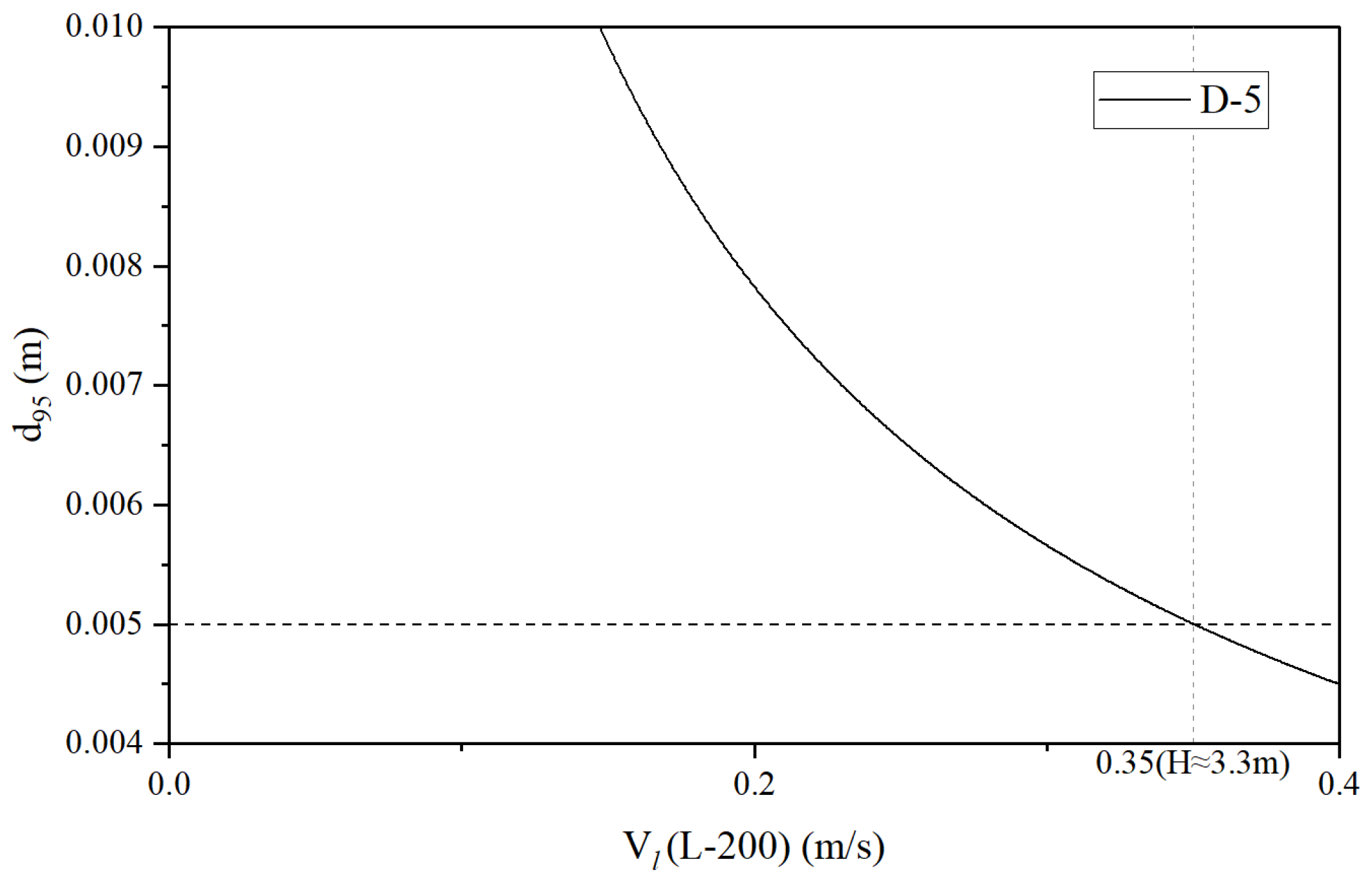
First, we calculated the value of the siphon flow rate in the ideal state without considering air release by using the whole tube as the calculation segment, assigned it to the initial value of the flow rate, and calculated the instantaneous flow rate at the corresponding position according to Equation (51) combined with the change of air pressure occurring in the tube with height up to the horizontal segment. When the iteration proceeds to the horizontal section, a determination of the type of dry or wet slug flow is required. It can be seen that the pressure drop at both ends of the bubble decreased sharply when the capillary number was less than ${10}^{-3}$ from Figure 3 as well as Equation (44). Therefore, to simplify the calculation, the wet slug flow or dry slug flow can be judged according to whether the Ca is greater than ${10}^{-3}$.

When Ca > ${10}^{-3}$, it can be judged as a wet slug flow, and the mathematical models given in Equations (26)–(32) were used to calculate the velocity of each gas–liquid phase, the volume fraction of the gas, and the length of the bubble slug when the bubble size is known. The calculated flow velocity was used as the liquid velocity, i.e., $U_{LS}=v_{hori}$, and the equation proposed by Thulasidas [18] was used to determine the initial approximation of the bubble velocity

$$U_B^0\approx 2.27U_{LS}+0.361{\left(gd\right)}^{0.5}$$

(53)

Then, the capillary number was calculated by using the bubble velocity, and the liquid film thickness δ was determined using $\frac{{\delta }_0}{R}=\frac{1.34C{a}^{\frac{2}{3}}}{1+1.34\times 2.5C{a}^{\frac{2}{3}}}$ [38]. The pressure gradient could be calculated after n iterations of Equations (31) and (32), while the gas flow rate in the bubble, the liquid flow rate in the liquid film, and the bubble motion velocity could be obtained after n iterations of Equations (26) and (27). The relative error $\psi =\frac{2\left(\left|q_{LS}-q_B\right|-\left|q_{lf}\right|\right)}{\left(\left|q_{LS}-q_B\right|+\left|q_{lf}\right|\right)}$ can be used to compare the liquid flow rate in the film and the calculated error ϖ specified value can be used to decide whether to terminate the calculation (when ψ ≤ ϖ) or return to re-substitute the calculated capillary number and repeat the step (when ψ > ϖ).

When Ca < 0.001, it can be judged as dry slug flow. Take the calculated flow velocity as the gas–liquid two-phase velocity $U_{LS}=v_{hori}$, and calculate the moving friction loss of the gas–liquid–solid three-phase contact line according to Equation (41). The value of the slug frequency in the tube at the corresponding flow rate was obtained by Equation (49). In addition, the air pressure, gas precipitation, gas motion velocity, and liquid motion velocity in the tube after n iterations were determined using Equation (52). Comparing the values of the selected parameters, i.e., $\varphi =\frac{\left|U_{LS}-U_B\right|}{\left|U_{LS}+U_B\right|}$, the specified value of the calculation error Δ determines whether to terminate the calculation (when $\varphi \le \Delta$) or to return and repeat the previous ones.

4. Experimental Setup and Scheme

The siphon drainage experimental setup, as shown in Figure 9, was used to validate the proposed calculation method. The experimental setup is a full-scale model and the pipe is made of polyurethane (PU). Thirty-six experiments were performed, and the schemes are given in

Table 1. Experimental schemes of siphon drainage (T = 25 °C, P_la = 100.53 kPa).

No.	D/mm	Lhori/m	Hlift/m
1~4	4	0	3, 4, 5, 6
5~6	4	0	7, 8
7~12	4	80, 160	3, 4, 5
13~18	4	80, 160	6, 7, 8
19~22	5	0	3, 4, 5, 6
23~24	5	0	7, 8
25~32	5	100, 160	3, 4, 5, 6
33~36	5	100, 160	7, 8

, where $D$ represents the diameter of siphon pipe, $L_{hori}$ represents the horizontal section length of siphon pipe, and $H$ represents the siphon lift. The flow velocity was measured by weighting the water collected in the water storage tank for a period. It should be noted that a single-phase flowmeter does not work well in these experiments since the flow pattern is multi-phase.

5. Discussions

According to the improved flow rate calculation method, the values of siphon flow rates for different lengths of 4 mm and 5 mm diameter siphons obtained by iterative calculation based on MATLAB programming are shown in Figure 10. In the legend, “H-No.” is the numerical simulation lift condition; “TH” refers to the test lift.

The results in Figure 10a show that (1) for Experiment Schemes 1–4, the calculated values from Equation (50) and Zheng’s theory are close to the experimental measurements; (2) for Schemes 5–12, the calculated values from the two formulae have significant errors, yet the values from the improved method in this paper are still closed to the experimental measurements; (3) for Schemes 13–18, the errors between the calculated values from the improved method in this paper and the experimental measurements are less than 5%. The traditional siphon calculation theory can predict the short pipe-siphon flow velocity relatively well for smaller lifts. However, for higher lifts, its flow velocity calculation differs from the actual value by about 26%, which is improved in the calculation of Zheng’s theoretical equation. However, Zheng’s formula is also limited to improving the accuracy of flow velocity calculations for short pipe siphons at high-lift conditions. In the case of long siphons, especially with extended horizontal sections of discharge conditions, if the formula continues to be used, the error between the calculated and the experimental results is about 12%, and the error value exceeds the safety limit used for production calculations. Figure 10b shows that the calculated results obtained by the improved method still agree well with the experimental measurements. For the siphon with the long horizontal section, the fitting formula in this study solved this problem relatively well.

When the calculation program initially set the calculation conditions according to the actual horizontal section length of the test, the error rate between the program calculation results and the test results appeared to increase exponentially, which was caused by the over-selection of the calculated pipe length of the horizontal section. This is because in the siphon system the highest horizontal position has a certain degree of “negative pressure”. That is, the air pressure at this position is much smaller than the local atmospheric pressure. For this reason, the reduction in air solubility caused by the reduction in air pressure is significantly magnified in the horizontal section of a siphon with a long horizontal section. In other words, the length of the air bubbles in the long horizontal section is much larger than the length of the air bubbles in the horizontal section of the short tube, which also demonstrates the problem described above regarding the value of the horizontal tube length in the flow rate calculation method. It should be noted that in the process of calculating the siphon flow velocity in the long horizontal section, although the process of air pressure change in the rising section is similar to that in the short tube, the interaction between the fluid and the tube wall in the horizontal section has a considerable effect on the change of flow velocity. When the horizontal section length reduction is not considered, the loss length of the horizontal section of the siphon will gradually decrease as the lift increases, thus leading to an increasing error between the test results and the calculated results, i.e., the calculated results are negligible. When the moving contact line pressure drop is introduced, the error in the calculation equation can be effectively corrected. The siphon limit can be predicted by comparing the calculated flow rate with the minimum limit value at different lifts.

6. Conclusions

The existing classical equations for siphon flow velocity are not applicable to siphon systems with extended horizontal sections because the dominant flow form in siphons is slug flow. Therefore, this study used theoretical analysis, numerical simulation, and experimental validation to explore the final performance of siphon flow velocity for different pipe diameters and lengths of long-distance siphon drainage. As a result, the following insights were obtained: (1) in the gas–liquid two-phase flow formed by the siphon, two subcategories of segmental slug flow with dry and wet force characteristics were generated due to the influence of pipe diameter and flow velocity; (2) the flow process of dry slug flow is closely related to the dynamic contact angle and the formation of the gas–liquid–solid three-phase moving contact line that causes a significant pressure drop; (3) in the long-distance siphon flow calculation process, the calculated length of the horizontal section was reduced to help improve the accuracy of the calculation. By distinguishing and calculating different flow types in the siphon drainage process, an improved method for long pipeline siphon flow velocity based on MATLAB iterative calculation was finally obtained, and its calculation results agreed well with experimental measurements. Furthermore, the error of the calculation results did not exceed 5%, which verifies the reasonableness and effectiveness of the method. Based on the abovementioned understanding, the application of siphon technology in future projects can be flexible in the construction plan by using the improved calculation method to select the pipe length, pipe diameter, and the number of boreholes according to the project drainage needs and topographic constraints. In addition, the following preliminary experience can be gained: the improved calculation method for siphon drainage technology provides a guiding direction for the selection of siphon pipe diameter, i.e., to form a fully developed wet slug flow to ensure no air accumulation in the pipe, and to avoid forming a dry slug flow as much as possible to prevent excessive pressure drop.

References

1. Gress, J.C. Device for Draining Soils in Depth. U.S. Patent US4717284A, 5 January 1988. [Google Scholar]
2. Gress, J.C. Device for Regulating the Flow in a Drainage Siphon Tube. U.S. Patent US5035535A, 30 July 1991. [Google Scholar]
3. Shang, Y.; Cai, Y.; Wei, Z.; Pan, P. Siphon drainage method for landslide prevention. J. Eng. Geol. 2015, 23, 706–711. [Google Scholar]
4. Sun, H.-Y.; Pan, P.; Lü, Q.; Wei, Z.-L.; Xie, W.; Zhan, W. A Case Study of a Rainfall-Induced Landslide Involving Weak Interlayer and Its Treatment Using the Siphon Drainage Method. Bull. Eng. Geol. Environ. 2018, 78, 4063–4074. [Google Scholar] [CrossRef]
5. Cai, Y.; Sun, H.; Shang, Y.; Xiong, X. An Investigation of Flow Characteristics in Slope Siphon Drains. J. Zhejiang Univ. Sci. A 2014, 15, 22–30. [Google Scholar] [CrossRef]
6. Sun, H.; Wang, D.; Shang, Y.; Cai, Y.; Wei, Z. An Improved Siphon Drainage Method for Slope Stabilization. J. Mt. Sci. 2019, 16, 701–713. [Google Scholar] [CrossRef]
7. Gupta, R.; Fletcher, D.F.; Haynes, B.S. On the CFD Modelling of Taylor Flow in Microchannels. Chem. Eng. Sci. 2009, 64, 2941–2950. [Google Scholar] [CrossRef]
8. Gupta, R.; Leung, S.S.Y.; Manica, R.; Fletcher, D.F.; Haynes, B.S. Hydrodynamics of Liquid–Liquid Taylor Flow in Microchannels. Chem. Eng. Sci. 2013, 92, 180–189. [Google Scholar] [CrossRef]
9. Talimi, V.; Muzychka, Y.S.; Kocabiyik, S. A Review on Numerical Studies of Slug Flow Hydrodynamics and Heat Transfer in Microtubes and Microchannels. Int. J. Multiph. Flow 2012, 39, 88–104. [Google Scholar] [CrossRef]
10. Bandara, T.; Nguyen, N.-T.; Rosengarten, G. Slug Flow Heat Transfer without Phase Change in Microchannels: A Review. Chem. Eng. Sci. 2015, 126, 283–295. [Google Scholar] [CrossRef]
11. Haase, S.; Yu Murzin, D.; Salmi, T. Review on Hydrodynamics and Mass Transfer in Minichannel Wall Reactors with Gas–Liquid Taylor Flow. Chem. Eng. Res. Des. 2016, 113, 304–329. [Google Scholar] [CrossRef]
12. Ratulowski, J.; Chang, H. Transport of Gas Bubbles in Capillaries. Phys. Fluids A Fluid Dyn. 1989, 1, 1642–1655. [Google Scholar] [CrossRef]
13. Nogueira, S.; Riethmuller, M.L.; Campos, J.B.L.M.; Pinto, A.M.F.R. Flow Patterns in the Wake of a Taylor Bubble Rising through Vertical Columns of Stagnant and Flowing Newtonian Liquids: An Experimental Study. Chem. Eng. Sci. 2006, 61, 7199–7212. [Google Scholar] [CrossRef]
14. Nogueira, S.; Riethmuler, M.L.; Campos, J.B.L.M.; Pinto, A.M.F.R. Flow in the Nose Region and Annular Film around a Taylor Bubble Rising through Vertical Columns of Stagnant and Flowing Newtonian Liquids. Chem. Eng. Sci. 2006, 61, 845–857. [Google Scholar] [CrossRef]
15. Fabre, J.; Line, A. Modeling of Two-Phase Slug Flow. Annu. Rev. Fluid Mech. 1992, 24, 21–46. [Google Scholar] [CrossRef]
16. Taha, T.; Cui, Z.F. CFD Modelling of Slug Flow in Vertical Tubes. Chem. Eng. Sci. 2006, 61, 676–687. [Google Scholar] [CrossRef]
17. Araújo, J.D.P.; Miranda, J.M.; Pinto, A.M.F.R.; Campos, J.B.L.M. Wide-Ranging Survey on the Laminar Flow of Individual Taylor Bubbles Rising through Stagnant Newtonian Liquids. Int. J. Multiph. Flow 2012, 43, 131–148. [Google Scholar] [CrossRef]
18. Thulasidas, T.C.; Abraham, M.A.; Cerro, R.L. Flow Patterns in Liquid Slugs during Bubble-Train Flow inside Capillaries. Chem. Eng. Sci. 1997, 52, 2947–2962. [Google Scholar] [CrossRef]
19. Zaloha, P.; Kristal, J.; Jiricny, V.; Völkel, N.; Xuereb, C.; Aubin, J. Characteristics of Liquid Slugs in Gas–Liquid Taylor Flow in Microchannels. Chem. Eng. Sci. 2012, 68, 640–649. [Google Scholar] [CrossRef]
20. Rocha, L.; Miranda, J.; Campos, J. Wide Range Simulation Study of Taylor Bubbles in Circular Milli and Microchannels. Micromachines 2017, 8, 154. [Google Scholar] [CrossRef]
21. Suresh, V.; Grotberg, J.B. The Effect of Gravity on Liquid Plug Propagation in a Two-Dimensional Channel. Phys. Fluids 2005, 17, 031507. [Google Scholar] [CrossRef]
22. Khan, N.; Gul, T.; Islam, S.; Khan, I.; Alqahtani, A.; Alshomrani, A. Magnetohydrodynamic Nanoliquid Thin Film Sprayed on a Stretching Cylinder with Heat Transfer. Appl. Sci. 2017, 7, 271. [Google Scholar] [CrossRef]
23. Giavedoni, M.D.; Saita, F.A. The Rear Meniscus of a Long Bubble Steadily Displacing a Newtonian Liquid in a Capillary Tube. Phys. Fluids 1999, 11, 786–794. [Google Scholar] [CrossRef]
24. Heil, M. Finite Reynolds Number Effects in the Bretherton Problem. Phys. Fluids 2001, 13, 2517–2521. [Google Scholar] [CrossRef]
25. Kreutzer, M.T.; Kapteijn, F.; Moulijn, J.A.; Kleijn, C.R.; Heiszwolf, J.J. Inertial and Interfacial Effects on Pressure Drop of Taylor Flow in Capillaries. AIChE J. 2005, 51, 2428–2440. [Google Scholar] [CrossRef]
26. Hinze, J.O. Fundamentals of the Hydrodynamic Mechanism of Splitting in Dispersion Processes. AIChE J. 1955, 1, 289–295. [Google Scholar] [CrossRef]
27. Cherukumudi, A.; Klaseboer, E.; Khan, S.A.; Manica, R. Prediction of the Shape and Pressure Drop of Taylor Bubbles in Circular Tubes. Microfluid. Nanofluidics 2015, 19, 1221–1233. [Google Scholar] [CrossRef]
28. Gupta, R.; Fletcher, D.F.; Haynes, B.S. Taylor Flow in Microchannels: A Review of Experimental and Computational Work. J. Comput. Multiph. Flows 2010, 2, 1–31. [Google Scholar] [CrossRef]
29. Thulasidas, T.C.; Abraham, M.A.; Cerro, R.L. Bubble-Train Flow in Capillaries of Circular and Square Cross Section. Chem. Eng. Sci. 1995, 50, 183–199. [Google Scholar] [CrossRef]
30. Blake, T.D. The Physics of Moving Wetting Lines. J. Colloid Interface Sci. 2006, 299, 1–13. [Google Scholar] [CrossRef]
31. Blake, T.D.; Bracke, M.; Shikhmurzaev, Y.D. Experimental Evidence of Nonlocal Hydrodynamic Influence on the Dynamic Contact Angle. Phys. Fluids 1999, 11, 1995–2007. [Google Scholar] [CrossRef]
32. Lee, C.Y.; Lee, S.Y. Pressure Drop of Two-Phase Dry-Plug Flow in Round Mini-Channels: Effect of Moving Contact Line. Exp. Therm. Fluid Sci. 2010, 34, 1–9. [Google Scholar] [CrossRef]
33. Yu, D.; Choi, C.; Kim, M.H. Pressure Drop and Dynamic Contact Angle of Triple-Line Motion in a Hydrophobic Microchannel. Experimental Therm. Fluid Sci. 2012, 39, 60–70. [Google Scholar] [CrossRef]
34. Seebergh, J.E.; Berg, J.C. Dynamic Wetting in the Low Capillary Number Regime. Chem. Eng. Sci. 1992, 47, 4455–4464. [Google Scholar] [CrossRef]
35. Heywood, N.I.; Richardson, J.F. Slug Flow of Air—Water Mixtures in a Horizontal Pipe: Determination of Liquid Holdup by γ-Ray Absorption. Chem. Eng. Sci. 1979, 34, 17–30. [Google Scholar] [CrossRef]
36. Mei, C.; Liang, X.; Sun, H.; Wu, M. High-Lift Siphon Flow Velocity in a 4-Mm Siphon Hose. J. Zhejiang Univ.-Sci. A 2017, 18, 487–495. [Google Scholar] [CrossRef]
37. Aussillous, P.; Quéré, D. Quick Deposition of a Fluid on the Wall of a Tube. Phys. Fluids 2000, 12, 2367. [Google Scholar] [CrossRef]
38. Zheng, J.; Guo, J.; Wang, J.; Zhang, Y.; Lü, Q.; Sun, H. Calculation of the Flow Velocity of a Siphon. Phys. Fluids 2021, 33, 017105. [Google Scholar] [CrossRef]
Figure 1. Schematic diagram of the inclined pipe-siphon drainage method.
Applsci 12 09660 g001
Figure 2. Bubble d95 curve in 200 m 5 mm siphon pipe.
Applsci 12 09660 g002
Figure 3. Analytical solution curves for the front, the tail, and the total pressure drop of the bubble.
Applsci 12 09660 g003
Figure 4. Schematic diagram of a slug bubble moving with velocity UB in a circular tube.
Applsci 12 09660 g004
Figure 5. The force balance diagram for the bubble’s head, transition, and smooth zone.
Applsci 12 09660 g005
Figure 6. Deformation of the static liquid section slug in a circular tube by force.
Applsci 12 09660 g006
Figure 7. Frictional pressure drop of moving contact line.
Applsci 12 09660 g007
Figure 8. Flowchart of velocity calculation of the siphon with a long horizontal section.
Applsci 12 09660 g008
Figure 9. Diagram of the experimental setup.
Applsci 12 09660 g009
Figure 10. Comparison of MATLAB iterative calculation results with experimental data of siphon flow rate: (a) D-4; (b) D-5.
Applsci 12 09660 g010