Study on Accuracy of CFD Simulations of Wind Environment around High-Rise Buildings: A Comparative Study of k-ε Turbulence Models Based on Polyhedral Meshes and Wind Tunnel Experiments

Abstract

It is important to create a comfortable wind environment around high-rise buildings for outdoor activities. To predict the wind environment, Computational Fluid Dynamics (CFD) has been widely used by designers and engineers. However, the simulation results of different CFD turbulence models might significantly vary. This paper researched the wind environment around a typical high-rise building and verified the accuracy of the CFD simulations based on polyhedral meshes. The differences between the simulation results of the k-ε turbulence models and those of the wind tunnel experiments were compared from the perspectives of wind speed and turbulence energy. The results show that the modified k-ε models could still not perfectly match the wind tunnel experiment results. Specifically, in the low-wind-speed areas, the simulation results of the Realizable Two-Layer K-Epsilon (RTLKE) model were the closest to the experimental results of the wind tunnels, while in the high-wind-speed areas the simulation results of the Standard Two-Layer K-Epsilon (STLKE) model were the closest to the experimental results of the wind tunnels. Therefore, it is recommended that these two k-ε turbulence models are applied under different conditions—the RTLKE model should be used to simulate low-wind areas around high-rise buildings (e.g., defining the size of the static-wind area around high-rise buildings, predicting the diffusion time of pollutants around high-rise buildings, etc.); STLKE should be used to simulate high-wind-speed areas around high-rise buildings (e.g., the high speed wind area around high-rise buildings during a typhoon, the maximum wind speed area around high-rise buildings, etc.). It is expected that findings from this research study supplement some existing high-rise building design guidance.

1. Introduction

Previous research showed that high-rise buildings often have a significant impact on the airflow in their surrounding areas [1,2,3,4,5,6,7], which can be divided into high-wind-speed areas and low-wind-speed areas. High wind speeds can cause some damages, while low wind speeds cannot contribute to the decrease in air pollutants [8,9,10,11]. Moreover, the wind environment around high-rise buildings can impact their energy consumption [12,13]. Therefore, it is necessary and important to predict the wind environment around high-rise buildings before construction. In recent years, Computational Fluid Dynamics (CFD) has been increasingly used in predicting the wind environment, though the accuracy of the calculation results is still under research.

Many scholars have verified the calculation accuracy of different turbulence models based on tetrahedral and hexahedral meshes under different conditions for high-rise buildings [14,15,16,17,18]. For instance, Murakami and Mochida compared the CFD simulation results with wind tunnel experiment results and found that the k-ε model could predict velocity and pressure fields well under fine-mesh conditions [19]. Tan and Li simulated the wind effects on a super high-rise TV tower and found that the Realizable K-Epsilon (RKE) model could come up with more accurate results in terms of mean pressure coefficients and streamlines than the Standard K-Epsilon (SKE) and RNG K-Epsilon models [20]. Behrouzi et al. presented two cases of wind flow around high-rise buildings and concluded that the RNG K-Epsilon model and the RKE model overpredicted the reattachment length behind the buildings [21]. Likewise, other scholars also pointed out the inaccuracy of using revised k–epsilon models in reproducing the weak-wind area and the reattachment length behind the building [22,23,24,25].The Reynolds Stress Model (RSM) with modified inlet atmosphere boundary conditions, as proposed by Zhang et al., was able to better simulate the wind flow around high-rise buildings [26]. Tominaga et al. compared the predicted results using revised K–Epsilon models and Large Eddy Simulation (LES) for a high-rise building and found that the LES showed better performance in predicting mean velocity distributions and turbulence energy distributions [27]. Thordal et al. also found that the LES model showed good performance in predicting the mean surface pressure of high-rise buildings [28,29,30]. Liu et al. evaluated the influence of calculation parameters (e.g., mesh numbers, discretization time step and sampling time, etc.) on simulating the outdoor wind flow around an isolated high-rise building and found that the Detached Eddy Simulation (DES) made a similar prediction of the mean wind velocity field in the lateral side and wake region, while it had less computational cost than the LES [31]. To summarize, the LES model and the DNS model can be more accurate in predicting the airflow, but they require higher computational costs. A range of modified k-ε models can be adopted as a fast solution for many engineering designs and predictions [32,33].

Some scholars explored the accuracy of the CFD simulation results based on different structured mesh generation methods. Du et al. proposed the near-wall mesh generation method to simulate wind environments and evaluated the reliability of this method by comparing the CFD results with the wind tunnel experiment results. The near-wall mesh generation method could provide sufficient near-wall mesh density, while it could not lead to a significant increase in the total amount of meshes and the consequent computational cost [34].

In recent years, with the development of computational technology, the types of mesh calculations based on unstructured mesh generation approaches gradually increased. Nozu et al. assessed the wind pressure distribution and wind force coefficients on the facade of a high-rise building, using the combined model consisting of a Cartesian mesh and an unstructured mesh. The results showed that the wind pressure distribution on the surface could be accurately calculated by using the unstructured mesh system [35]. Blocken and Carmeliet adopted an unstructured mesh with tetrahedral cells in the simulation of complex high-rise residential buildings to evaluate the comfortable outdoor-wind levels for pedestrians [1,36]. The polyhedral mesh has the advantage of achieving better simulation results with relatively fewer meshes. Some scholars analyzed the calculation speed and accuracy of polyhedral meshes and verified the accuracy of the simulation results. For instance, Sosnowski et al. proposed a new method for computational domain discretization based on polyhedral meshes and compared the simulation results generated by three mesh types (i.e., hexahedral, polyhedral, and tetrahedral). It was found that the polyhedral mesh was a reliable choice for computational domain discretization. Moreover, this method could reduce the numerical diffusion of the meshes and the calculation time [37].

Previous research in this field mainly focused on the influence of different turbulence models and parameter settings on the simulation results, and there is no comprehensive study on the accuracy of the simulation results in low- and high-wind-speed areas around high-rise buildings. Some requirements about wind speed were included in the design guidelines for green buildings. For example, “Green Building Evaluation Standard” (GB/T50378-2019) requires that the maximum wind speed is less than 5 m/s at the pedestrian level (1.5 m above the ground) around buildings in winter and that there are no static wind areas in playgrounds in summer [38]. However, the methods of predicting outdoor wind environment and the choices of turbulence models were not suggested in this standard. To fill the gap, this study shed light on the wind flow around a high-rise building using various k-ε turbulence models (e.g., SKE, RKE, etc.) based on polyhedral meshes. The simulation results were cross-compared with the wind tunnel experiment results to verify the accuracy of the simulation under different conditions. It is expected that this study can provide a benchmark for future work and improve the accuracy of predicting the wind environment around a high-rise building.

2. Method

Figure 1 shows the flowchart of this research work.

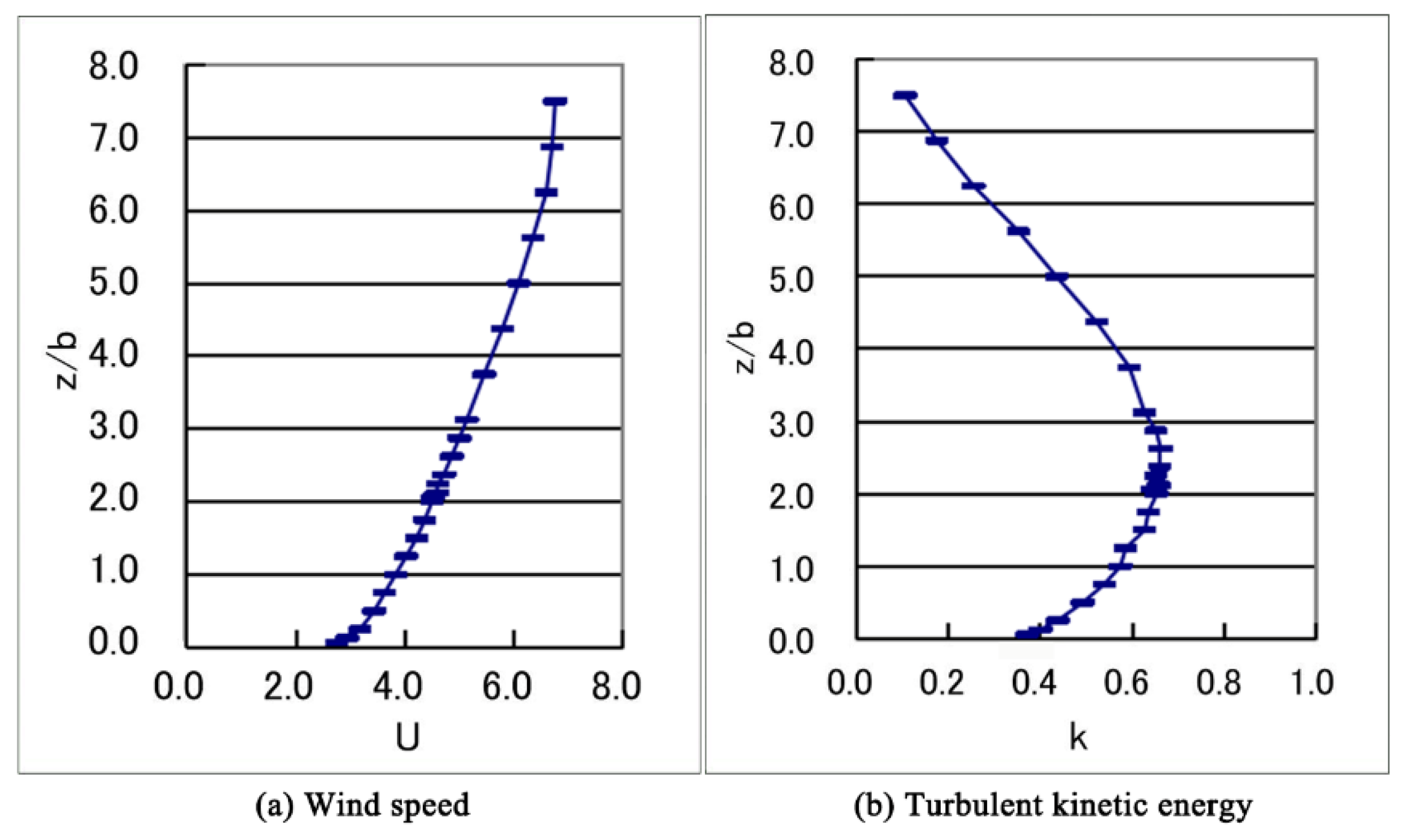
2.1. Outline of Wind Tunnel Experiment

Architectural Institute of Japan (AIJ) has conducted many wind tunnel experiments and summarized the experimental data into a database [16]. This research study selected the case of a single high-rise building from the database as benchmark and compared the numerical simulation results based on the k-ε models and the wind tunnel experiment results from the AIJ database. In the selected case, a high-rise building model with a size of 0.08 m (b) × 0.08 m (d) × 0.16 m (h) was placed in a wind field with a velocity gradient in the vertical direction, and the average wind speed in three dimensions around the model and the average wind speed of the test points on the horizontal plane with heights of 0.125b and 1.25b and the center vertical plane were collected [39,40].

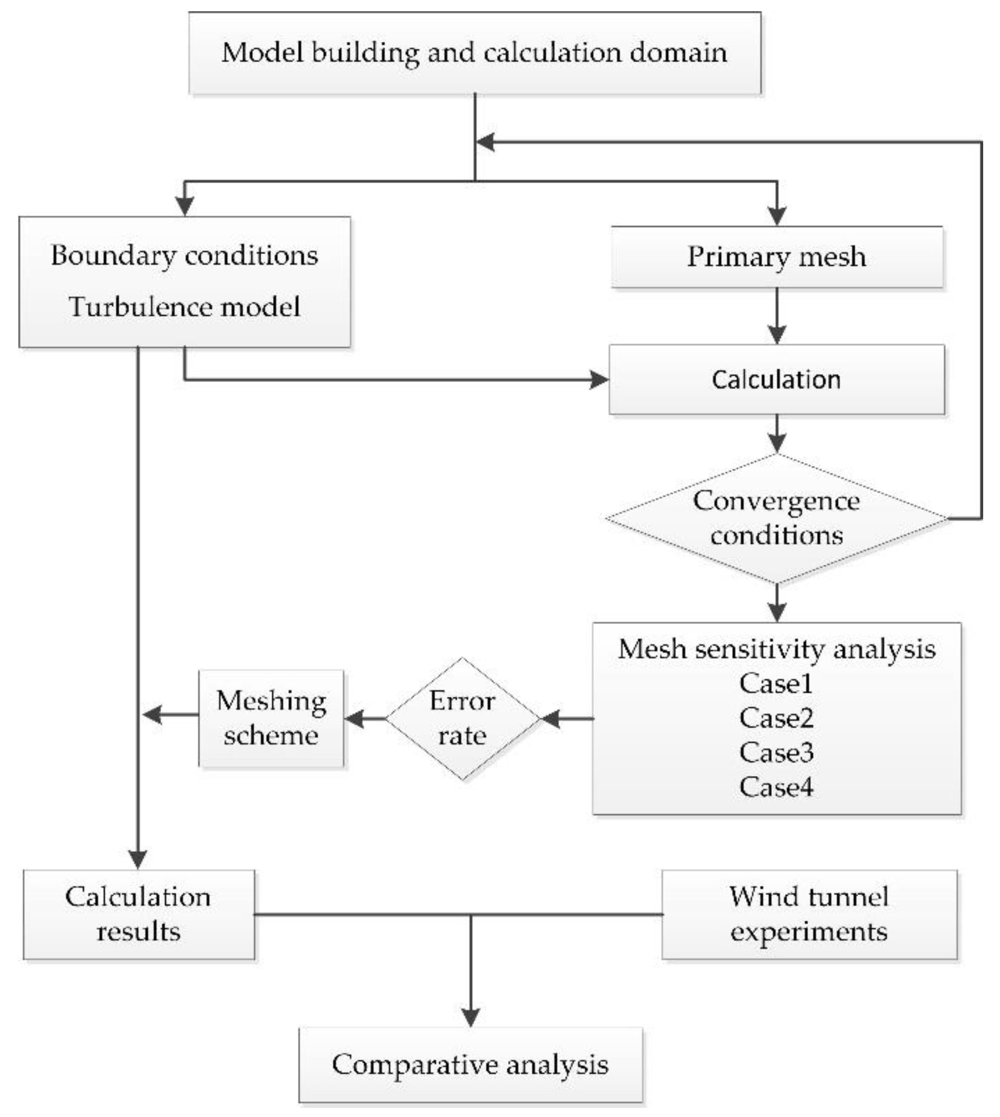
2.2. Numerical Simulations

This research study used Star CCM+ software for numerical simulations. All cases were calculated by the same PC. The parameter settings for the numerical simulations were as detailed below.

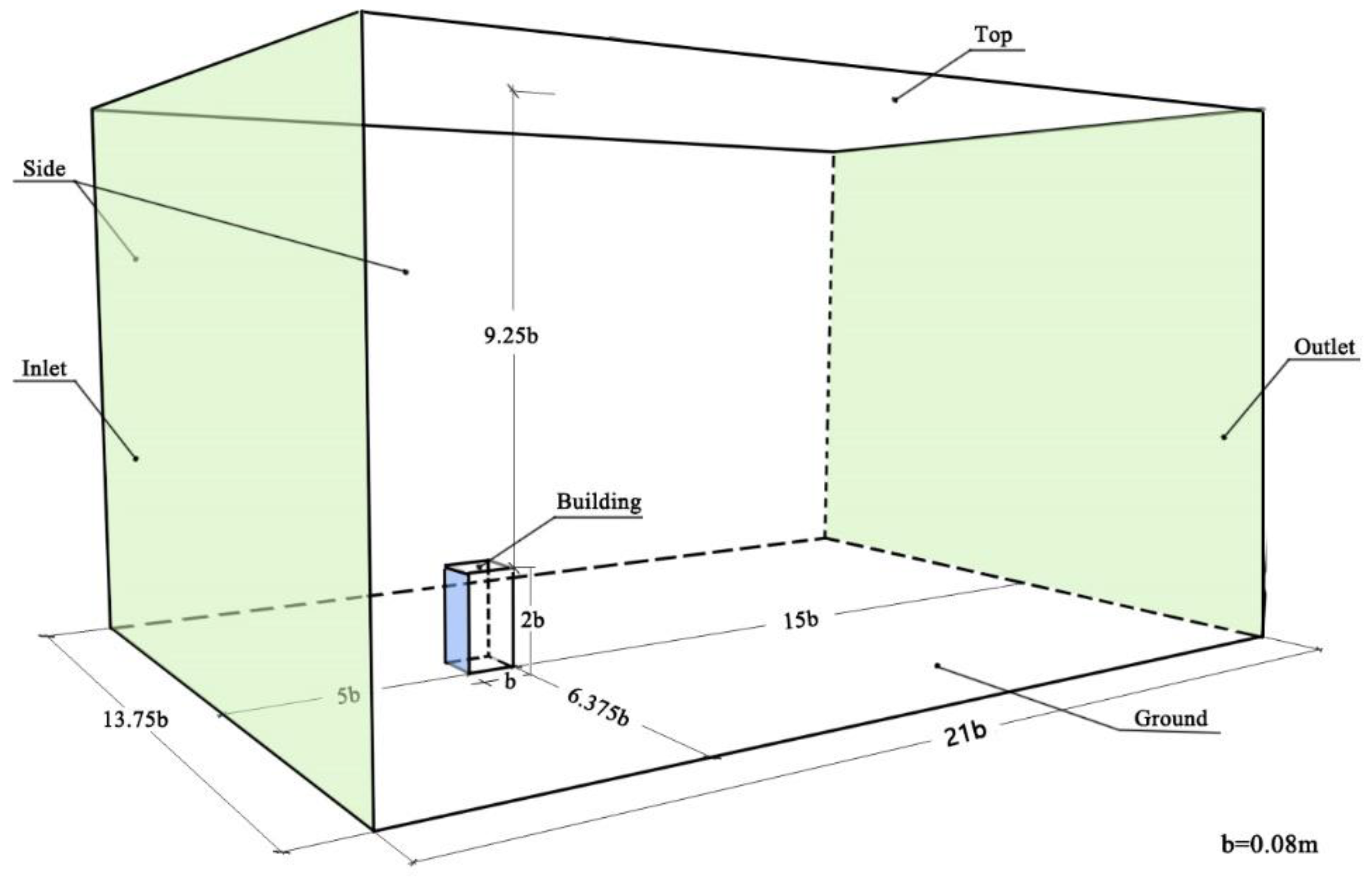
2.2.1. Model Building and Computational Domain

The size of the computational domain was set as 1.68 m × 1.1 m × 0.9 m (Figure 2), referring to previous research [31,39]. The height and width of the domain were the same as those of the wind tunnel experiments. To reduce the influence of inflow profiles, the windward distance was set slightly shorter than that suggested in the AIJ guidelines [31]. The location of the high-rise building model in the domain is shown in Figure 2. The blockage ratio was 1.29%, which was recommended by Frank et al. [41] and Blocken [42].

2.2.2. Boundary Conditions

Inlet boundary: As shown in Figure 3, wind velocity U and turbulent kinetic energy k were set as the same as the values in the wind tunnel experiment. More detailed information can be found from the wind tunnel experiment [39]. Turbulent energy dissipation rate ε could be calculated by Equation (1), where C_μ is a constant with a value of 0.09; k(z) is the turbulent energy, which can be obtained from a wind tunnel experiment or an observation of corresponding surroundings; U(z) is the wind speed at any point in the computational domain; and z is the height of any point in the computational domain [43].

$$\mathsf{\epsilon }\left(z\right)\cong {\mathrm{P}}_k\left(z\right)\cong -\overline{{\mathrm{u}}^{\prime }{\mathrm{w}}^{\prime }}\left(z\right)\frac{\mathit{\text{dU}}\left(z\right)}{dz}\cong {\mathrm{C}}_{\mu }^{\raisebox{1ex}{$1$}\!\left/ \!\raisebox{-1ex}{$2$}\right.}k\left(z\right)\frac{\mathit{\text{dU}}\left(z\right)}{dz}$$

(1)

Outlet boundary: The normal gradients of all variables were set to zero for the outflow [43].

Building-surface boundary and ground boundary: Rough wall conditions and the default parameters of wall roughness in simulation software were used to define the building surface and ground boundary.

Side boundary and top boundary: The smooth wall condition and the default wall treatment in simulation software were used to define the side and top boundaries.

2.2.3. Turbulence Model

The Standard K-Epsilon model was chosen for mesh sensitivity, thereby to determine the appropriate mesh in numerical simulation.

Previous research indicated that the modified k-ε models were suitable for industrial applications in comparison with the LES models and the DNS models. A range of modified k-ε models (e.g., models incorporating wall functions or damping functions) were selected for comparison purposes, including the Standard K-Epsilon (SKE) model [44], the Standard Two-Layer K-Epsilon (STLKE) model [45], the Standard Low-Reynolds Number K-Epsilon (SLRNKE) model [46], the Realizable K-Epsilon (RKE) model [47], the Realizable Two-Layer K-Epsilon (RTLKE) model, the Abe–Kondoh–Nagano Low-Reynolds Number K-Epsilon (AKNKE) model [48], the Elliptic Blending K-Epsilon (EBKE) model [49], and the V2F Low-Reynolds Number K-Epsilon (V2FKE) model [50,51]. The source files of numerical simulation can be find in Supplementary Materials. The simulation results of these models were evaluated against the experimental results based on wind tunnels.

2.2.4. Convergence Conditions

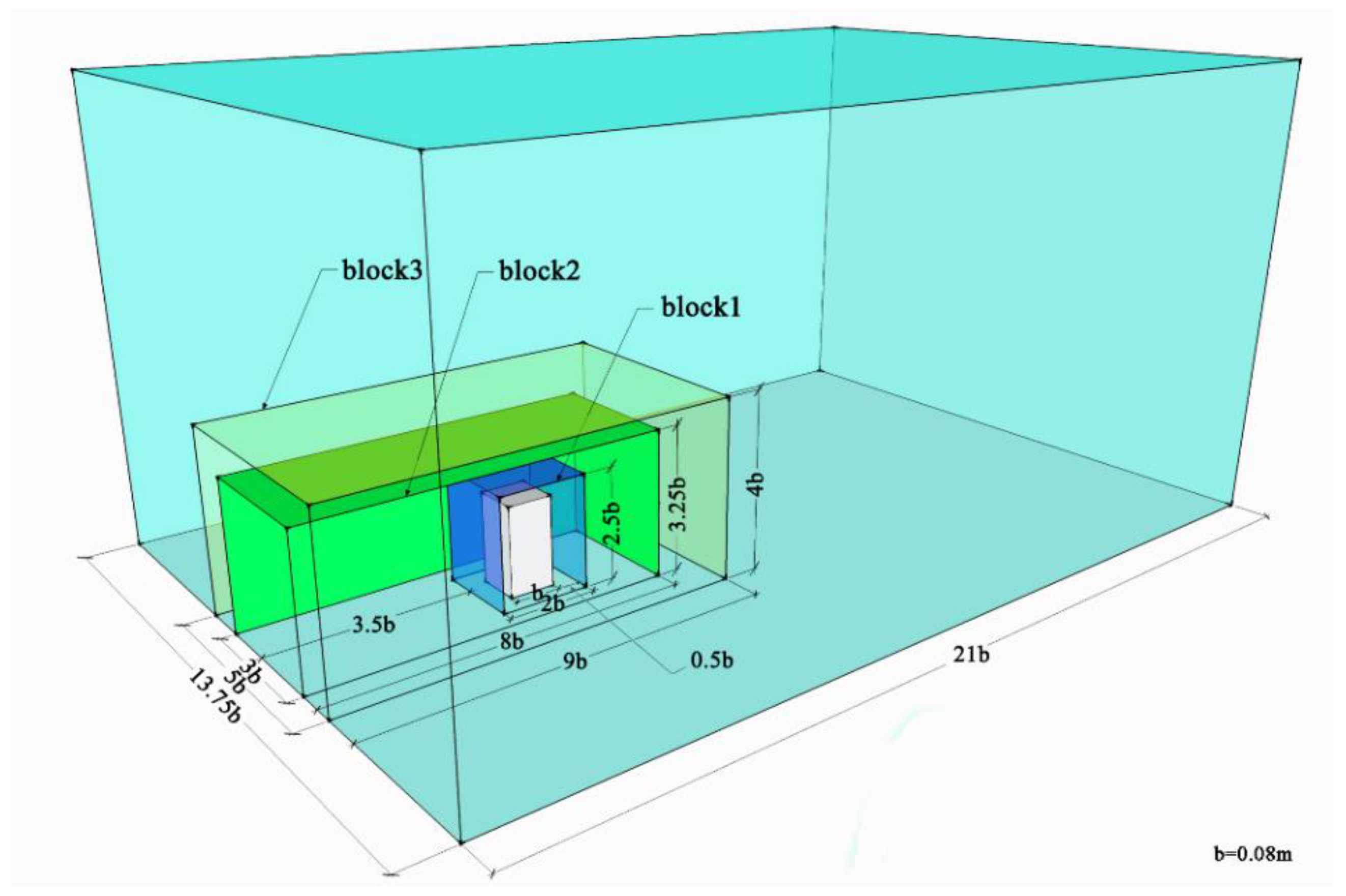
All the calculations were finished until the residuals were less than 10⁻⁴ and the variation values of 50 iterations on specified points were less than 10⁻³ [41,43].

2.2.5. Meshing

A polyhedral mesh is commonly adopted to reduce the calculation time and the numerical diffusion of the mesh (eliminating discretization errors providing a coarse mesh) [37]. In this study, a polyhedral unstructured mesh was used to make a preliminary calculation, where the base mesh size was set to 0.10 m [43]. Base mesh size refers to the reference mesh of the whole computational domain. Besides the custom boundaries and areas, all the surface and volume in the computational domain were divided into the base mesh size. The custom meshes were set with reference to the ratio of the base mesh size [52].

According to the simulation results, the mesh was refined in the areas where the wind speed changed greatly. The mesh close to the building had relatively high density, and the mesh far from the building had relatively low density. Mesh size could be controlled by “Volumetric control” in Star CCM+. Based on the distribution of test points and changes in wind speed in the wind tunnel experiment, three blocks were added around the building, as shown in Figure 4. The sizes of three blocks and the size ratio of the mesh within blocks to the base mesh are shown in

Table 1. Block size and size ratio.

	Length (m)	Width (m)	Height (m)	Block Mesh Size/Base Mesh Size
Block 1	0.16	0.16	0.2	10%
Block 2	0.64	0.24	0.26	15%
Block 3	0.72	0.4	0.32	20%

.

To achieve good computational efficiency, a mesh sensitivity analysis was conducted as described below.

2.3. Mesh Sensitivity Analysis

Four meshing cases were studied for the mesh sensitivity analysis, in which the base mesh sizes gradually became finer, as listed in

Table 2. Mesh and calculation times of 4 cases.

	Base Mesh Size (m)	Architectural Mesh Size (m)	Mesh Numbers of Building Surface	Calculation Time (s)
Case 1	0.10	0.01	977	152
Case 2	0.06	0.006	2869	865
Case 3	0.04	0.004	5944	6235
Case 4	0.02	0.002	23,386	81,154

Legend: Building mesh size refers to the mesh size of the building surface. The ratio of the building mesh size to the base mesh size is 10%.

. Table 2 also shows the mesh numbers and the calculation times for all the cases.

The monitoring points were set in the areas where the wind speeds changed greatly. In total, 66 monitoring points were in the vertical plane at y = 0, and 82 monitoring points were in two horizontal planes at z/b = 0.125 and z/b = 1.25. These monitoring points were distributed around the target building, as shown in Figure 5.

To compare the difference among the above four meshing cases, the error rate proposed by Qin et al. [53] was defined as shown below.

$$\mathrm{Error} \mathrm{Rate}=\frac{\sum \sqrt{{\left(\frac{v_0-v_x}{v_0}\right)}^2}}{n}$$

where v₀ is the value of the finest mesh (Case 4 in Table 2; base mesh size of 0.02 m), v_x is the value of the other mesh (other cases in Table 2; base sizes of 0.1 m, 0.06 m, and 0.04 m), and n is the number of monitoring points.

As shown in Figure 6, the error rates were 16%, 8%, and 6% for Case 1, Case 2, and Case 3, respectively. There was a notable reduction from Case 1 to Case 2, while the error rates for Case 2 and Case 3 were rather close. It was, therefore, concluded that the influence of the mesh size was insignificant once the base mesh size was smaller than 0.06 m. Additionally, the calculation time of Case 3 was nearly 7 times longer than that of Case 2 (Table 2). Considering both calculation time and accuracy, the mesh setting of Case 2 was selected for this study (Figure 7).

3. Results

The inflow wind blocked by high-rise buildings resulted in a separation of the airflow on the lateral sides and the roof of the high-rise building. In this case, the wind speed was relatively faster on the lateral sides and the roof of the building and relatively slower behind the building. This paper focused on the wind environment of the high-wind-speed areas (i.e., the lateral sides and the roof of the high-rise building) and the low-wind-speed area (i.e., the wake region of the high-rise building). Due to the limited test points in the wind tunnel experiment and mesh refinement around the building in the simulations, the contours close to the high-rise building were different from those of the wind tunnel experiment. This was beyond the scope of this research study and requires further studies in future.

3.1. Reattachment Length Comparison

The reattachment lengths [54] on the top of the building (X_R) and behind the building (X_F) are shown in Figure 8 [40]. Different CFD codes or different calculation conditions lead to different simulation results [55].

Table 3. Calculation results of each turbulence model.

	SKE	STLKE	SLRNKE	RKE	RTLKE	AKNKE	EBKE	V2FKE	Wind Tunnel Experiment
XR/b	—	0.33	—	0.38	0.32	0.89	0.37	0.85	0.52
XF/b	2.63	2.38	2.53	3.05	2.65	3.55	3.20	4.35	1.42

lists the relative reattachment lengths on the top of the building (X_R/b) and behind the building (X_F/b) for eight turbulence models and the corresponding wind tunnel experiment. The SKE and SLRNKE models did not show a reattachment on the top of the building, which was inconsistent with the experiment. The X_F/b-value for the V2FKE model was much higher than the value derived from the experiment. The simulation results of the STLKE model, the RTLKE model, the SLRNKE model, and the EBKE model are compared in this paper.

3.2. Speed Comparison

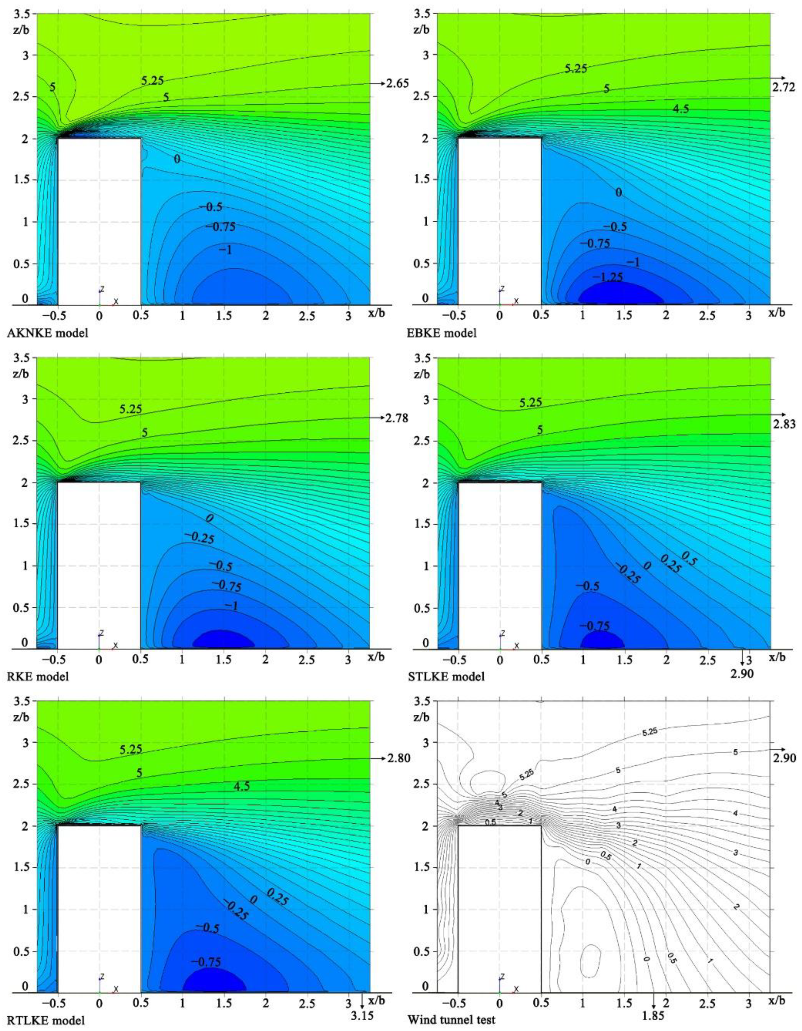
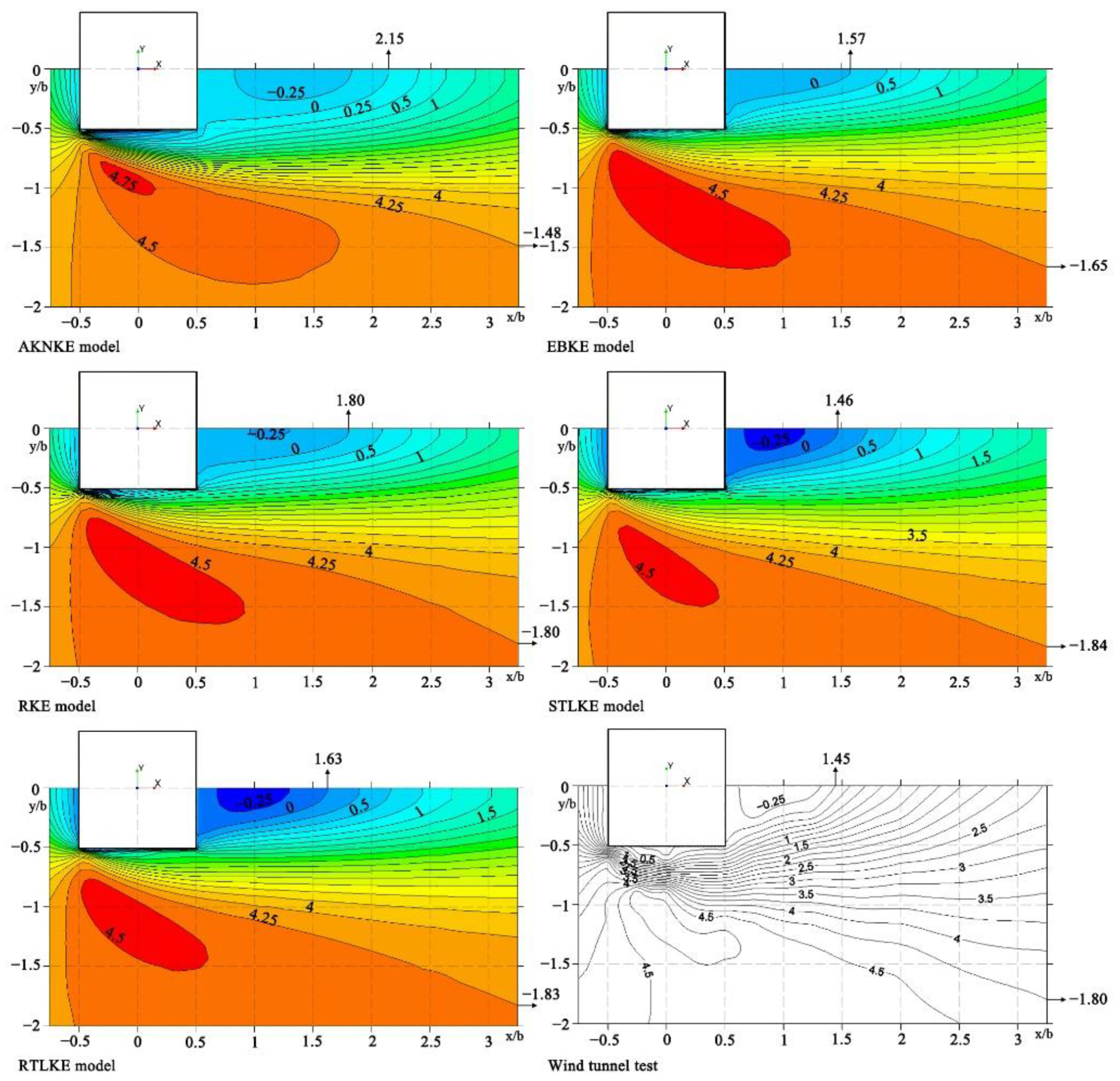
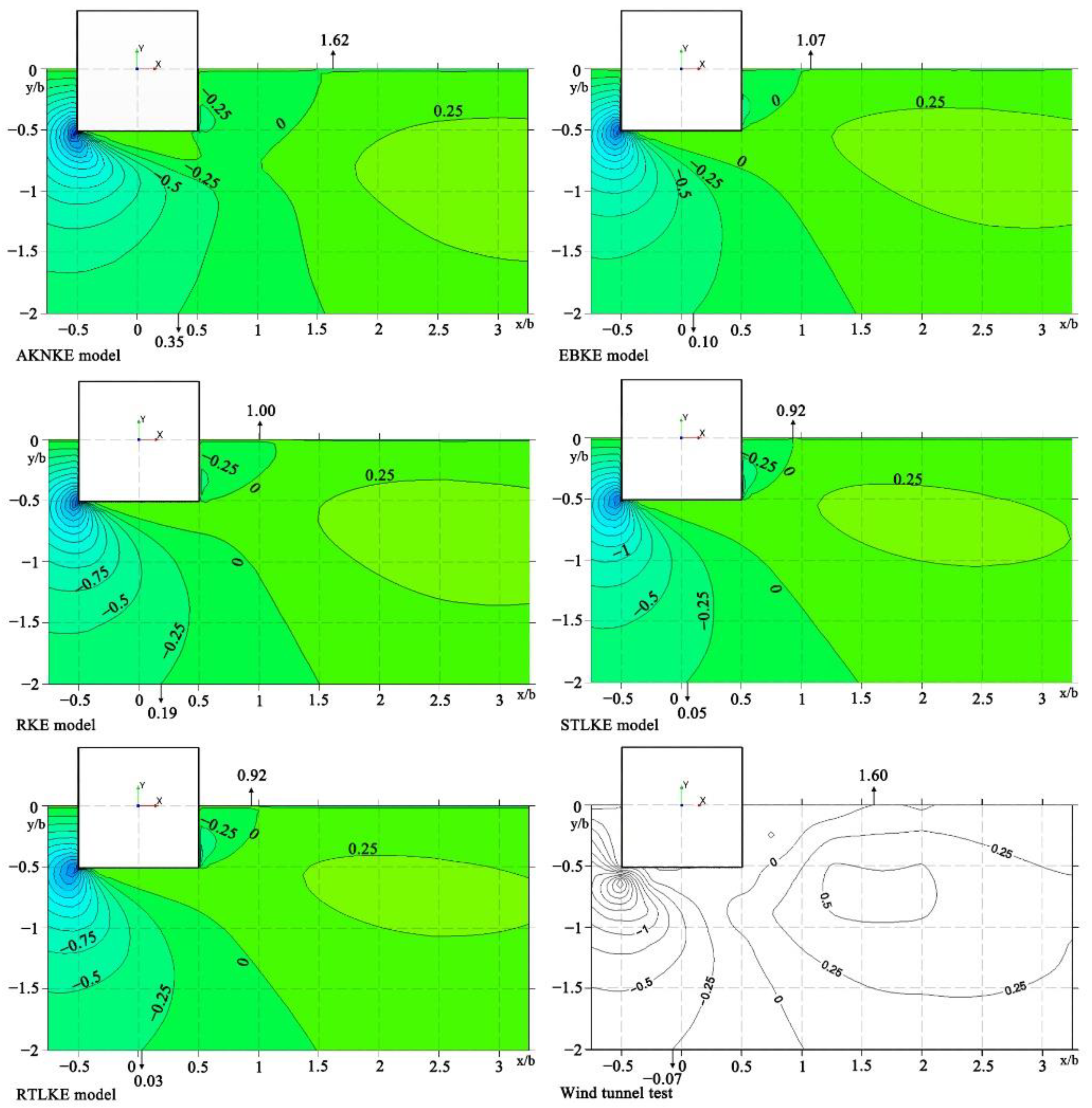
3.2.1. Comparison of Wind Speeds on the Vertical Plane at Y = 0

Figure 9 shows the contour plots of the X-velocity (U) at y = 0.

Table 4. Location of contour line at Y = 0 (U).

	AKNKE	EBKE	RKE	STLKE	RTLKE	Wind Tunnel Experiment
Location of contour line of 0 m/s in X-direction (low-wind-speed area)	>3.5	>3.5	>3.5	2.90	3.15	1.85
Location of contour line of 5 m/s in Z-direction (high-wind-speed area)	2.65	2.72	2.78	2.83	2.80	2.90

presents the locations of the contour line at y = 0 (U). For the contour line of the 0 m/s wind speed in the low-wind-speed area behind the building, the simulated x/b-values were all higher than the value of 1.85 from the wind tunnel experiment. Among them, the x/b-value for the STLKE model was 2.90, which was the closet to the value of 1.85 from the experiment, followed by the RTLKE model. The results of the other three models showed more significant differences compared with the experimental results.

For the contour line of the 5 m/s wind velocity in the high-wind-speed area above the building, all the turbulence models displayed a similar trend. The simulated z/b-values were all close to the value of 2.90 from the experiment. All the five models showed good performance in predicting flow separation above the building.

Figure 10 shows the contour plots of the Z-velocity (W) at Y = 0.

Table 5. Location of contour line at Y = 0 (W).

	AKNKE	EBKE	RKE	STLKE	RTLKE	Wind Tunnel Experiment
Location of the contour line of −0.25 m/s in Z-direction (low-wind-speed area)	0.45	0.45	0.45	0.75	0.65	1.05
Location of the contour line of 0.5 m/s in Z-direction (high-wind-speed area)	2.80	2.70	2.75	2.75	2.75	2.70

presents the locations of the contour line at y = 0 (W). For the contour line of the –0.25 m/s wind speed in the low-wind-speed area behind the building, the simulated z/b-values were all lower than the value of 1.05 from the wind tunnel experiment. Among them, the z/b-value for the STLKE model was 0.75, which was the closest to the value of 1.05 from the experiment, followed by the RTLKE model. Moreover, the difference between the results from the other three models and of the experiment were rather significant.

For the contour line of the 0.5 m/s wind speed in the high-wind-speed area above the building, the results from the five turbulence models demonstrated subtle differences compared with the wind tunnel experiment results, and the five simulated z/b-values were all close to the value of 2.70 from the experiment.

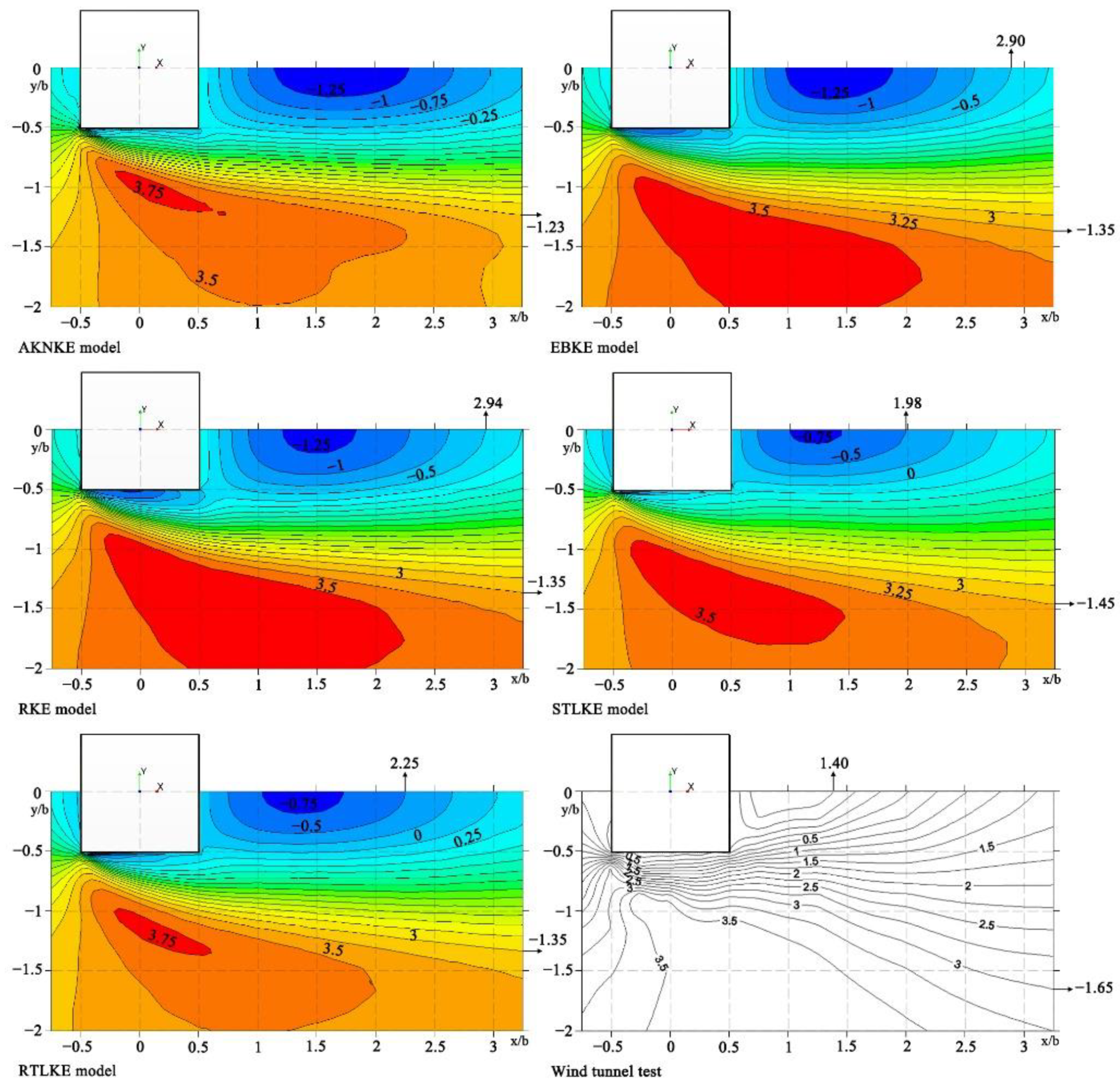
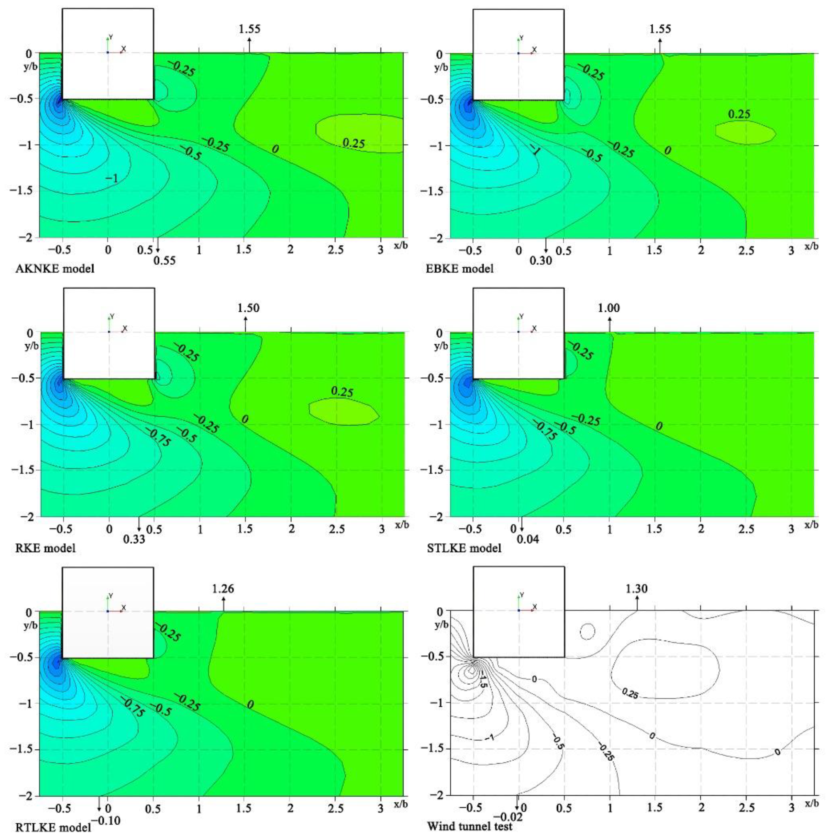
3.2.2. Comparison of Wind Speeds on the Horizontal Plane

Figure 11 shows the contour plots of the X-velocity (U) at z/b = 0.125.

Table 6. Location of contour line at z/b = 0.125 (U).

	AKNKE	EBKE	RKE	STLKE	RTLKE	Wind Tunnel Experiment
Location of the contour line of −0.5 m/s in X-direction (low-wind-speed area)	>3.5	2.90	2.94	1.98	2.25	1.40
Location of the contour line of 3 m/s in Y-direction (high-wind-speed area)	−1.23	−1.35	−1.35	−1.45	−1.35	−1.65

presents the locations of the contour line z/b = 0.125 (U). For the contour line of the −0.5 m/s wind speed in the low-wind-speed area behind the building, the simulated x/b-values were all higher than the value of 1.40 from the wind tunnel experiment. Among them, the x/b-value for the STLKE model was 1.98, which was the closest to the value of 1.40 from the experiment, followed by that of the RTLKE model. The results of the other three models were quite different from the experimental results.

For the contour line of the 3 m/s wind speed in the high-wind-speed area on the side of the building, the five simulated z/b-values were all higher than the value of −1.65 from the experiment. Among them, the z/b-value for the STLKE model was −1.45, which was the closest to the value of −1.65 from the experiment, followed by the results of the EBKE model, the RKE model, and the RTLKE model.

Figure 12 shows the contour plots of the Y-velocity (V) at z/b = 0.125.

Table 7. Location of contour line at z/b = 0.125 (V).

	AKNKE	EBKE	RKE	STLKE	RTLKE	Wind Tunnel Experiment
Location of the contour line of 0 m/s in X-direction (low-wind-speed area)	1.55	1.55	1.50	1.00	1.26	1.30
Location of the contour line of −0.5 m/s in X-direction (high-wind-speed area)	0.55	0.30	0.33	0.04	−0.10	−0.02

presents the locations of the contour line at z/b = 0.125 (V). For the contour line of the 0 m/s wind speed in the low-wind-speed area behind the building, the x/b-value for the STLKE model was 1.00 lower than the values for the other four models and lower than that from the experiment; the x/b-value for the RTLKE model was 1.26, which was the closest to the value of 1.30 from the experiment.

For the contour line of the −0.5 m/s wind speed in the high-wind-speed area on the side of the building, the x/b-value for the STLKE model was 0.04, which was the closest to the value of −0.02 from the experiment, followed by the results of the RTLKE model.

Figure 13 shows contour plots of the X-velocity (U) at z/b = 1.25.

Table 8. Location of contour line at z/b = 1.25 (U).

	AKNKE	EBKE	RKE	STLKE	RTLKE	Wind Tunnel Experiment
Location of the contour line of 0 m/s in X-direction (low-wind-speed area)	2.15	1.57	1.80	1.46	1.63	1.45
Location of the contour line of 4.25 m/s in Y-direction (high-wind-speed area)	−1.48	−1.65	−1.80	−1.84	−1.83	−1.80

presents the locations of the contour line at z/b = 1.25 (U). For the contour line of the 0 m/s wind speed in the low-wind-speed area behind the building, the x/b-value for the STLKE model was 1.46, which was the closest to the value of 1.45 from the experiment, followed by the EBKE model, the RTLKE model, and the RKE model. The x/b-value for the AKNKE model was 2.15, which was much higher than the value from the experiment.

For the contour line of the 4.25 m/s wind speed in the high-wind-speed area on the side of the building, the z/b-values for the RKE model, the STLRE model, and the RTLKE model were −1.80, −1.84, and −1.83, respectively, which were very close to the value of −1.80 from the experiment. The z/b-value for the AKNKE model was −1.48, much higher than the value from the experiment.

Figure 14 shows the contour plots of the Y-velocity (V) at z/b = 1.25.

Table 9. Location of contour line at z/b = 1.25 (V).

	AKNKE	EBKE	RKE	STLKE	RTLKE	Wind Tunnel Experiment
Location of the contour line of 0 m/s in X-direction (low-wind-speed area)	1.62	1.07	1.00	0.92	0.92	1.60
Location of the contour line of −0.25 m/s in X-direction (high-wind-speed area)	0.35	0.10	0.19	0.15	0.03	−0.07

presents the locations of the contour line at z/b = 1.25 (V). For the contour line of the 0 m/s wind speed in the low-wind-speed area behind the building, the x/b-value for the AKNKE model was 1.62, which was the closet to the value of 1.60 from the experiment. The other four simulated x/b-values were all much lower than the value from the experiment.

For the contour line of the −0.25 m/s wind speed in the high-wind-speed area on the side of the building, the x/b-value for the AKNKE model was 0.35, which was much higher than the value for the other four models and the experiment. The x/b-values for the other four models were all close to the value of −0.07 from the experiment. Among them, the x/b-value for the RTLKE model was 0.03, which was the closest to the value from the experiment.

Based on the cross-comparison of the wind speeds on the vertical and horizontal planes (

Table 10. Comparison of wind speeds in the low wind-speed area.

Location	Recommended Models	Not-Recommended Models (Much Different from the Experiment)
X-velocity (Y = 0)	STLKE, RTLKE	RKE, EBKE, AKNKE
Z-velocity (Y = 0)	STLKE, RTLKE	RKE, EBKE, AKNKE
X-velocity at z/b = 0.125	STLKE, RTLKE	RKE, EBKE, AKNKE
Y-velocity at z/b = 0.125	RTLKE	STLKE, RKE, EBKE, AKNKE
X-velocity at z/b = 1.25;	STLKE, RKE, RTLKE, EBKE	AKNKE
Y-velocity at z/b = 1.25	AKNKE	RKE, STLKE, RTLKE, EBKE
Total	RTLKE

and

Table 11. Comparison of wind speeds in the high wind-speed area.

Location	Recommended Models	Not-Recommended Models (Much Different from the Experiment)
X-velocity (Y = 0)	All
Z-velocity (Y = 0)	All
X-velocity at z/b = 0.125	STLKE, EBKE, RKE, RTLKE,	AKNKE
Y-velocity at z/b = 0.125	STLKE, RTLKE	RKE, EBKE, AKNKE
X-velocity at z/b = 1.25;	STLKE, RTLKE, RKE, EBKE	AKNKE
Y-velocity at z/b = 1.25	STLKE, RTLKE, EBKE, RKE	AKNKE
Total	STLKE, RTLKE	EBKE, RKE, AKNKE

), it was found that the STLKE model and the RTLKE model performed better in the high-wind-speed areas than the others; the RTLKE model also performed well in the low-wind-speed areas.

3.3. Comparison of Turbulent Kinetic Energy

3.3.1. Comparison of Turbulent Kinetic Energy at Y = 0

Figure 15 shows the contour plots of the turbulent kinetic energy at Y = 0.

Table 12. Location of contour line at Y = 0 (turbulent kinetic energy).

	AKNKE	EBKE	RKE	STLKE	RTLKE	Wind Tunnel Experiment
Location of the contour line of 0.5 in X-direction (low-wind-speed area)	0.90	2.05	>3.5	0.65	1.60	0.77
Location of the contour line of 1 in Z-direction (high-wind-speed area)	_	_	_	2.25	_	2.30

presents the locations of the contour line at Y = 0. Judging from the 0.5 contour line in the low-wind-speed area, the x/b-value for the STLKE model was 0.65, which was the closest to the value of 0.77 from the experiment, followed by the results from the AKNKE model and the RTLKE model. The x/b-value for the RKE model was higher than 3.5, which had large deviations in comparison with the experimental values.

By comparing the 1.0 contour lines of the simulation results and the wind tunnel experiment results in the high-wind-speed area, the z/b-value for the STLKE model was 2.25, which was quite close to the value of 2.30 from the experiment, while the other four models had large gaps with respect to the experimental results.

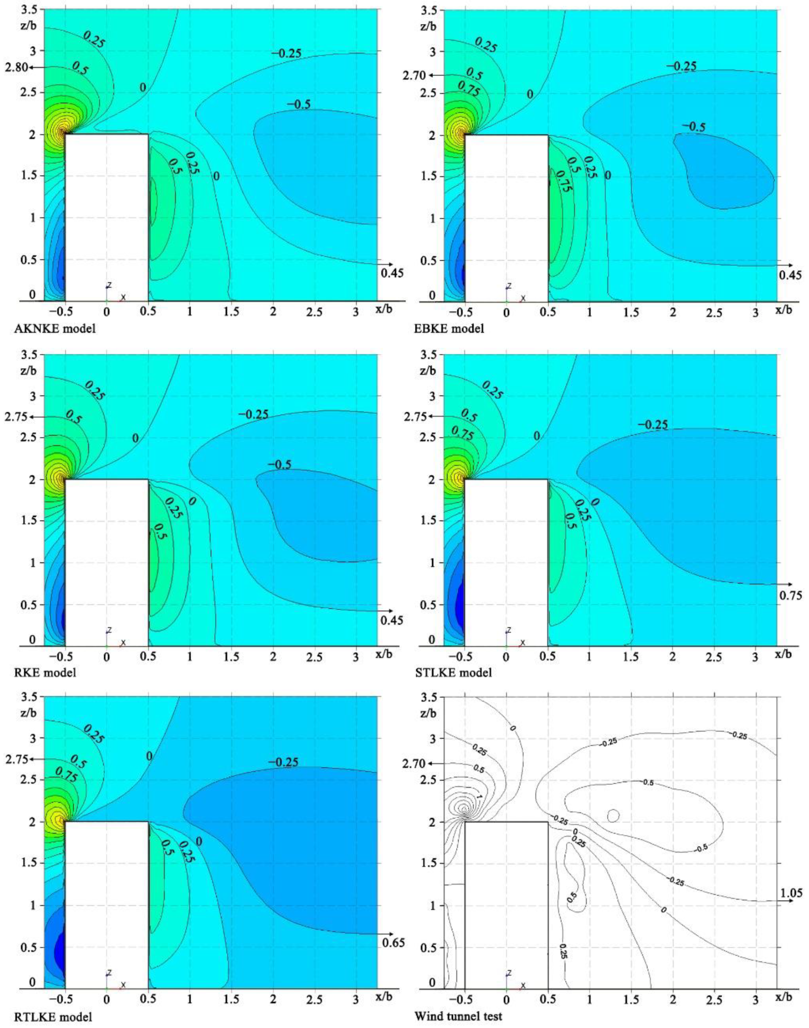
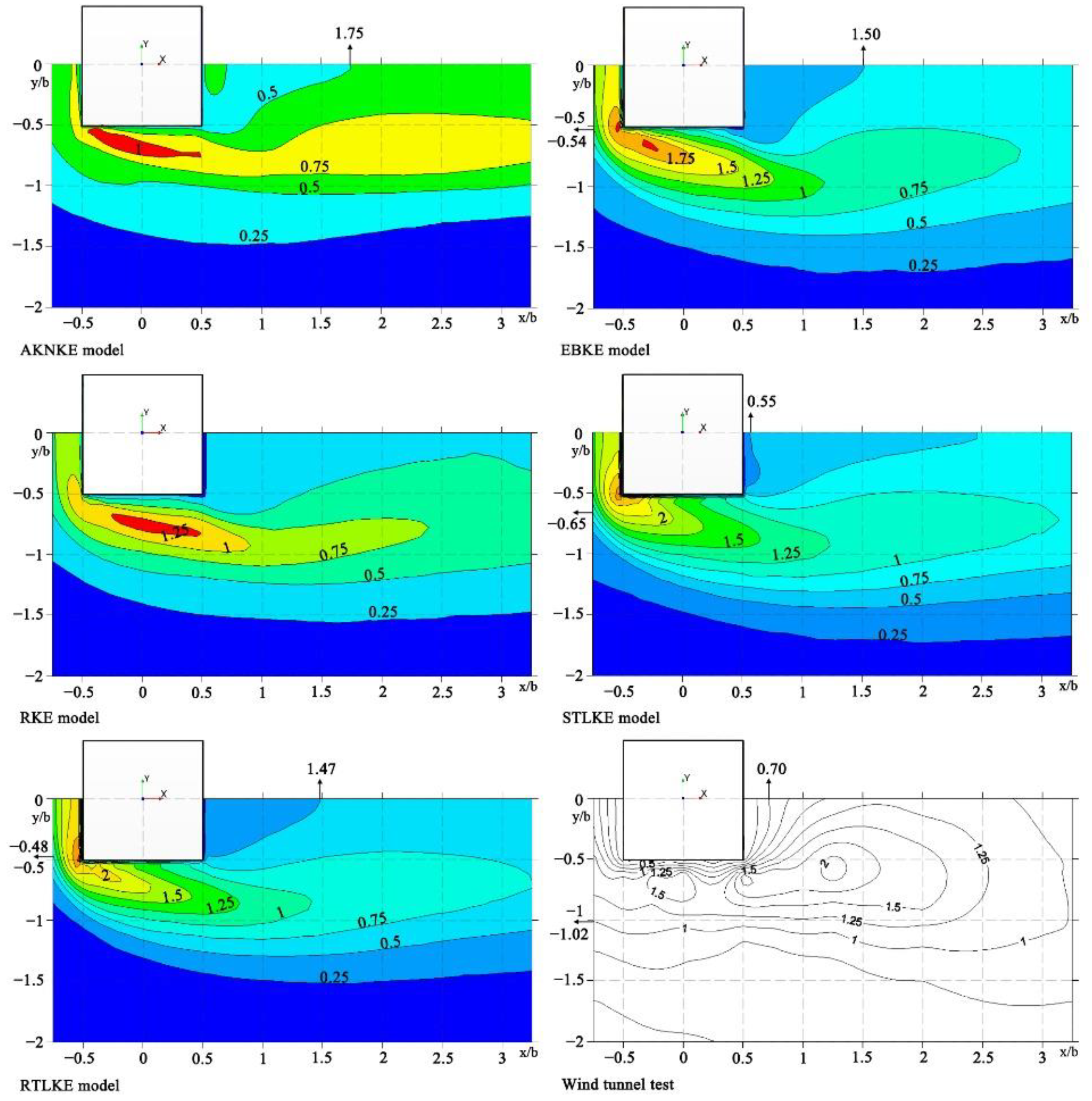
3.3.2. Comparison of Turbulent Kinetic Energy at z/b = 0.125

Figure 16 shows the contour plots of the turbulent kinetic energy at z/b = 0.125.

Table 13. Location of contour line at z/b = 0.125 (turbulent kinetic energy).

	AKNKE	EBKE	RKE	STLKE	RTLKE	Wind Tunnel Experiment
Location of the contour line of 0.5 in X-direction (low-wind-speed area)	1.75	1.50	-	0.55	1.47	0.70
Location of the contour line of 1 in Y-direction (high-wind-speed area)	-	−0.54	-	−0.65	−0.48	−1.02

presents the locations of the contour line at z/b = 0.125. From the 0.5 contour line in the low-wind-speed area, the x/b-value for the STLKE model was 0.55, which was the closest to the value of 0.70 from the experiment, followed by the values for the RTLKE model and the EBKE model, while the x/b-value for the AKNKE model was 1.75, which was much higher than the value from the experiment.

Based on the comparison of the 1 contour line in the high-wind-speed area between the simulation results and the wind tunnel experiment results, the z/b-value for the STLKE model was −0.65, which was the closest to the value of −1.02 from the experiment, followed by the results of the EBKE model and the RTLKE model, while the other two models had large gaps with respect to the experimental results.

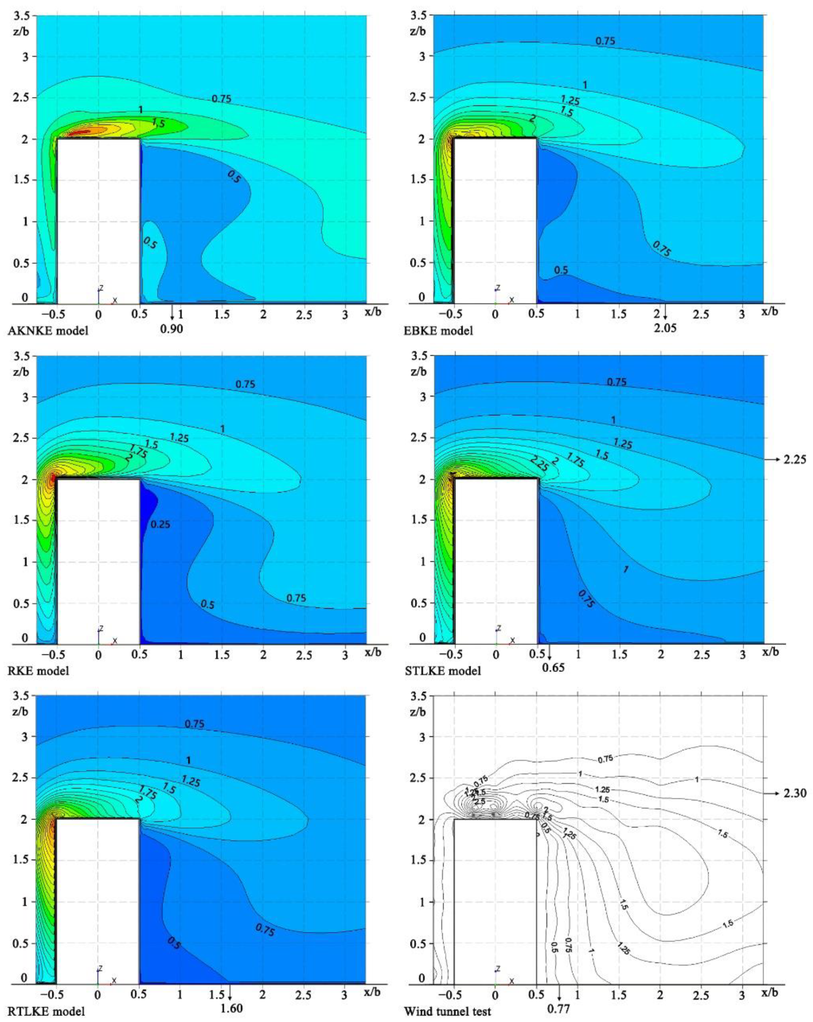
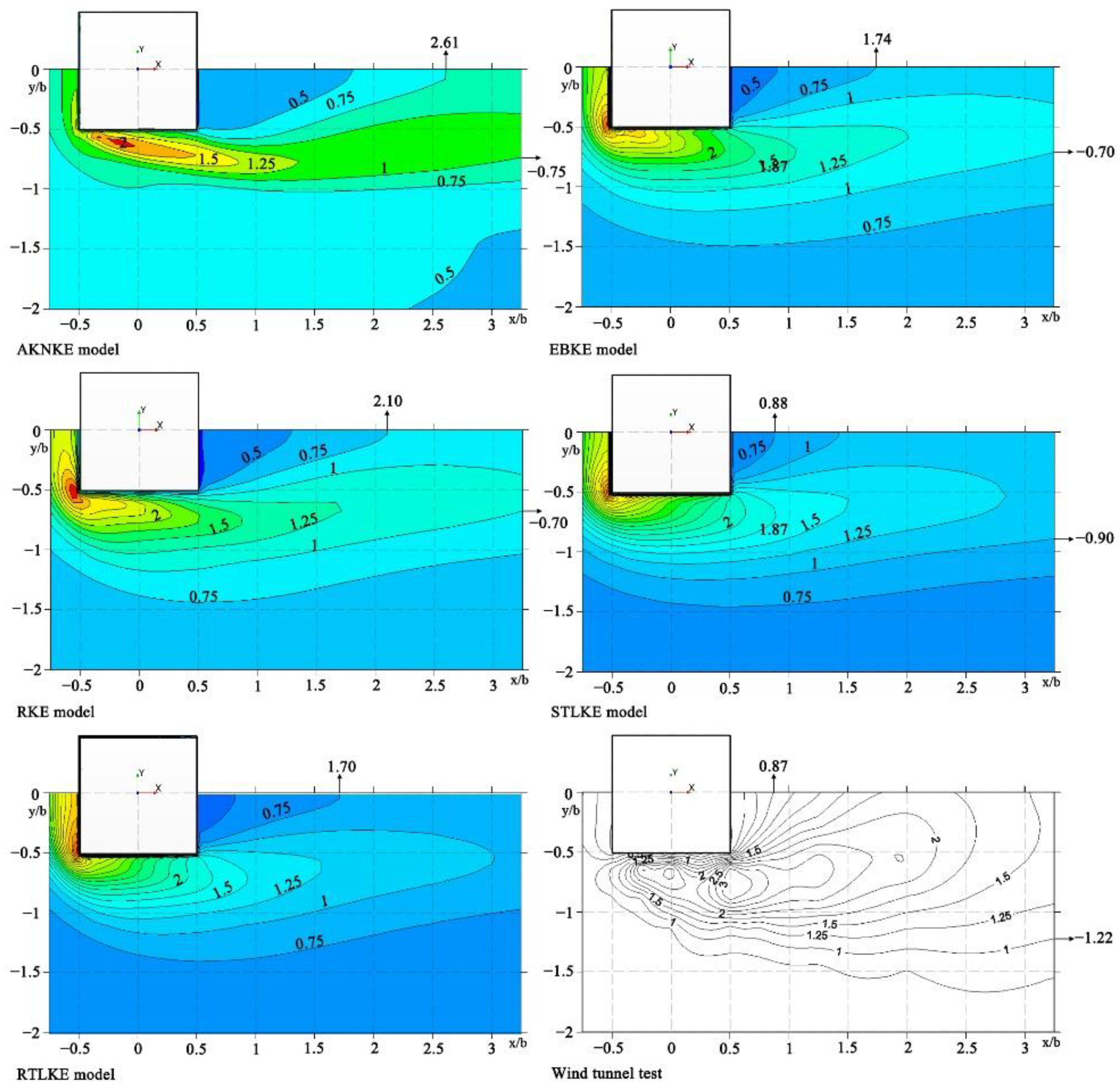
3.3.3. Comparison of Turbulent Kinetic Energy at z/b = 1.25

Figure 17 shows the contour plots of the turbulent kinetic energy at z/b = 1.25.

Table 14. Location of contour line at z/b = 1.25 (turbulent kinetic energy).

	AKNKE	EBKE	RKE	STLKE	RTLKE	Wind Tunnel Experiment
Location of the contour line of 0.75 in X-direction (low-wind-speed area)	2.61	1.74	2.10	0.88	1.70	0.87
Location of the contour line of 1 in Y-direction (high-wind-speed area)	−0.75	−0.70	−0.70	−0.90	-	−1.22

presents the locations of the contour line at z/b = 1.25. Judging from the 0.75 contour line in the low-wind-speed area, the x/b-value for the STLKE model was 0.88, which was quite close to the value of 0.87 from the experiment, followed by the results of the EBKE model and RTLKE model, while the values for the AKNKE model and the RKE model were quite different from those from the experiment.

Based on the comparison of the 1 contour line in the high-wind-speed area between the simulation results and the wind tunnel experiment results, the z/b-value for the STLKE model was −0.90, which was the closest to the value of −1.22 from the experiment, followed by the values for the AKNKE model, the EBKE model, and the RKE model, while the value for the RTLKE model was quite different from that from the experiment.

Based on the comparison of the turbulent kinetic energies on the vertical and horizontal planes (

Table 15. Comparison of turbulent kinetic energy in low wind-speed area.

Location	Recommended Models	Not-Recommended Models (Much Different from the Experiment)
Y = 0	STLKE, AKNKE, RTLKE	RKE, EBKE,
z/b = 0.125	STLKE, AKNKE, RTLKE	EBKE, RKE
z/b = 1.25	STLKE, RTLKE, EBKE	RKE, AKNKE
Total	STLKE, RTLKE	RKE, EBKE, AKNKE

and

Table 16. Comparison of turbulent kinetic energy in high wind-speed area.

Location	Recommended Models	Not-Recommended Models (Much Different from the Experiment)
Y = 0	STLKE	RTLKE, RKE, AKNKE, EBKE
z/b = 0.125	STLKE, EBKE, RTLKE	RKE, AKNKE
z/b = 1.25	STLKE, EBKE, RKE	RTLKE, AKNKE
	STLKE	RTLKE, RKE, AKNKE, EBKE

), the RTLKE model and the STLKE model performed better in the low-wind-speed area. In the high-wind-speed area, the STLKE model performed better than the other models.

4. Discussion

This research study shed light on the accuracy of CFD simulations. Previous research showed that the SKE model had some shortcomings in reproducing the low-speed-wind regions behind buildings, but modified k-ε models could improve these. In this study, various modified SKE models and RKE models (applied with the wall function, the damping function, etc.) were used to compare their efficiency, and the results were validated by comparing them to wind tunnel experiment results. It was found from this research study that: (a) There was a difference in wind speed between the experiment results and CFD predictions in the contour plots of the Y-velocity (V) at z/b = 0.125 (Figure 10). (b) There was also a difference in the turbulent kinetic energy between the experiment results and CFD predictions in the contour plots of the turbulent kinetic energy at z/b = 1.25. The study showed that using polyhedral meshes, the modified k-ε models could improve the accuracy of the simulations but could still not perfectly match the wind tunnel experiment results. The approach to optimize the closure coefficients of the RANS turbulence model or the method of coupling multiple models could improve the accuracy of CFD simulations, but they are difficult to be applied in engineering design because this approach requires engineers to master more professional knowledge of fluid dynamics. It is hoped that the existing models can be further modified based on these research findings and finally lead to a more accurate and more convenient toolkit for engineers.

Having said the above, the modified k-ε models are still widely used for design and analysis purposes in many engineering applications due to their low computational cost and data storage requirement. It was found from this study that:

(a)

In the low-wind-speed area, the STLKE model and the RTLKE model could predict turbulence kinetic energy in a more accurate way. The RTLKE model also performed well in predicting the wind speed on the vertical and horizontal planes. The RTLKE model could be used for simulations in research studies of low wind-speed areas to predict the size of the static-wind areas around high-rise buildings, the diffusion time of pollutants around buildings, etc.

(b)

In the high-wind-speed area, the STLKE model and the RTLKE model could accurately predict wind speed. Between them, the STLKE model performed better in simulating the turbulence kinetic energy. Therefore, the STLKE model is recommended to be used for simulations in research studies of high wind-speed areas (e.g., windward side) of high-rise buildings to predict the damage of high wind speed to the area around buildings during a typhoon, the maximum wind-speed area around high-rise buildings, etc.

Wind speed is considered important in current high-rise building designs. However, there is a lack of relevant guidelines or tools that could help designers predict outdoor wind environment. It is, therefore, hoped that findings from this research study supplement some existing building design guidance.

5. Conclusions

This paper simulated the wind flow around a high-rise building using different k-ε turbulence models with a polyhedral mesh system. The accuracy of the simulation results was evaluated against the AIJ wind tunnel experiment results. It was concluded that:

(1)

Under polyhedral mesh conditions, the modified k-e models applied with the wall function and the damping function improved the accuracy of the simulations but could still not perfectly match the wind tunnel experiment results. The correction of the models (e.g., optimizing the closure coefficients of the RANS turbulence model) needs to be further studied in order to significantly improve the accuracy of CFD simulations.

(2)

In the low-wind-speed area, the simulation results of the RTLKE model were the closest to the experimental results of the wind tunnels. In the high-wind-speed area, the simulation results of the STLKE model were the closest to the experimental results of the wind tunnels. So, these two models are recommended to be used for the simulation of wind around high-rise buildings under different circumstances.

(3)

In practice, it is recommended to use the STLKE model to explore high-wind-speed areas around high-rise buildings (e.g., the high-wind-speed areas around buildings during a typhoon, the maximum wind speed area around high-rise buildings, etc.). It is recommended to use the RTLKE model to explore low-wind-speed areas around high-rise buildings (e.g., the size of the static-wind area around high-rise buildings, the diffusion time of pollutants around buildings, etc.).

References

1. Blocken, B.; Carmeliet, J. Pedestrian Wind Environment around Buildings: Literature Review and Practical Examples. J. Therm. Envel. Build. Sci. 2004, 28, 107–159. [Google Scholar] [CrossRef]
2. Mittal, H.; Sharma, A.; Gairola, A. A review on the study of urban wind at the pedestrian level around buildings. J. Build. Eng. 2018, 18, 154–163. [Google Scholar] [CrossRef]
3. Uematsu, Y.; Yamada, M.; Higashiyama, H.; Orimo, T. Effects of the corner shape of high-rise buildings on the pedestrian-level wind environment with consideration for mean and fluctuating wind speeds. J. Wind Eng. Ind. Aerodyn. 1992, 44, 2289–2300. [Google Scholar] [CrossRef]
4. Liu, H.; Jiang, Y.; Liang, B.; Zhu, F.; Zhang, B.; Sang, J. Studies on wind environment around high buildings in urban areas. Sci. China Ser. D Earth Sci. 2005, 48, 102–115. [Google Scholar] [CrossRef]
5. Tsang, C.W.; Kwok, K.C.S.; Hitchcock, P.A. Wind tunnel study of pedestrian level wind environment around tall buildings: Effects of building dimensions, separation and podium. Build. Environ. 2012, 49, 167–181. [Google Scholar] [CrossRef]
6. Cheung, J.O.P.; Liu, C.-H. CFD Simulations of Natural Ventilation Behaviour in High-Rise Buildings in Regular and Staggered Arrangements at Various Spacing. Energy Build. 2011, 43, 1149–1158. [Google Scholar] [CrossRef]
7. Fang, P.; Zheng, D.; Gu, M.; Cheng, H.; Zhu, B. Numerical investigation of the wind environment around tall buildings in a central business district. Front. Earth Sci. 2019, 13, 848–858. [Google Scholar] [CrossRef]
8. Tominaga, Y.; Shirzadi, M. Wind tunnel measurement of three-dimensional turbulent flow structures around a building group: Impact of high-rise buildings on pedestrian wind environment. Build. Environ. 2021, 206, 108389. [Google Scholar] [CrossRef]
9. Yim, S.H.L.; Fung, J.; Lau, A.; Kot, S.C. Air ventilation impacts of the “wall effect” resulting from the alignment of high-rise buildings. Atmos. Environ. 2009, 43, 4982–4994. [Google Scholar] [CrossRef]
10. Aristodemou, E.; Boganegra, L.; Mottet, L.; Pavlidis, D.; Constantinou, A.; Pain, C.; Robins, A.; Apsimon, H. How tall buildings affect turbulent air flows and dispersion of pollution within a neighbourhood. Environ. Pollut. 2017, 233, 782–796. [Google Scholar] [CrossRef]
11. Liu, X.P.; Niu, J.; Kwok, K.C.S.; Wang, J.H.; Li, B.Z. Investigation of indoor air pollutant dispersion and cross-contamination around a typical high-rise residential building: Wind tunnel tests. Build. Environ. 2010, 45, 1769–1778. [Google Scholar] [CrossRef]
12. Qiao, W.; Wang, Y.; Zhang, J.; Tian, W.; Tian, Y.; Yang, Q. An innovative coupled model in view of wavelet transform for predicting short-term PM10 concentration. J. Environ. Manag. 2021, 289, 112438. [Google Scholar] [CrossRef] [PubMed]
13. Qiao, W.; Li, Z.; Liu, W.; Liu, E. Fastest-growing source prediction of US electricity production based on a novel hybrid model using wavelet transform. Int. J. Energy Res. 2022, 46, 1766–1788. [Google Scholar] [CrossRef]
14. Paterson, D.; Apelt, C. Computation of wind flows over three-dimensional buildings. J. Wind Eng. Ind. Aerodyn. 1986, 24, 193–213. [Google Scholar] [CrossRef]
15. Shirasawa, T.; Endo, Y.; Yoshie, R.; Mochida, A.; Tanaka, H. Comparison of les and durbin type k-ε model for gas diffusion in weak wind region behind a building. J. Environ. Eng. 2008, 73, 615–622. [Google Scholar] [CrossRef] [Green Version]
16. Tominaga, Y. Flow around a high-rise building using steady and unsteady RANS CFD: Effect of large-scale fluctuations on the velocity statistics. J. Wind Eng. Ind. Aerodyn. 2015, 142, 93–103. [Google Scholar] [CrossRef]
17. Revuz, J.; Hargreaves, D.; Owen, J. On the domain size for the steady-state CFD modelling of a tall building. Wind Struct. 2012, 15, 313–329. [Google Scholar] [CrossRef]
18. Kim, J.-C.; Lee, K.-S. Effect of Grid Size on Building Wind According to a Computation Fluid Dynamics Simulation. Asia Pac. J. Atmos. Sci. 2011, 47, 193–198. [Google Scholar] [CrossRef]
19. Murakami, S.; Mochida, A. Three-Dimensional Numerical Simulation of Turbulent Flow Around Buildings using the k-e Turbulence Model. Build. Environ. 1989, 24, 51–64. [Google Scholar] [CrossRef]
20. Tan, Y.; Li, C. Simulation of Wind Effects Embracing a Complex Shape Super High-Rise Steel TV Tower Using CFD. Adv. Mater. Res. 2011, 201–203, 2807–2813. [Google Scholar] [CrossRef]
21. Behrouzi, F.; Sidik, N.A.C.; Malik, A.M.A.; Nakisa, M. Prediction of Wind Flow around High-Rise Buildings Using RANS Models. Appl. Mech. Mater. 2014, 554, 724–729. [Google Scholar] [CrossRef]
22. Yoshie, R.; Mochida, A.; Tominaga, Y.; Kataoka, H.; Harimoto, K.; Nozu, T.; Shirasawa, T. Cooperative project for CFD prediction of pedestrian wind environment in the Architectural Institute of Japan. J. Wind Eng. Ind. Aerodyn. 2007, 95, 1551–1578. [Google Scholar] [CrossRef]
23. Tominaga, Y.; Stathopoulos, T. Numerical simulation of dispersion around an isolated cubic building: Model evaluation of RANS and LES. Build. Environ. 2010, 45, 2231–2239. [Google Scholar] [CrossRef] [Green Version]
24. Vardoulakis, S.; Dimitrova, R.; Richards, K.; Hamlyn, D.; Camilleri, G.; Weeks, M.; Sini, J.-F.; Britter, R.; Borrego, C.; Schatzmann, M.; et al. Numerical Model Inter-comparison for Wind Flow and Turbulence Around Single-Block Buildings. Environ. Model. Assess. 2011, 16, 169–181. [Google Scholar] [CrossRef]
25. Gousseau, P.; Blocken, B.; van Heijst, G.J.F. CFD simulation of pollutant dispersion around isolated buildings: On the role of convective and turbulent mass fluxes in the prediction accuracy. J. Hazard. Mater. 2011, 194, 422–434. [Google Scholar] [CrossRef]
26. Zhang, Z.P.; Zhang, W.; Chen, G.P. Numerical Simulation of Flow around High-Rise Buildings Based on Reynolds Stress Model. Appl. Mech. Mater. 2014, 580–583, 3057–3061. [Google Scholar] [CrossRef]
27. Tominaga, Y.; Mochida, A.; Murakami, S.; Sawaki, S. Comparison of various revised k–ε models and LES applied to flow around a high-rise building model with 1:1:2 shape placed within the surface boundary layer. J. Wind Eng. Ind. Aerodyn. 2008, 96, 389–411. [Google Scholar] [CrossRef]
28. Thordal, M.S.; Bennetsen, J.C.; Koss, H.H.H. Review for practical application of CFD for the determination of wind load on high-rise buildings. J. Wind Eng. Ind. Aerodyn. 2019, 186, 155–168. [Google Scholar] [CrossRef]
29. Thordal, M.S.; Bennetsen, J.C.; Capra, S.; Koss, H.H.H. Towards a standard CFD setup for wind load assessment of high-rise buildings: Part 1—Benchmark of the CAARC building. J. Wind. Eng. Ind. Aerodyn. 2020, 205, 104283. [Google Scholar] [CrossRef]
30. Thordal, M.S.; Bennetsen, J.C.; Capra, S.; Kragh, A.K.; Koss, H.H.H. Towards a standard CFD setup for wind load assessment of high-rise buildings: Part 2—Blind test of chamfered and rounded corner high-rise buildings. J. Wind. Eng. Ind. Aerodyn. 2020, 205, 104282. [Google Scholar] [CrossRef]
31. Liu, J.; Niu, J. CFD simulation of the wind environment around an isolated high-rise building: An evaluation of SRANS, LES and DES models. Build. Environ. 2016, 96, 91–106. [Google Scholar] [CrossRef]
32. Shirzadi, M.; Mirzaei, P.A.; Naghashzadegan, M. Improvement of k-epsilon turbulence model for CFD simulation of atmospheric boundary layer around a high-rise building using stochastic optimization and Monte Carlo Sampling technique. J. Wind Eng. Ind. Aerodyn. 2017, 171, 366–379. [Google Scholar] [CrossRef]
33. Shirzadi, M.; Mirzaei, P.A.; Tominaga, Y. RANS model calibration using stochastic optimization for accuracy improvement of urban airflow CFD modeling. J. Build. Eng. 2020, 32, 101756. [Google Scholar] [CrossRef]
34. Du, Y.; Mak, C.M.; Ai, Z. Modelling of pedestrian level wind environment on a high-quality mesh: A case study for the HKPolyU campus. Environ. Modell. Softw. 2018, 103, 105–119. [Google Scholar] [CrossRef]
35. Nozu, T.; Tamura, T.; Takeshi, K.; Akira, K. Mesh-adaptive LES for wind load estimation of a high-rise building in a city. J. Wind Eng. Ind. Aerodyn. 2015, 144, 62–69. [Google Scholar] [CrossRef]
36. Blocken, B.; Carmeliet, J. Pedestrian wind conditions at outdoor platforms in a high-rise apartment building: Generic sub-configuration validation, wind comfort assessment and uncertainty issues. Wind Struct. 2008, 11, 51–70. [Google Scholar] [CrossRef] [Green Version]
37. Sosnowski, M.; Gnatowska, R.; Grabowska, K.; Krzywański, J.; Jamrozik, A. Numerical Analysis of Flow in Building Arrangement: Computational Domain Discretization. Appl. Sci. 2019, 9, 941. [Google Scholar] [CrossRef] [Green Version]
38. China Academy of Building Research. Assessment Standard for Green Building, GB/T 50378-2019; Ministry of Housing and Urban-rural Development of the People’s Republic of China: Beijing, China, 2019; pp. 30–31.
39. Meng, Y.; Hibi, K. Turbulent measurements of the flow field around a high-rise buildings. Wind Eng. JAWE 1998, 76, 55–64. [Google Scholar] [CrossRef]
40. Mochida, A.; Tominaga, Y.; Murakami, S.; Yoshie, R.; Ishihara, T.; Ooka, R. Comparison of various k-e models and DSM applied to flow around a high rise building report on AIJ cooperative project for CFD prediction of wind environment. Wind Struct. 2002, 5, 227–244. [Google Scholar] [CrossRef] [Green Version]
41. Franke, J.; Hellsten, A.; Schlünzen, K.; Carissimo, B. Best practice guideline for the CFD simulation of flows in the urban environment-a summary. In Proceedings of the 11th Conference on Harmonisation within Atmospheric Dispersion Modelling for Regulatory Purposes, Cambridge, UK, 2–5 July 2007. [Google Scholar]
42. Blocken, B. Computational Fluid Dynamics for urban physics: Importance, scales, possibilities, limitations and ten tips and tricks towards accurate and reliable simulations. Build. Environ. 2015, 91, 219–245. [Google Scholar] [CrossRef] [Green Version]
43. Tominaga, Y.; Mochida, A.; Yoshie, R.; Kataoka, H.; Nozu, T.; Yoshikawa, M.; Shirasawa, T. AIJ guidelines for practical applications of CFD to pedestrian wind environment around buildings. J. Wind Eng. Ind. Aerodyn. 2008, 96, 1749–1761. [Google Scholar] [CrossRef]
44. Jones, W.P.; Launder, B.E. The prediction of laminarization with a two-equation model of turbulence. Int. J. Heat Mass Transf. 1972, 15, 301–314. [Google Scholar] [CrossRef]
45. Wolfshtein, M. The velocity and temperature distribution in one-dimensional flow with turbulence augmentation and pressure gradient. Int. J. Heat Mass Transf. 1969, 12, 301–318. [Google Scholar] [CrossRef]
46. Lien, F.S.; Chen, W.L.; Leschziner, M. Low-Reynolds-Number Eddy-Viscosity Modelling Based on Non-Linear Stress-Strain/Vorticity Relations. In Engineering Turbulence Modelling and Experiments; Rodi, W., Bergeles, G., Eds.; Elsevier: Oxford, UK, 1996; Volume 3, pp. 91–100. [Google Scholar]
47. Shih, T.-H.; Liou, W.W.; Shabbir, A.; Yang, Z.; Zhu, J. A new k-ϵ eddy viscosity model for high reynolds number turbulent flows. Comput. Fluids 1995, 24, 227–238. [Google Scholar] [CrossRef]
48. Abe, K.; Kondoh, T.; Nagano, Y. A new turbulence model for predicting fluid flow and heat transfer in separating and reattaching flows—II. Thermal field calculations. Int. J. Heat Mass Transf. 1995, 38, 1467–1481. [Google Scholar] [CrossRef]
49. Durbin, P.A. A Reynolds stress model for near-wall turbulence. J. Fluid Mech. 1993, 249, 465–498. [Google Scholar] [CrossRef]
50. Lien, F.S.; Kalitzin, G.; Durbin, P.A. RANS modeling for compressible and transitional flows. In Proceedings of the Summer Program, Stanford, CA, USA; 1998; pp. 267–286. [Google Scholar]
51. Durbin, P.A. On the k-3 stagnation point anomaly. Int. J. Heat Fluid Flow 1996, 17, 89–90. [Google Scholar] [CrossRef]
52. Zhang, H.; Xiong, M.; Chen, B.; Wang, Y. Influence of Tropical Cyclones on Outdoor Wind Environment in High-Rise Residential Areas in Zhejiang Province, China. Sustainability 2022, 14, 3932. [Google Scholar] [CrossRef]
53. Qin, H.; Lin, P.; Lau, S.S.Y.; Song, D. Influence of site and tower types on urban natural ventilation performance in high-rise high-density urban environment. Build. Environ. 2020, 179, 106960. [Google Scholar] [CrossRef]
54. Adams, E.W.; Johnston, J.P. Effects of the separating shear layer on the reattachment flow structure part 2: Reattachment length and wall shear stress. Exp. Fluids 1988, 6, 493–499. [Google Scholar] [CrossRef]
55. Mochida, A.; Tominaga, Y.; Ishida, Y.; Ishihara, T.; Uehara, K.; Kataoka, H.; Kurabuchi, T.; Kobayashi, N.; Ooka, R.; Shirasawa, T.; et al. AIJ Benchmarks for Validation of CFD Simulations Applied to Pedestrian Wind Environment around Buildings; Architectural Institute of Japan: Tokyo, Japan, 2016. [Google Scholar]
Figure 1. Flowchart of this research work.
Applsci 12 07105 g001
Figure 2. High-rise building and computational domain.
Applsci 12 07105 g002
Figure 3. Wind speed and turbulent kinetic energy measurements.
Applsci 12 07105 g003
Figure 4. Location and size of blocks.
Applsci 12 07105 g004
Figure 5. Distribution of wind-speed test points: (a) distribution on the xz-plane (y = 0), (b) distribution on the xy-plane (z = 0.125b and z = 1.25b).
Applsci 12 07105 g005
Figure 6. Error values and calculation time.
Applsci 12 07105 g006
Figure 7. Section of mesh scheme for Case 2.
Applsci 12 07105 g007
Figure 8. Schematic diagram of XR and XF.
Applsci 12 07105 g008
Figure 9. Contour plots of X-velocity (U) at Y = 0.
Applsci 12 07105 g009
Figure 10. Contour plots of Z-velocity (W) at Y = 0.
Applsci 12 07105 g010
Figure 11. Contour plots of X-velocity (U) at z/b = 0.125.
Applsci 12 07105 g011
Figure 12. Contour plots of Y-velocity (V) at z/b = 0.125.
Applsci 12 07105 g012
Figure 13. Contour plots of X-velocity (U) at z/b = 1.25.
Applsci 12 07105 g013
Figure 14. Contour plots of Y-velocity (V) at z/b = 1.25.
Applsci 12 07105 g014
Figure 15. Contour plots of turbulent kinetic energy at Y = 0.
Applsci 12 07105 g015
Figure 16. Contour plots of turbulent kinetic energy at z/b = 0.125.
Applsci 12 07105 g016
Figure 17. Contour plots of turbulent kinetic energy at z/b = 1.25.
Applsci 12 07105 g017