Intra-Domain Transfer Learning for Fault Diagnosis with Small Samples

Abstract

The concept of deep transfer learning has spawned broad research into fault diagnosis with small samples. A considerable covariate shift between the source and target domains, however, could result in negative transfer and lower fault diagnosis task accuracy. To alleviate the adverse impacts of negative transfer, this research proposes an intra-domain transfer learning strategy that makes use of knowledge from a data-abundant source domain that is akin to the target domain. Concretely, a pre-trained model in the source domain is built via a vanilla transfer from an off-the-shelf inter-domain deep neural network. The model is then transferred to the target domain using shallow-layer freezing and finetuning with those small samples. In a case study involving rotating machinery, where we tested the proposed strategy, we saw improved performance in both training efficiency and prediction accuracy. To demystify the learned neural network, we propose a heat map visualization method using a channel-wise average over the final convolutional layer and up-sampling with interpolation. The findings revealed that the most active neurons coincide with the corresponding fault characteristics.

1. Introduction

Fault diagnosis is a crucial aspect of system safety and dependability [1], as it can pinpoint fault locations, identify fault types, and even gauge the severity of certain faults [2]. Existing approaches to fault diagnosis can generally be categorized as either model-based or data-driven [3]. The former approach necessitates a deep understanding of the subject matter since it builds a mathematical model of the subject of interest based on its first principles. The latter employs machine learning, statistics, signal processing, and other techniques to perform pattern recognition on monitoring data. Data-driven approaches are becoming more popular since they have a lower barrier to entry [4,5].

Data-driven approaches typically rely on a large amount of training samples to learn patterns that can be generalized to testing instances [6,7]. However, samples of faulty types are insufficient in many real-world applications, leading to an imbalanced classification problem [8]. Oversampling and down-sampling techniques may be used to create a more balanced dataset [9], but this introduces a bias, wherein more samples are selected from one class than another. Another workaround is data augmentation by learning the underlying generating mechanisms of scarce classes using generative models, such as a Variational Auto-Encoder (VAE) [10] or a Generative Adversarial Network (GAN) [11,12]. Though some success has been reported, it is a paradox to learn from data that are rare to synthesize more data.

Deep transfer learning has been adopted to address the issue of small samples in fault diagnosis, with the hope of reutilizing the knowledge learned from a source task in a target task [13]. Importantly, the number of samples required for training in the target task can be greatly reduced. In one study, an enhanced deep auto-encoder model was proposed to transfer the knowledge learned from a data-abundant source domain to a data-scarce target domain for the purpose of fault diagnosis [14]. Elsewhere, deep transfer learning was applied to transfer knowledge among various operating modes of rotating machinery, including rotational speed [15] and working load [16,17].

However, negative transfer may occur if source and target domains have significant differences; i.e., if domain-specific samples have large discrepancies in their probability distributions [18]. In other words, bringing source domain knowledge into the target task does not help, but rather hinders performance. The effect of negative transfer has been noted in several transfer-learning-enabled fault diagnosis applications [15,18,19], inspiring researchers to examine the causes of negative transfer. A review can be found in [20,21].

Although the factors contributing to negative transfer are multifaceted, the primary cause is rooted in a covariate shift between source and target domains [21,22]. Therefore, domain adaptation measures have been proposed to prevent negative transfer or mitigate its adverse impact, including source data filtering using an adversarial approach [22], new architectural design [23,24,25], the use of transitive transfer strategy [26], etc. Although many negative transfer countermeasures have been developed, transferring a pretrained model directly from a distant inter-domain to the target domain still poses problems [27,28]. More specifically, there is a knowledge gap on how to mitigate negative transfer in transfer learning with small samples in fault diagnosis tasks. This gap constitutes the major motivation of this study.

Inspired by the work in [26], where intermediate domains were implanted to bridge the gap between distant source and target domains, we propose an intra-domain learning strategy to explicitly utilize the knowledge of a distribution-alike source domain for the purpose of fault diagnosis with small samples. Concretely, we conduct a vanilla transfer from an off-the-shelf inter-domain deep learning model to a data-abundant source domain. The model is then transferred to the target task via shallow-layer freezing and finetuning. The intra-domain transfer learning strategy is the primary novelty of this research. We validate the proposed strategy in a case study with varying levels of small sample ratios and observe its efficacy over alternatives in terms of convergence speed and diagnostic accuracy. This study empirically proves the soundness and merit of transferring among distribution-alike domains in the field of fault diagnosis. We argue cautions against a direct transfer among inter-domains should be issued to reduce the risk of committing negative transfer.

To have an intuitive understanding of the learned model, we produce heat maps to visualize the learned high-level features of the input data. Unlike traditional Class Activation Mapping methods, our novel method uses a channel-wise average over the final convolutional layer and up-sampling with interpolation. Heat map visualization verifies the proposed strategy can extract fault-related characteristics.

The contributions of this research are twofold: (1) we propose an intra-domain transfer learning strategy and a fault diagnosis model for rotating equipment under the scenario of small samples; (2) we propose a novel heat map visualization method to demystify the transferred deep learning model.

The remaining sections are organized as follows. Section 2 explains the intra-domain transfer learning strategy and introduces a rotating equipment fault diagnosis model based on vibration data. Section 3 validates the proposed strategy and model in a case study of a gearbox dataset. Section 4 demonstrates the heat map method and provides a visual portrayal of the features extracted by the transferred deep learning model. Section 5 concludes the work.

2. Methodology

This section introduces the intra-domain transfer learning strategy and elucidates a fault diagnosis model using the proposed strategy.

2.1. Intra-Domain Transfer Learning Strategy

Transfer learning refers to the application of experiences gained in solving one task to a different but similar task. Experiences learned from the source domain are used as prior knowledge to solve target problems. Put formally, given a source domain $D_S$ and a target domain $D_T$, transfer learning reuses the information embedded in $D_S$ for better problem-solving in $D_T$. Through knowledge sharing, the requirements for supervisory instances in $D_T$ can be greatly reduced, thus making it possible to learn even when samples are small.

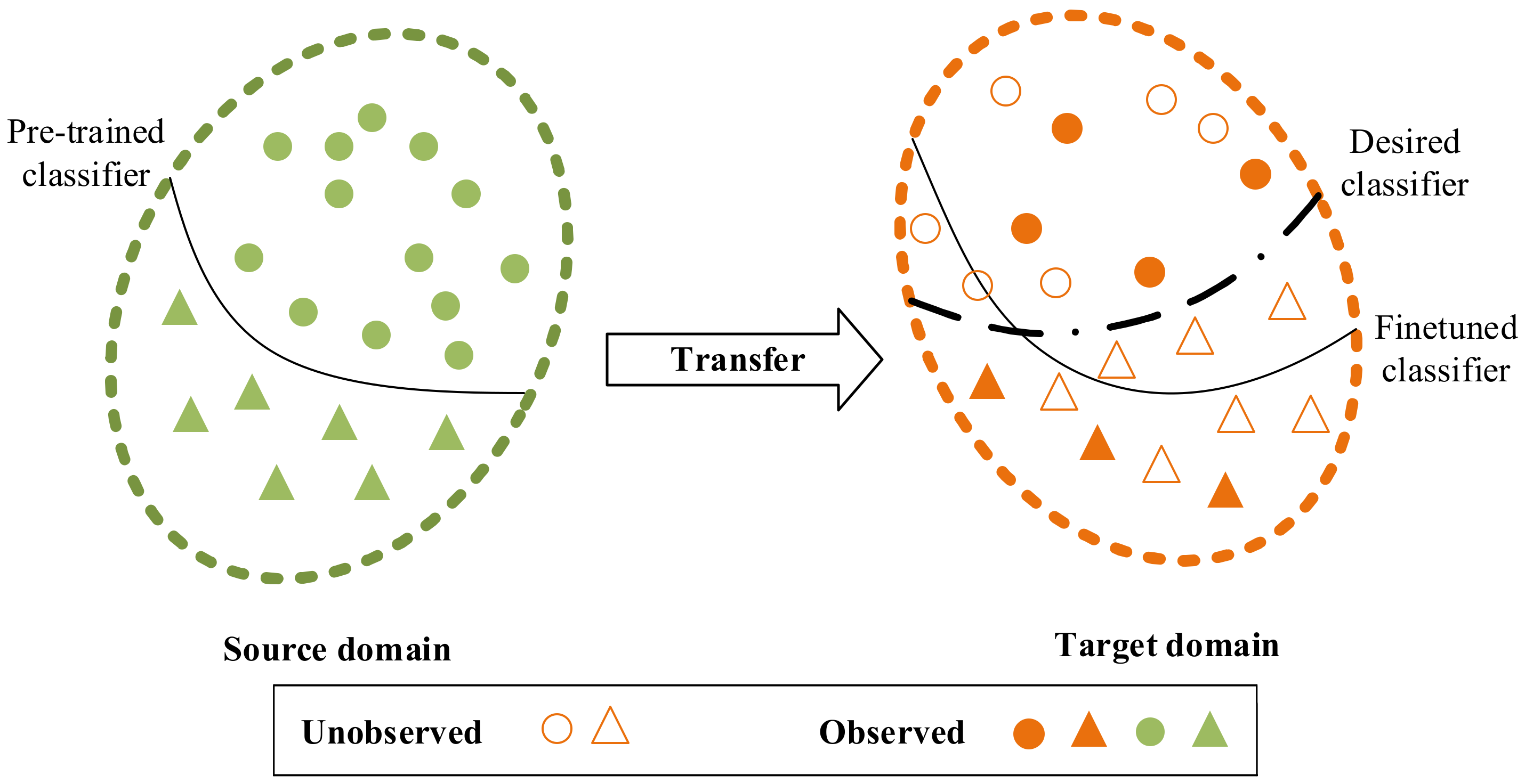
The above statement holds true in general when the source and target domains are closely related. However, if there is a significant covariate shift between $D_S$ and $D_T$, transfer learning might inversely hurt the target performance, i.e., negative transfer [22,26]; see Figure 1. In other words, inter-domain transfer may take the learning in the wrong direction in the target domain. To mitigate the impact of negative transfer, researchers have proposed many workarounds, including instance weighting [29], feature matching [30], and transitive transfer [31]. Inspired by the Distant Domain Transfer Learning (DDTL) approach in [26] where domain discrepancies are substantial, we propose an intra-domain transfer learning strategy.

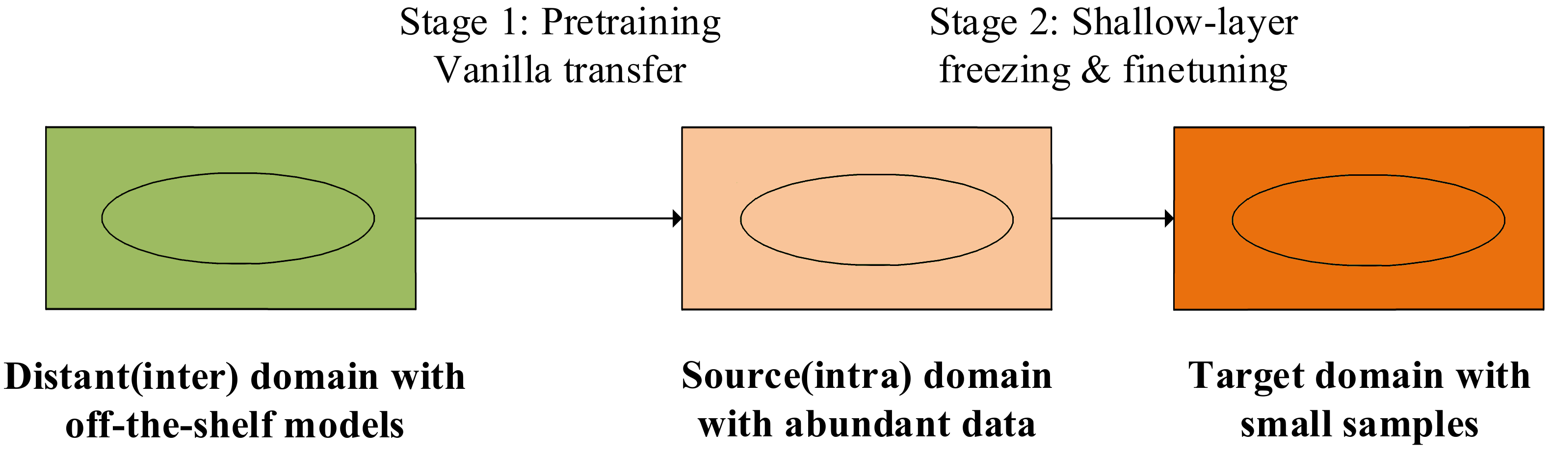
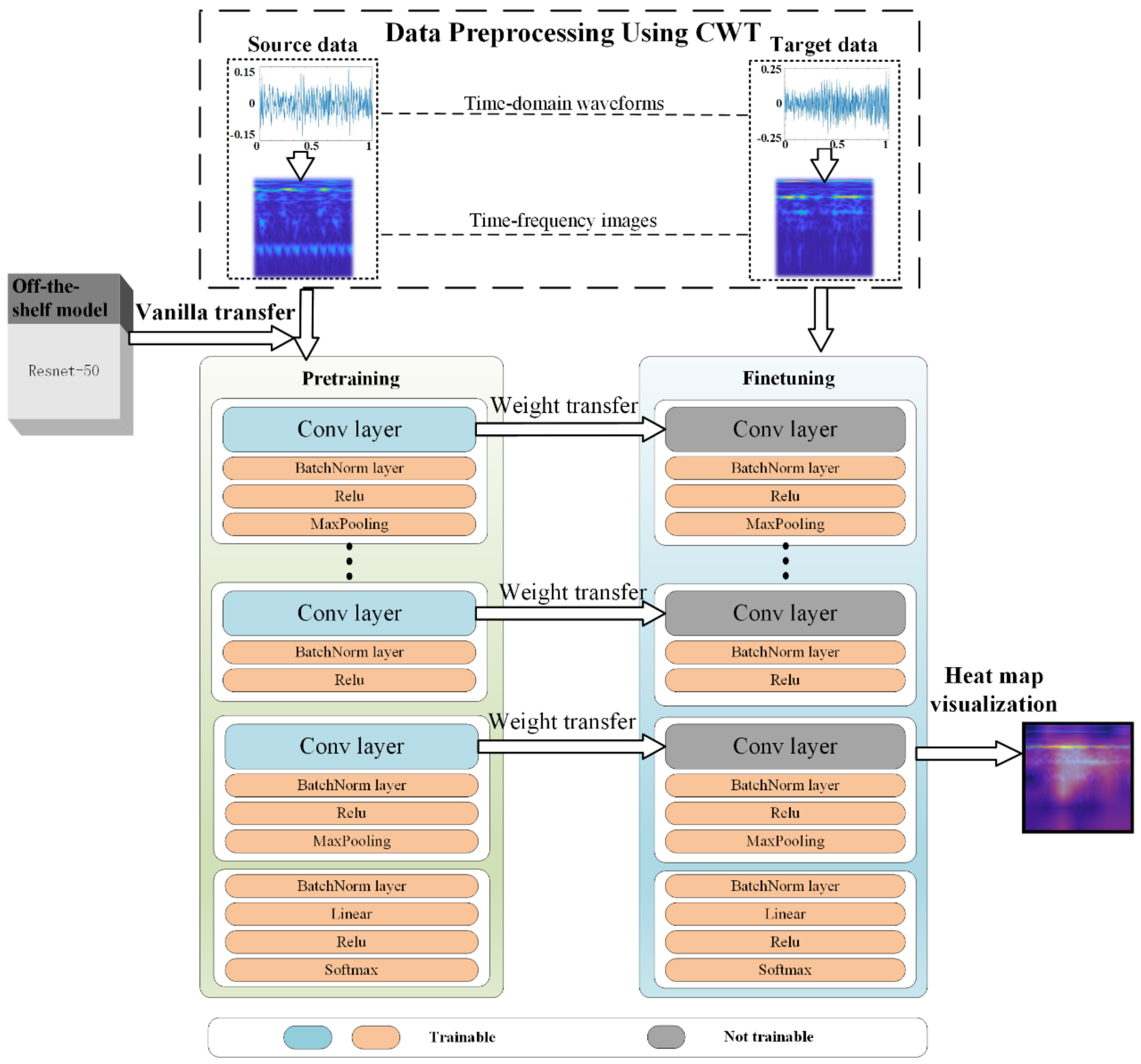
The intra-domain transfer learning strategy assumes the source domain is different from but akin to the target domain. Even so, negative transfer can still occur. To preclude this, we propose a two-stage transfer scheme: first, we construct a pre-trained model in the source domain via a vanilla transfer from an off-the-shelf inter-domain deep neural network; then, we transfer the pretrained model to the target domain via shallow-layer freezing and finetuning. Figure 2 depicts the two-stage intra-domain transfer learning strategy.

In our problem setting, the source domain is data-abundant, and this prevents negative transfer, even though we use an inter-domain vanilla transfer. We also use the first-stage transfer to speed up model training in the source domain. In the second stage, the shallow-layer freezing is intended to ensure knowledge transfer between akin domains, while finetuning uses the limited number of samples in the target domain to further train the model for better performance in target tasks.

In addition to requiring relative proximity between source and target domains, the intra-domain transfer learning strategy requires the source domain to be data-abundant. Note that in the field of fault diagnosis, annotated faulty samples are less expensive to acquire in the laboratory than in real-world applications. Therefore, a deluge of labelled samples in the source domain can be generated via fault injection experiments or simply first-principal simulation. This constitutes another motivation of this research.

2.2. Fault Diagnosis Model with Intra-Domain Transfer

Armed with the above intra-domain transfer strategy, in this section, we propose a fault diagnosis model for rotating machinery. Although many types of data (infrared images, temperature sequences, etc.) can be measured, vibration signals are still most prevalent in fault diagnosis applications. Without loss of generality, we assume both the source and the target domain use high frequency non-periodic vibration signals to diagnose faults.

Given their enormous capacity to represent knowledge, deep neural networks have been widely adopted as the carrier of knowledge in transfer learning applications. Specifically, convolutional neural networks (CNN) were early choices in the fields of computer vision and industrial fault diagnosis. Hereinafter, we use CNN as the main architecture for fault diagnosis modelling. Again, without loss of generality, we select ResNet-50 as our off-the-shelf inter-domain model since it is a benchmarking model [32]. Notably, the complexity (depth) of the selected model can vary depending on the problem to be solved, especially the complexity of the data input.

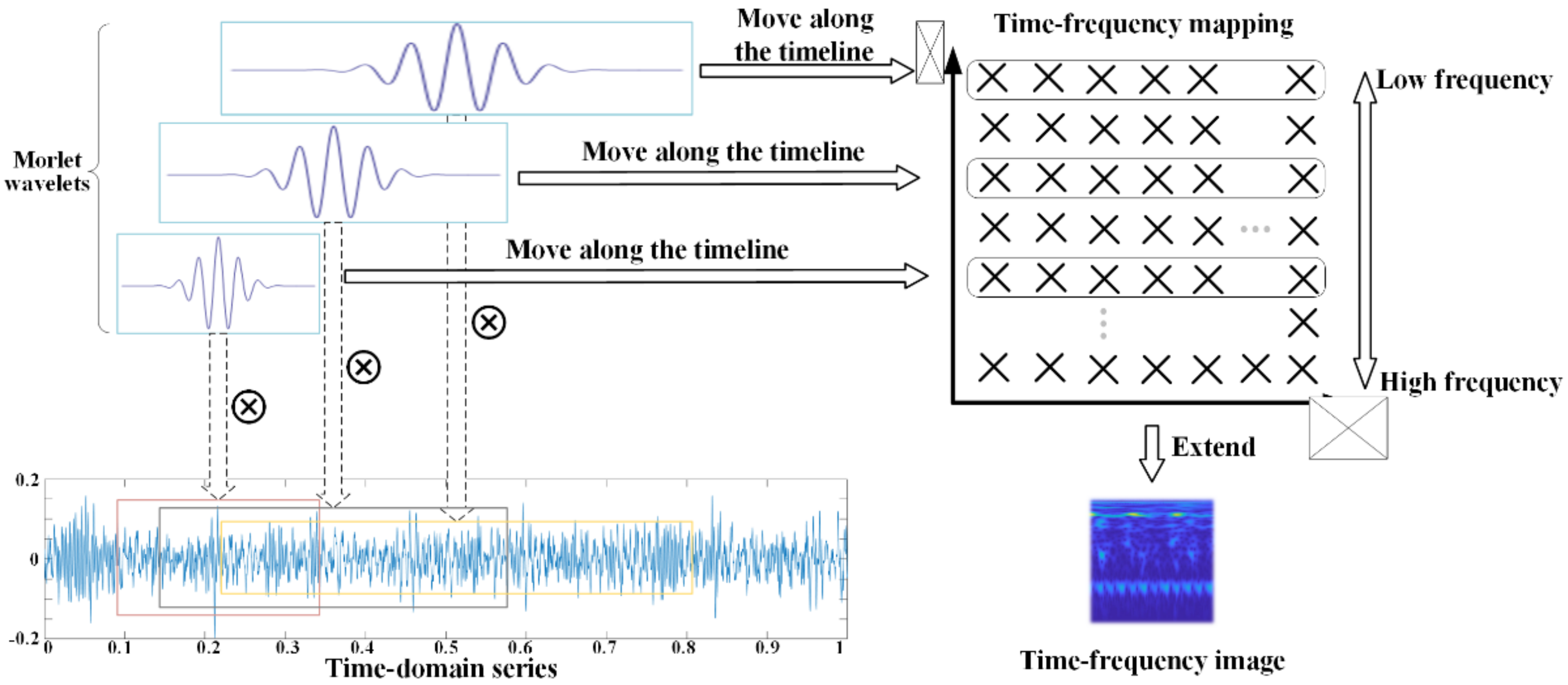
Since ResNet-50 is trained on natural images, we propose to use continuous wavelet transform (CWT) to convert our vibration signals to time-frequency spectrums, as has been carried out elsewhere [33]. This brings the data in source and target domains into the same format as the distant domain (i.e., images); see Figure 3 for an example. In addition, CWT conducts multi-scale transform on non-stationary signals, and this retains as much information as possible from the input. For simplicity, we select the complex Morlet wavelet as the mother wavelet, defined as:

$${\psi }_{a,\tau }\left(t\right)=\frac{1}{\sqrt{a}}\psi \left(\frac{t-\tau }{a}\right)$$

(1)

where $a$ represents a scale parameter related to frequency, and $\tau$ is a translation parameter related to time.

The wavelet coefficients of a signal are calculated by a convolution operation between the mother wavelet function ${\psi }_{a,\tau }\left(t\right)$ and the signal $x\left(t\right)$, as defined by:

$$W\left(a,\tau \right)=\frac{1}{\sqrt{a}}\int x\left(t\right){\psi }^{\ast }\left(\frac{t-\tau }{a}\right)dt$$

(2)

where ${\psi }^{\ast }\left(·\right)$ indicates the complex conjugate of function $\psi \left(·\right)$. The signal is decomposed into a series of complex numbers in distinct frequency bands, as shown in Figure 3. The moduli of the complex numbers are calculated and grouped by frequency and time. In this fashion, we get a one-dimensional signal mapping in the time-frequency domain, with the horizontal and vertical axes corresponding to time and frequency, respectively. Next, we conduct three-channel extensions of a time-frequency mapping to produce a time-frequency image.

The above time-frequency transformation describes the data preprocessing step of our fault diagnosis model. Once this step is completed, the model performs a vanilla transfer from ResNet-50 to the source domain. As the source domain is data-abundant, negative transfer in this step can be avoided. Studies in computer vision have found the convolutional layers of a CNN are essential for automatic feature learning. The deeper the layers, the more abstract the learned features are, and vice versa.

That being said, we propose shallow-layer freezing to ensure feature extractors in the source domain are reused in the target domain. The sharing of feature extractors is supported by assuming the distribution discrepancy between source and target domains is reasonably small. In other words, the weights of those shallow layers in the CNN are fixed to extract features in the target domain (i.e., features shared in common with the source domain).

The last step of our fault diagnosis model is finetuning in the target domain. Concretely, the final classification layer (e.g., a soft-max layer) of the CNN is customized to fit the number of classes in the target domain. Those learnable weights in the deep layers are further trained using the small samples to accomplish the target task. The finetuning step aims to improve the generalization capability in the target task, and it is typically implemented at a small learning rate, depending on the number of samples available. A summary of the above steps appears in Figure 4.

3. Experiments and Results

To validate the proposed intra-domain transfer learning strategy and the fault diagnosis model, we select a bearing dataset and a gearbox dataset for a case study comparing various transfer strategies. We also carry out extensive experiments to empirically analyze the impact of training sample scarcity on diagnostic accuracy.

3.1. Dataset Introduction

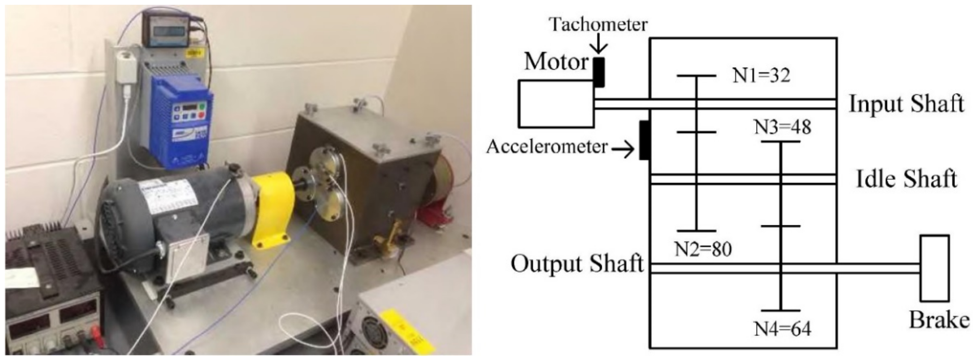
The gearbox dataset, featuring small samples in the target domain, was collected from a two-stage gearbox test rig, as shown in Figure 5. Vibration signals of the gear were measured via an accelerometer attached to the gearbox housing. The signals were recorded using a dSPACE system (DS1006 processor board, dSPACE Inc., Wixom, MI, USA) at a sampling frequency of 20 kHZ. 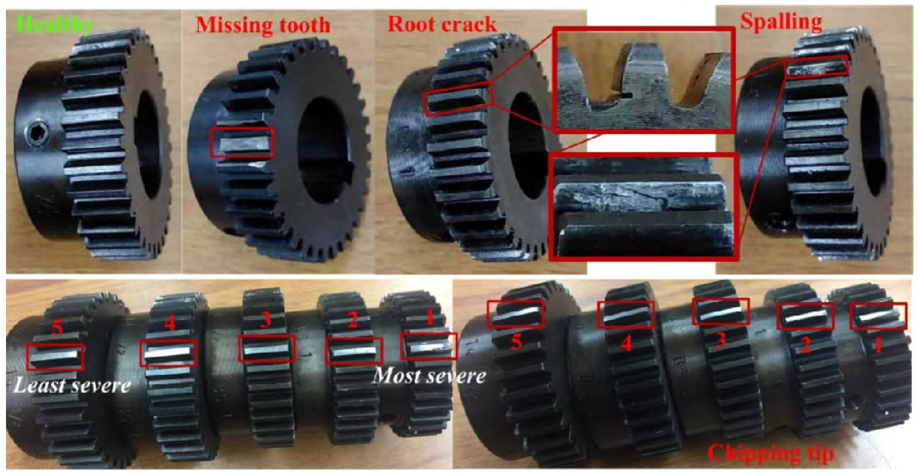More details about the test rig and data acquisition apparatus are in [8]. The dataset was gathered under nine working conditions: healthy, missing tooth, root crack, spalling, and chipping tip with five different severities. These conditions are shown in Figure 6.

Each working condition of the gearbox dataset has 104 samples, each of which has a length of 3600.

Table 1. Metadata of the gearbox dataset.

Working Conditions	Sampling Frequency (HZ)	Number of Samples	Length of Each Sample
Healthy	20k	104	3600
Missing	20k	104	3600
Crack	20k	104	3600
Spalling	20k	104	3600
Chip5a	20k	104	3600
Chip4a	20k	104	3600
Chip3a	20k	104	3600
Chip2a	20k	104	3600
Chip1a	20k	104	3600

briefly describes some metadata of the dataset. In the case of a nine-class classification problem where the number of samples is far less than the sample dimension, it is challenging to train a reasonably good diagnostic model from scratch. In addition, fault signatures might be submerged by meshing frequencies and noises, thus aggravating the difficulties of feature extraction. Note that when the dataset was released originally in [8], the authors considered utilizing transfer learning to solve the problem, but ultimately chose a different approach.

The Case Western Reserve University (CWRU) bearing dataset is chosen as the source domain for transfer learning in this study, as it is one of the most extensively used datasets for fault diagnosis benchmarking [34]. The dataset contains vibration signals collected at a frequency of 12kHz and 48kHz. We only utilize those with a sampling frequency of 12 kHz to reduce variation in the source domain. Three types of faults (ball, inner race, and outer race) are introduced in the experiments, each with three fault sizes (0.007, 0.014, and 0.021 in).

The monitoring items, sampling frequency, and working conditions are different across source and target domains, but both datasets have high-frequency aperiodicity. Moreover, the source and target domains resemble each other visually after time-frequency transformation, allowing us to transfer feature extractors between intra-domains.

3.2. Data Preparation

Following the proposed fault diagnosis model in Section 2, we convert the time-domain waveforms of the source and target domains into time-frequency images using CWT. Under the condition that Nyquist’s sampling theorem is satisfied, the waveforms are first sliced into vibrational snippets of equal length, 1200 points in our experiments. Each vibration snippet is transformed into one time-frequency image of size 224 × 224 via down-sampling. The images are then extended to three channels to fit the input dimension of ResNet-50. 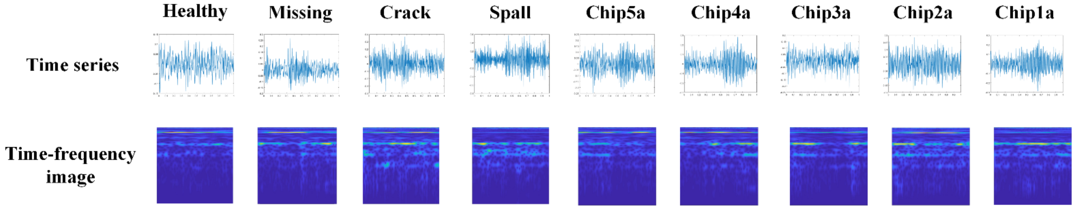Figure 7 shows an example of the time-frequency images in our target domain.

Using the above approach, we construct two data repositories of time-frequency images: one is the source-domain CWRU dataset for pretraining; the other is the target-domain gearbox dataset for finetuning and model validation. The former consists of nine faulty states (three fault locations and three sizes), each of which has 1203 time-frequency domain images; approximately 20% of them (240) are used for model selection. The latter has 2808 samples, and each of the nine working conditions includes 312 samples. To investigate how the number of samples in the target domain affects the diagnostic accuracy, we split the target domain into a training set and a testing set using different ratios: 90:10, 50:50, 10:90, 5:95, and 1:99. This is summarized in

Table 2. Target-domain training/testing set division under different splitting ratios.

Splitting Ratios	Total Number of Samples	Number of Samples for Each Working State
		Training Set	Testing Set
90:10	2808	2529	279
50:50	2808	1404	1404
10:90	2808	279	2529
5:95	2808	144	2664
1:99	2808	27	2781

.

3.3. Pretraining and Finetuning

To validate the intra-domain transfer learning strategy and the proposed fault diagnosis model, we introduce two more learning schemes for comparison: train from scratch (TFS) and transfer from ImageNet (TFI). The proposed intra-domain transfer learning method is abbreviated as TFC, signifying transfer from the CWRU dataset.

The weights of the ResNet-50 model are randomly reinitialized in TFS. We can imagine the dilemma the TFS scheme ran into with small samples to train such a complex model. All of the convolutional layers of TFI and TFC inherit weights from the off-the-shelf ResNet-50 model, and their batch normalization layers and the fully-connected layers are reinitialized.

With prior knowledge that the target-domain samples differ significantly from natural images, the convolutional layers of TFI are trainable but at a relatively small learning rate. Therefore, the convolutional layers of TFC are frozen to reuse the feature extractors learned from intra-domain samples. The final soft-max layer of each of the above three schemes is customized to match the number of desired classes in our target task. We choose Adam optimizer in our pretraining and finetuning, and the learning rate is set to 1 × 10⁻⁴. All models are trained with mini-batch samples of a size of 16.

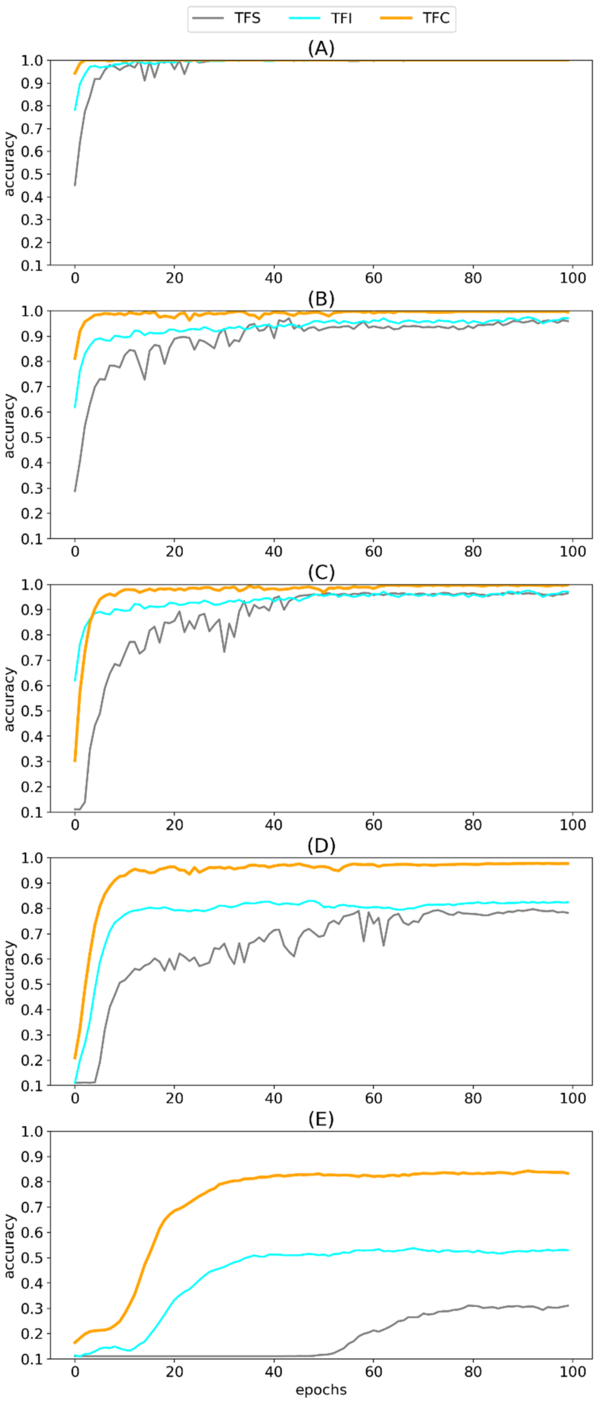
Under the settings of the three training schemes and five splitting ratios of target-domain samples, we train the ResNet-50 model for 100 epochs, each repeated five times. The training history is shown in Figure 8. From the figure, we observe the proposed method converges faster than the alternatives, and it consistently plateaus at the highest diagnostic accuracy in our target task. Given adequate training samples, all three learning schemes can achieve a satisfactory result if the model is sufficiently trained. But when training samples are scarce, intra-domain transfer learning can boost the performance in terms of both convergence speed and accuracy in the target task.

3.4. Testing Resultss

Testing accuracy of the three learning schemes in our target task is shown in

Table 3. Testing accuracy in the target task under three learning schemes and various splitting ratios of target-domain samples (each number is an average of five runs of experiments).

Learning Schemes	Best Accuracy in First 10 Epochs (%)					Best Accuracy in First 50 Epochs (%)					Best Accuracy in First 100 Epochs (%)
	90:10	50:50	10:90	5:95	1:99	90:10	50:50	10:90	5:95	1:99	90:10	50:50	10:90	5:95	1:99
TFS	97.1	82.4	72.5	51.6	11.1	100	97.0	89.2	69.2	11.6	100	97.0	96.6	79.0	33.6
TFI	98.9	90.1	92.2	74.5	14.9	100	97.9	97.2	82.9	51.2	100	99.0	97.5	82.3	53.1
TFC	100	99.0	97.8	92.9	27.9	100	99.5	98.9	97.5	83.2	100	99.8	99.7	97.8	84.3

. The proposed intra-domain transfer learning strategy exhibits the best diagnostic accuracy, even with small training samples. With proper model training, TFS can achieve a high prediction accuracy in the testing set when training samples are abundant, but it degenerates as the number of training samples decreases. In general, TFI improves the performance compared to TFS, indicating that inter-domain experience helps classify faults in the gearbox dataset. But as shown in Figure 8B,C, negative transfer does occur occasionally, though this is not always evident.

As shown in Figure 8 and Table 3, TFC (the proposed learning scheme) consistently outperforms TFI. There is a large gain in accuracy using intra-domain transfer instead of its inter-domain counterpart. This confirms that the feature extractors learned from a different but akin domain can not only avoid negative transfer but also boost prediction accuracy in the target task. Table 3 also demonstrates that TFC has strong generalization capability even when the splitting ratio is set to 1:99, resulting in an accuracy of 84.3% after 100 epochs of training. We note that a nine-class classification problem is not an easy task.

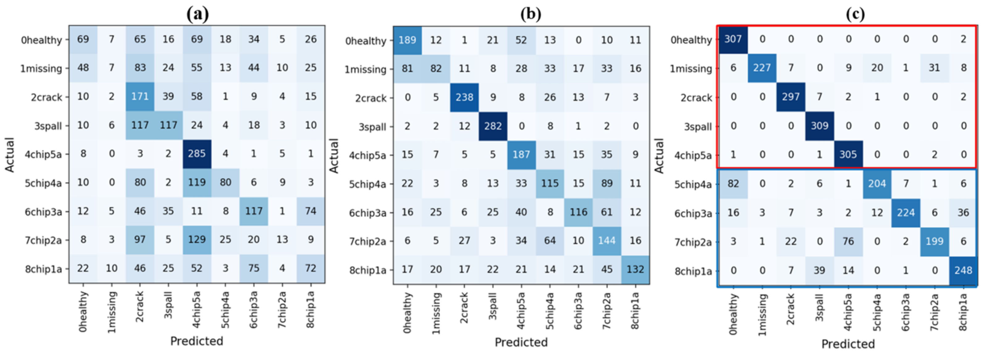
The confusion matrices of the three learning schemes with small training samples are shown in Figure 9. As the figure indicates, TFS performs slightly better than random guessing, and the most misclassified classes are “chip4a” and “chip2a”. TFI obtains a higher diagnostic accuracy, and misclassifications distribute more evenly across different classes. TFC significantly improves the classification of “healthy”, “missing”, “crack”, “spall”, and “chip5a”, leading to an accuracy of 93.5% in these five states (red rectangle). The remaining four states (blue rectangle) have a relatively higher misclassification rate. An intuitive explanation is that the four faults are of the same type but have different severities. Consequently, their features are comparable, making it hard to distinguish them. Although data size considerably affects the diagnostic accuracy, the proposed method can achieve satisfactory results when training samples are scarce. This proves the efficacy of using the intra-domain transfer learning strategy for fault diagnosis with small samples.

4. Demystifying the “Black-Box” via Visualization

This section adopts the heat map method to demystify the learned fault diagnosis model, giving us a way to visualize high-level features of inputs in an intuitive and explainable manner. As a complementary study to the proposed intra-domain transfer learning strategy, we compare the above three learning schemes via heat map visualization.

4.1. Heat Map Visualization

Heat mapping is widely used in computer vision applications [35,36]. It attempts to visualize the most activated area in an input to reveal how the final classification conclusions are drawn by deep learning models. For example, in a face recognition problem, those image patches corresponding to noses, eyes, and mouths will contribute the most to the final decision. Similarly, we hypothesize that fault-related frequencies in our time-frequency images should be recognized by our ResNet-50 model in the target task.

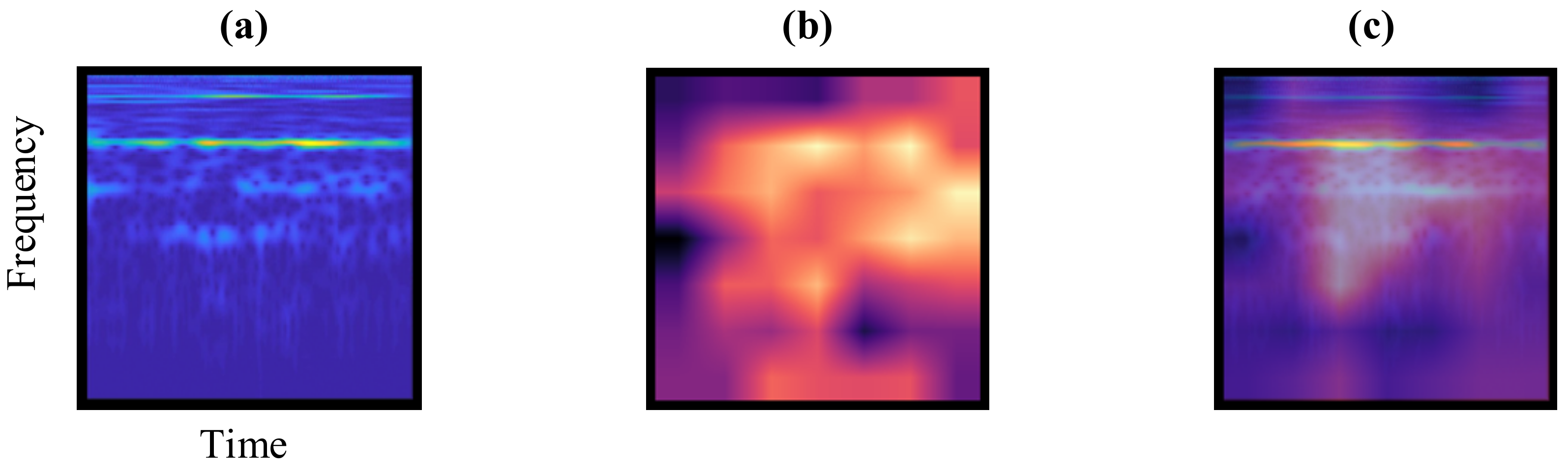
The deeper the layer in a model, the more abstract the extracted features. Therefore, we use the feature maps yielded by the last convolutional layer of the ResNet-50 model to construct a heat map. In the ResNet-50 architecture, the output size of the last convolutional layer is 512 × 7 × 7, corresponding to channels, heights, and widths, respectively. Taking the average along the first axis produces a 7 × 7 matrix. Note this channel-wise average operation is different from the average pooling layer in the ResNet-50 model, as it averages over the whole feature map.

The magnitude of the above matrix reflects the extent of the activation in the original input but on a much smaller scale. To solve this, we up-sample the matrix to match the input size using bilinear interpolation; this results in an average activation matrix, as shown in Figure 10b. We select bilinear interpolation to make the transition between image blocks smoother. Then, the final heat map can be obtained by overlaying the average activation matrix on the original input. Figure 10 demonstrates an example of heat map visualization taking a time-frequency image of our target sample as input.

4.2. Qualitative Assessment of the Heat Maps of the Target Task

The ability to learn high-level abstraction of features using CNN has already been verified in computer vision applications but is relatively underexplored in fault diagnosis. Armed with the above heat map method, we attempt to visualize those high-level features extracted by the transferred ResNet-50 model in our target task and correlate them with the underlying fault characteristics. Hereinafter, to validate the efficacy of our proposed intra-domain transfer learning strategy using small samples, we analyze the model finetuned when the splitting ratio of training and testing samples is set at 1:99.

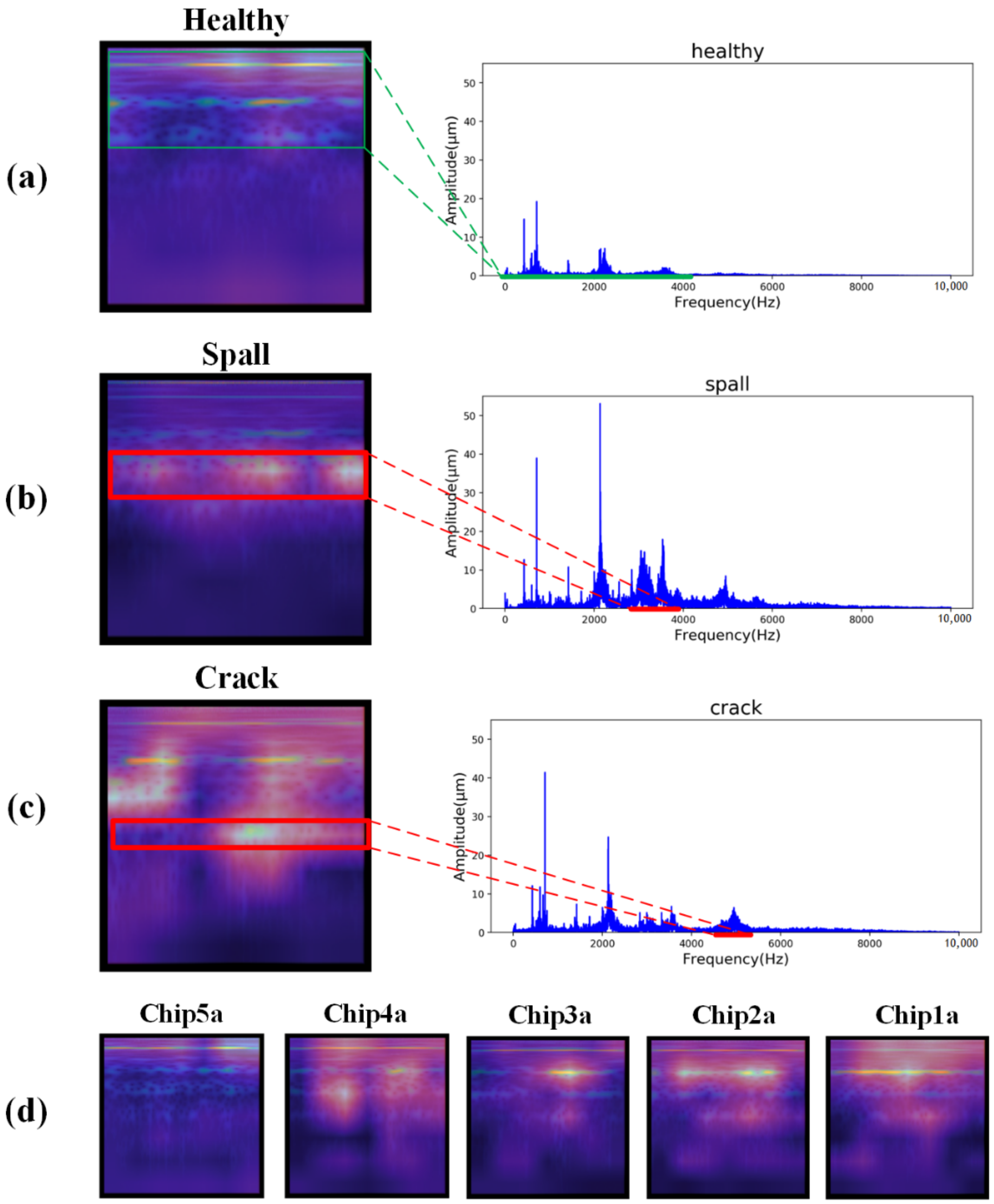
Figure 11 shows some heat maps generated by the fault diagnosis model at testing time. Each heat map corresponds to one random testing sample in a specific working condition in our target task; see Table 1 for a reference. Three frequency spectrums are presented in Figure 11. Healthy samples are normally characterized by an amplitude located at the shaft rotating frequency and its harmonies, as shown in Figure 11a, while faulty samples can be recognized by anomalous amplitude in their characteristic frequencies.

The activations highlighted in red boxes are consistent with their corresponding fault characteristics. For example, as shown in the frequency spectrum of Figure 11c, the fault “crack” has a characteristic frequency around 5000 Hz, and the energy in this frequency band is correctly identified in its heat map. Similar results can be observed in other fault classes. Notably, the horizontal axis in our heat map is time, the same as in the time-frequency image. Therefore, the horizontal location of the most activated area can also signify the temporal features of non-stationary signals that lead to CNN’s final classification.

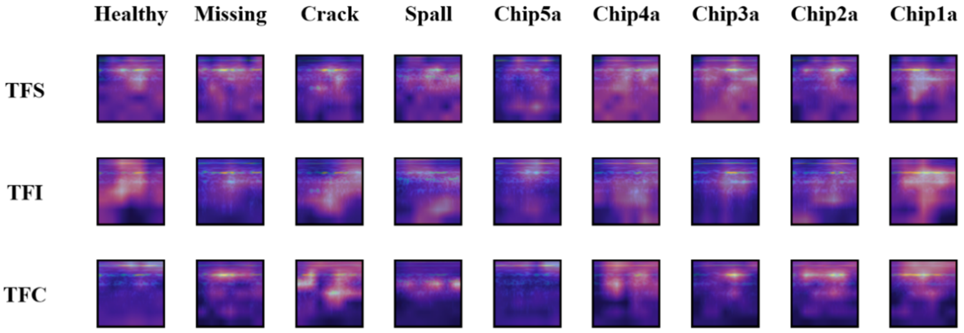
Another observation is the most activated spots in these heat maps are distinctive, making it easy to separate them. Figure 12 compares the heat maps of the various working conditions obtained via the three learning schemes. Intuitively, it can be deduced that TFC leads to the highest differentiability in these heat maps, TFI ranks second, and TFS comes in last. This coincides with the confusion matrices shown in Figure 9 and the testing accuracy results in Table 3.

From a result-oriented perspective, higher differentiability in the heat maps would yield higher diagnostic accuracy. But it by no means implies that the most activated area in the feature maps must match the underlying physical mechanisms of the corresponding faults. The above qualitative assessment of the heat maps not only proves the efficacy of the proposed intra-domain learning strategy, but also discloses how the transferred ResNet-50 model infers the diagnostic results. Since the feature extractors learned from an intra-domain task are frozen in our target-domain task, the knowledge sharing enabled by our transfer learning strategy is validated in the heat maps. Moreover, the heat maps of misclassification samples can provide new perspectives to improve the fault diagnosis model.

5. Conclusions

This study proposed an intra-domain transfer learning strategy to tackle the challenge of insufficient training samples in fault diagnosis applications. To alleviate the impact of negative transfer, the intra-domain transfer learning strategy first uses the vanilla transfer of an off-the-shelf inter-domain model to a data-abundant source domain that is akin to the target domain. The learned feature extractors are then reutilized in the target domain via shallow-layer freezing, followed by a finetuning step with small samples.

We verified the proposed transfer learning strategy in a gearbox fault diagnosis case study and compared it to two other learning schemes. In the case study, we adopted CWT as a preprocessing tool to convert 1D vibrational waveform to 3D time-frequency images, and selected ResNet-50 as the base model. Under various small sample settings (splitting ratio of training and testing samples in the target task), we carried out extensive experiments and observed superior performance of the proposed strategy in both convergence speed and accuracy. Finally, we introduced heat map visualization to demystify the learned deep neural network. We leave the quantitative assessment of a fault diagnosis model using heat maps to future work.