Time Series Recovery Using Adjacent Channel Data Based on LSTM: A Case Study of Subway Vibrations

Abstract

Multi-sensor technology has been widely applied in the condition monitoring of rail transit. In practice, the data of some channels in the high channel counts are often abnormal or lost due to the abnormality and damage of the sensors, thus resulting in a large amount of data waste. A method for the data recovery of lost channels by using adjacent channel data is proposed to solve this problem. Based on the LSTM network algorithm, a data recovery model is established based on the “sequence-to-sequence” regression analysis of adjacent channel data. Taking the measured vibration data of a subway as an example, the network is trained with multi-channel measured data to recover the lost channel data of time-series characteristics. The results show that this multi-channel data recovery model is feasible, and the accuracy is up to 98%. This method can also further reduce the number of channels that need to be collected.

1. Introduction

With the continuous development of urban rail transit, subway lines have developed rapidly in many cities. With the increasing demand for transportation facilities construction, a large amount of measured data in terms of subway evaluation, field testing, experimental verification, and simulation have been collected. Due to the sensor used for data acquisition being affected by vibration, some sensors are damaged, and the data is lost during the collection process, leading to a large amount of data waste. The data waste can be significantly reduced if the lost data can be recovered based on the existing normal data from adjacent channels.

Research on lost data recovery is usually based on historical data to build a data recovery model [1]. At present, the research methods for data recovery can be roughly divided into three categories: The first is traditional mathematical models, including the moving average method, historical trend method, residual grey model, and interpolation method [2,3,4,5,6]. The second is intelligent recovery methods, including nonparametric regression and neural networks [7,8]. The third is combination models [9,10], which refers to a combination of two or more data processing methods. Although conventional methods can achieve the accurate recovery of single missing datasets, important information in long-term time series data is often ignored in addition to a prolonged estimation time, which causes missing data and distortion and has a greater impact on subsequent data analysis. The intelligent recovery method, especially the use of a neural network, can identify the characteristics, trends, and development laws of the variable changes from the time series, thereby achieving the effective prediction and recovery of the missing data. The intelligent recovery method mainly employs machine learning algorithms to identify and recover abnormal and lost data, and it is currently widely used for data recovery.

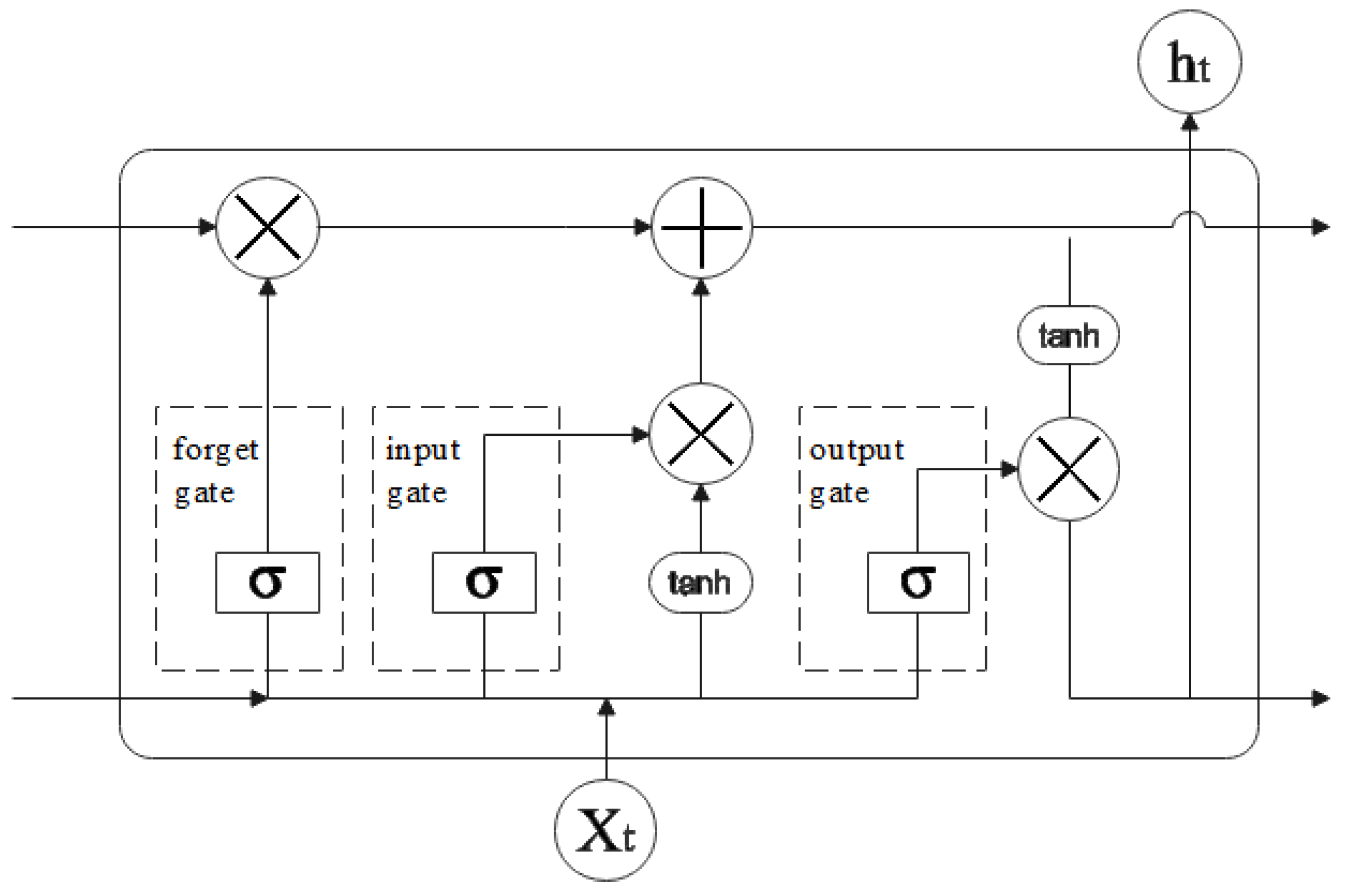
With the advancement of machine learning, it is possible to predict future multi-epoch data by quantifying the relationship between current data and historical data through the characteristic trend in the data over time. Kamat et al. and Sanakkayala et al. [11,12] tried to use deep learning to monitor abnormal bearing data, and the results showed that deep learning achieved very high accuracy and robustness in monitoring the future state of things with the historical data. As the data have characteristics in the format of time series, learning temporal dependencies from sequence data poses challenges to classical machine learning techniques and standard neural networks. The long short-term memory (LSTM) network addresses this problem by introducing memory units into the network architecture. The LSTM network has great advantages in analyzing large-scale data [13,14], and it has high prediction accuracy for time-series data such as atmospheric and ocean temperature, traffic flow, and vibration signals [15,16]. For example, Milad et al. applied the LSTM model to the temperature prediction of pavement roads [17]. Based on the excellent performance of the LSTM model, Li et al. [18] considered the influence factors of historical air quality and meteorological data and realized the fast and accurate prediction of PM2.5 by analyzing the long-term historical process of time-series data. Han et al. [19] applied a one-dimensional convolutional neural network (1-D CNN) and an LSTM to analyze vibration signals for bearing fault diagnosis. Ma et al. [20] proposed a CNN-LSTM model for the accurate point-by-point prediction of high-speed railway car body vibration. LSTM networks perform well in extracting knowledge from sequence data over time spans, as has been shown in previous studies. Nowadays, an LSTM neural network is mainly used for the prediction of single-channel time-series data based on historical data. However, in a scenario where multi-channel data is collected, especially when there is a certain correlation of data between channels, there is inadequate research on the use of neural networks in which the complete data of multiple channels is used for restoring missing data on a neighboring channel. The accuracy of recovering the data of one channel using neighboring channels should be further studied. To be specific, a set of data from a total of eight channels was collected, but the data from Channel 7 were missing. Then, the neural network was used to train the remaining complete data of multiple channels, thus recovering the missing data of Channel 7.

2. LSTM Neural Network Modeling

In this study, an LSTM neural network is proposed to analyze time-series data based on the characteristic trend of multi-channel data collected over time.

2.1. LSTM Basic Algorithm

A traditional RNN network can retain the effective information of the previous sequence samples and impact the current output. However, traditional RNN network training often has the phenomenon of gradient disappearance or gradient explosion when processing long input sequence samples, resulting in a poor network training effect. To solve this problem and improve the performance of an RNN network, some scholars have introduced gate operations on the hidden layer nodes of a traditional RNN network, resulting in some RNN variants, such as an LSTM network and a gated recurrent unit (GRU) network [21,22,23]. In practice, LSTM networks have achieved good results. An LSTM network can selectively memorize sequence information, with advantages such as the satisfactory applicability to measurement data, high accuracy, and short response time. The research of Zhen et al. [24] proved that the recognition rate of LSTM neural networks in diagnosis of different faults of a single or multiple sensors is over 96% and that the response time is less than 1 millisecond. Wang et al. [25] applied an LSTM to the fault detection and recovery of UAV flight data, and they found that satisfactory performance was achieved. Three types of gates in LSTM networks are as follows: input gate, forget gate, and output gate. It is possible to control the flow of information between the hidden layers of an LSTM network by adjusting the state of these gates. The hidden layer of the original RNN has only one state and is very sensitive to short-term inputs. An LSTM adds one cell state to the RNN to keep the long-term state. An LSTM neural network structure is shown in Figure 1.

The forget gate f_t determines the degree to which the long-term characteristics of preorder information are preserved or discarded in the cell state, which can be expressed as:

$$\mathsf{\mu }=\frac{1}{m}{\displaystyle \sum }_{i=1}^m{x}_i$$

where f_t is the activation value of output h_t−1 at t − 1, the input value at t, and the bias term of b_f. The function is sigmoid, and f_t is scaled down between zero (complete forgetting) and one (complete memory). W_f is the weight term and includes W_fx and W_fh.

The input gate determines how to update the cell state, namely, the new information is selectively memorized to the cell state C_t. The formula is as follows:

$$\{\begin{array}{c}{i}_t=\sigma \left(W_i·\left[h_{t-1},x_t\right]+b_i\right)\\ {\tilde{C}}_t=\mathrm{t}\mathrm{a}\mathrm{n}h \left(W_C·\left[h_{t-1},x_t\right]+b_C\right)\\ C_t=f_t{}^{*}{C}_{t-1}+i_t{}^{*}{\tilde{C}}_t\end{array}$$

where h_t−1 and x_t are passed to the sigmoid function to obtain its value; h_t−1 and x_t are passed to the tanh activation function to obtain the candidate value ${\tilde{C}}_t$ of the cell state, and it and ${\tilde{C}}_t$ jointly determine the new cell state; W_i, and W_C are weight terms, including W_ix and W_ih and W_Cx and W_Ch, respectively; b_i and b_C are bias terms; and “*” refers to multiplication with matrix elements.

The output gate O_t determines the input at the present moment. Similar to the input gate, the information carried by h_t is determined by O_t and C_t, and the formula is as follows:

$$\{\begin{array}{c}{O}_t=\sigma \left(W_O·\left[h_{t-1},x_t\right]+b_O\right)\\ h_t=O_t{}^{*}\mathrm{t}\mathrm{a}\mathrm{n}h\left(C_t\right)\end{array}$$

where W_O is the weight term, which includes W_ox and W_ho, and b_O is the bias term.

The LSTM method diagram is shown in Figure 2.

2.2. Sample Data Normalization

In order to make the data more convenient for processing with the model and avoid the influence of different dimensions between each feature and the target value on the prediction performance, as well as to speed up the gradient descent, the Z-score method is used to normalize the sample data, where the training predictor variable is normalized into a variable with a zero mean and unit variance. The main steps are as follows:

1.

Obtain the mean μ of the output data x as Equation (1):

$$\mathsf{\mu }=\frac{1}{m}{{\displaystyle \sum }}_{i=1}^m{x}_i.$$

(1)

2.

Obtain the variance σ of the output data as Equation (2):

$${\sigma }^2=\frac{1}{m}{{\displaystyle \sum }}_{i=1}^m{\left(x_i-\mathsf{\mu }\right)}^2.$$

(2)

3.

Obtain the output data normalization as Equation (3):

$$x_i=\frac{x_i-\mu }{\sqrt{{\sigma }^2}},$$

(3)

where m represents the number of samples in one batch of the input batch training and x_i represents the input value of sample i.

2.3. Evaluation Index

In this paper, the root mean square error (RMSE) and mean absolute error (MAE) evaluation indicators are used to aid the evaluation of the restoration effectiveness of the abnormal data. The foregoing means the deviation between the restored value and true value, reflecting the restoration capacity. The lower the error value, the better the restoration effect and the higher the accuracy of the restored data. At the same time, the coefficient of determination R² is adopted to evaluate the effectiveness of the model. The coefficient of determination R² is a value between zero and one. The closer it is to zero, the poorer the fitting effect of the prediction model for the real data, and the closer it is to one, the better the fitting effect of the prediction model for the real data. The calculation formula is:

$$\mathrm{RMSE}=\sqrt{\frac{{{\displaystyle \sum }}_{i=1}^n{\left(v_r-v_c\right)}^2}{n}},$$

(4)

$$\mathrm{MAE}=\frac{1}{N}{{\displaystyle \sum }}_{i=1}^N\left|y_i-{\widehat{y}}_i\right|, \mathrm{and}$$

(5)

$$R^2=1-\frac{{{\displaystyle \sum }}_{i=1}^N{(y_i-{\widehat{y}}_i)}^2}{{{\displaystyle \sum }}_{i=1}^N(y_i-\overline{y}{)}^2},$$

(6)

where v_c is the real value, v_r is the restored value, and n is the amount of data.

3. Case Study

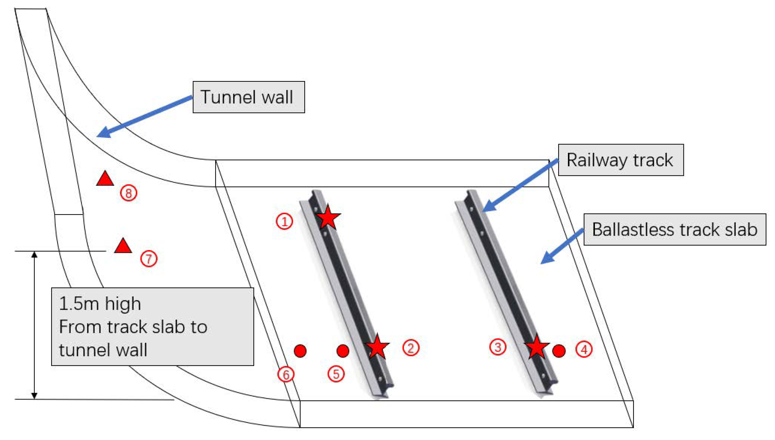
Taking the vibration and noise level test in a subway tunnel as an example, INV3062V network distributed acquisition instrumentation and LC0161BG piezoelectric acceleration sensors are used for the data acquisition, with a frequency response of 0.1–1000 Hz, a measuring range of 5 g, and a testing accuracy of 0.0002 g. The arrangement of measuring points is shown in Figure 3. The measuring points of the tunnel section are arranged and include the rail, the track slab, and the tunnel wall. Eight channel data are selected, and each channel has 12,800 sampling points for analysis to ensure the validity of the network model.

In order to verify the accuracy of this prediction model, two different data processing methods will be used to predict the missing channel data. The first method is to directly train and verify the neural network with the raw data (time-domain data) collected by sensors. The second method is to perform a Fourier transform on the original data (frequency domain data) and then use the transformed data to train and verify the neural network.

3.1. Training the Network with Time-Domain Data

3.1.1. Neural Network Training Process

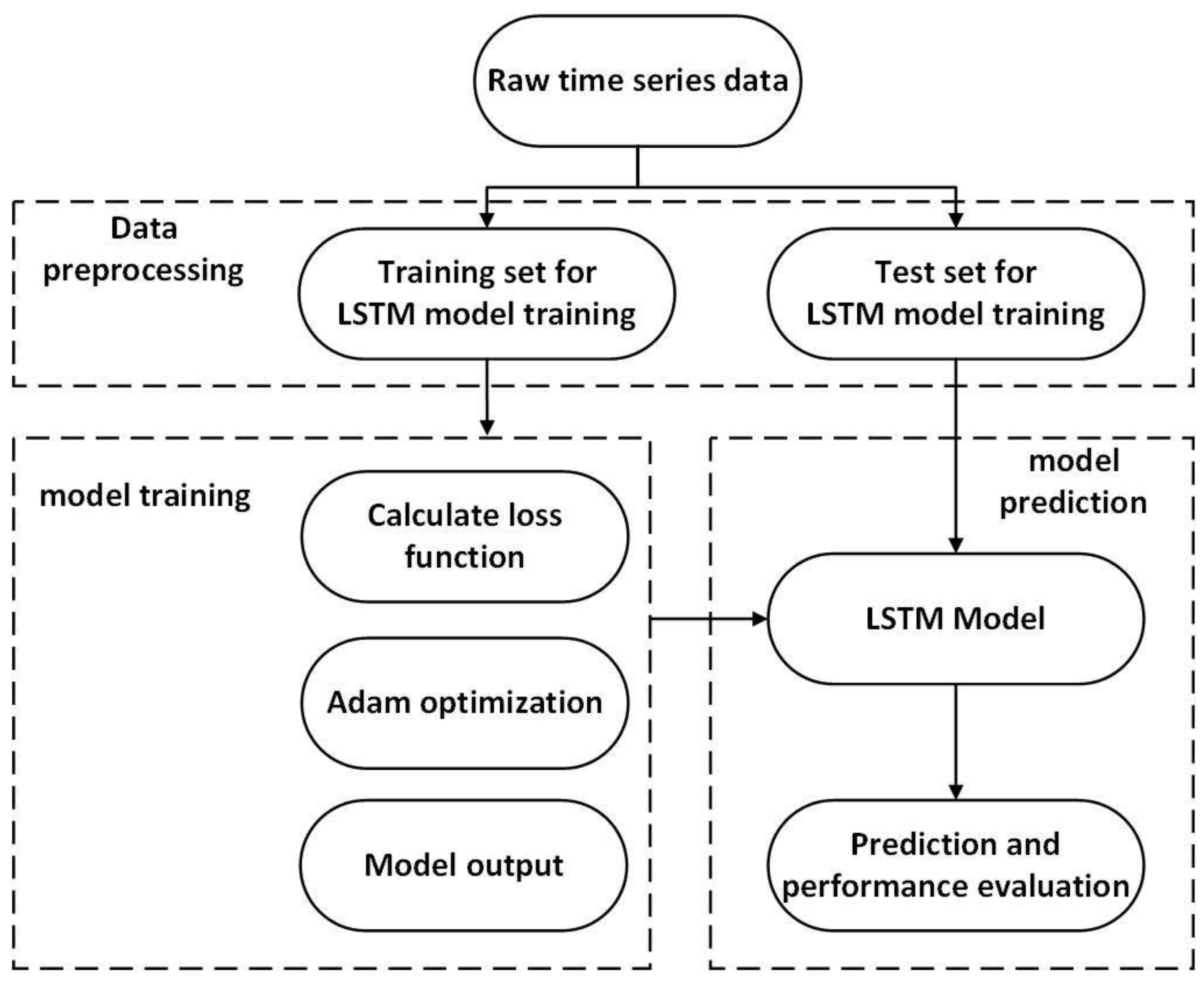
This study builds a multi-channel data recovery model and defines the network architecture. The LSTM network that contains an LSTM layer with a specified number of hidden units and a fully connected layer is created. The solver ‘Adam’ is used to train epochs and batch size based on user-specified size. The learning rate is specified as 0.03.

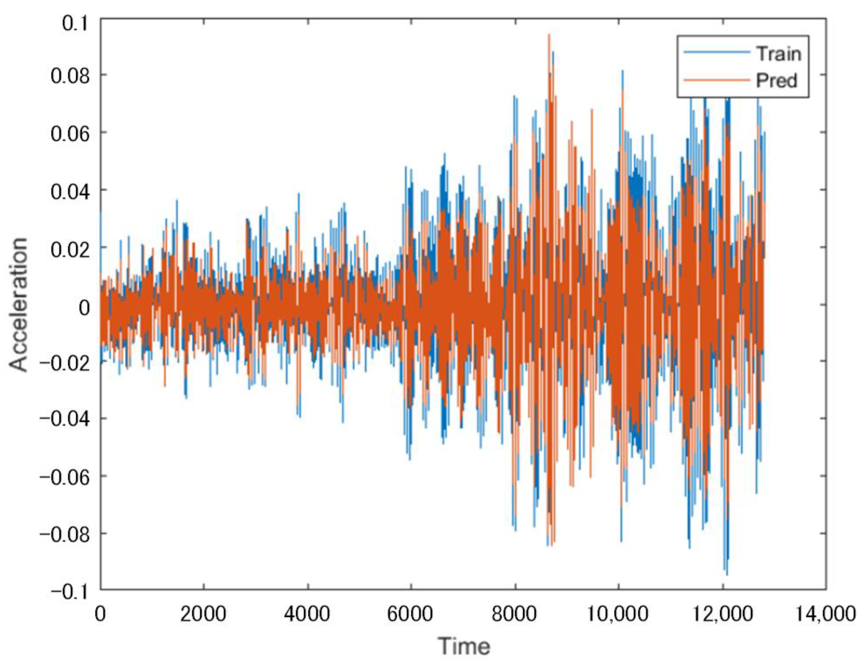
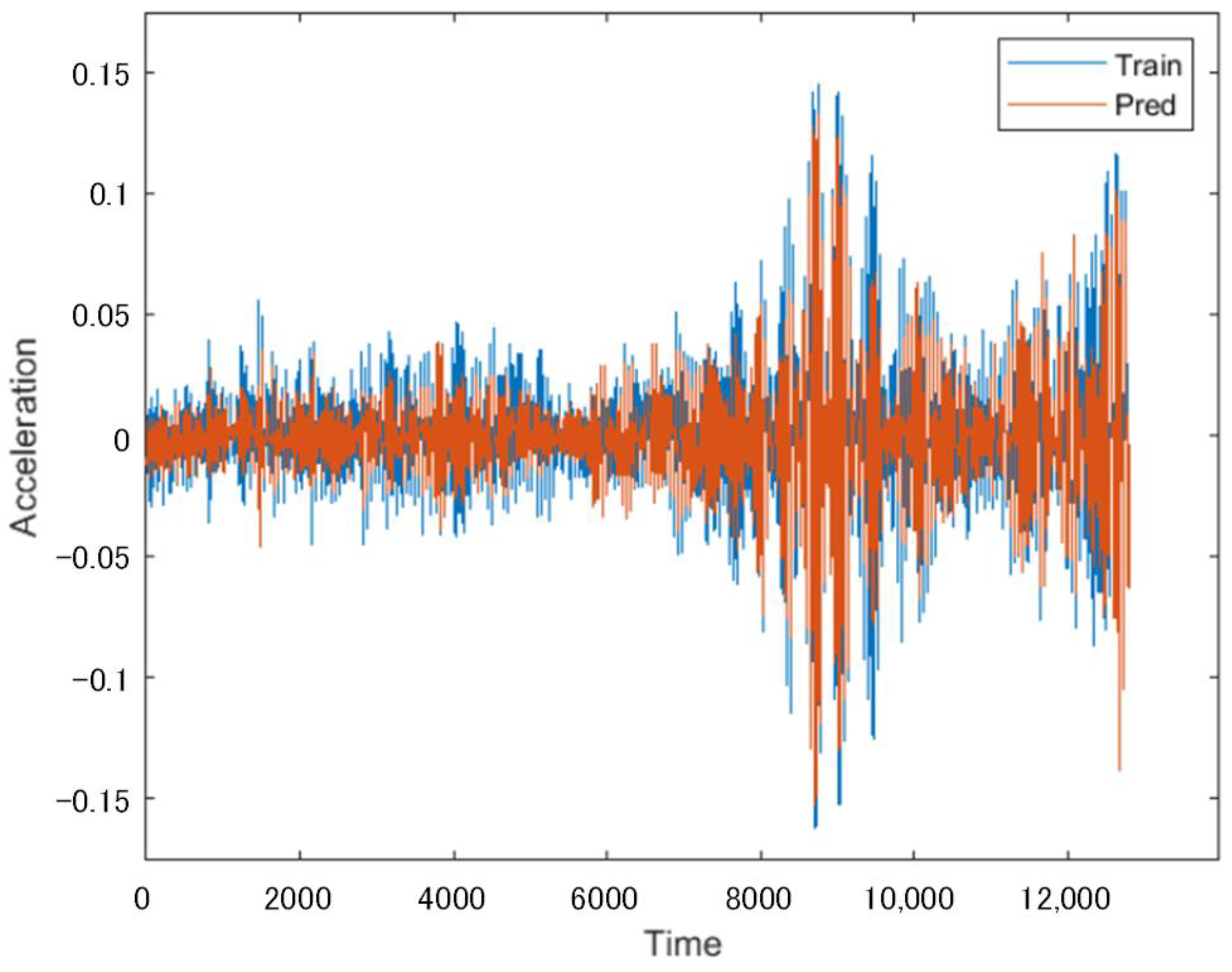
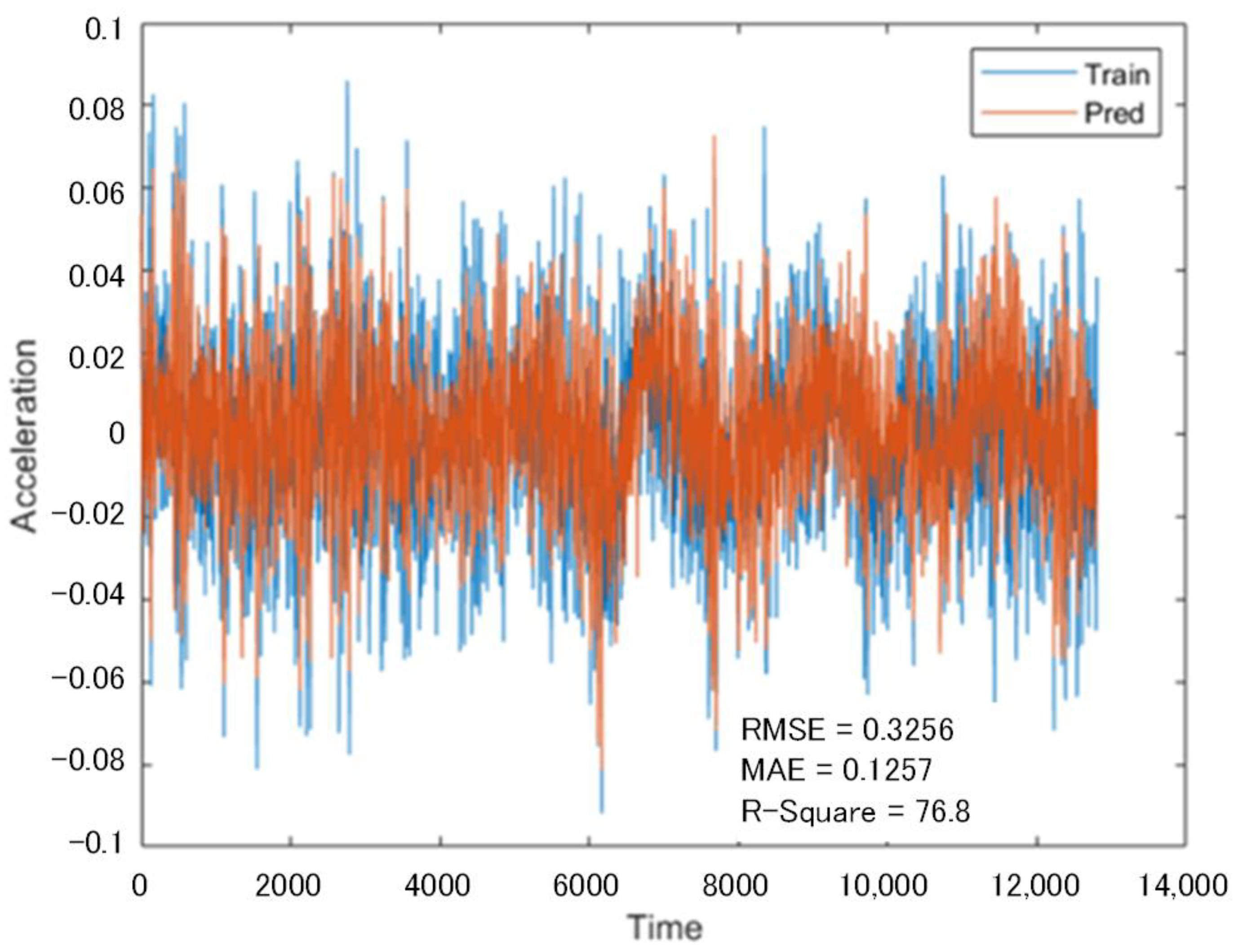
When a subway train passed, a set of 12.8 s vibration signals were generated, and then the collected eight-channel vibration signals were used as the training network. Channels 1–6 were used as test predictor variables (XTest), and Channels 7–8 were used as the response sequence (YTest). The LSTM network was used to predict the incomplete sequences that lacked data from Channels 7 and 8. The prediction results from the training network are shown in Figure 4 and Figure 5. Figure 4 showcases the prediction of the missing data for Channel 7, while Figure 5 showcases that for Channel 8. It can be observed from the figures that this training network can correctly demonstrate the relationships between the data from Channels 1–6 and those from Channels 7 and 8.

The user-specified parameters in the above neural network are optimized to maintain the model’s training accuracy and speed. The optimization results are as follows:

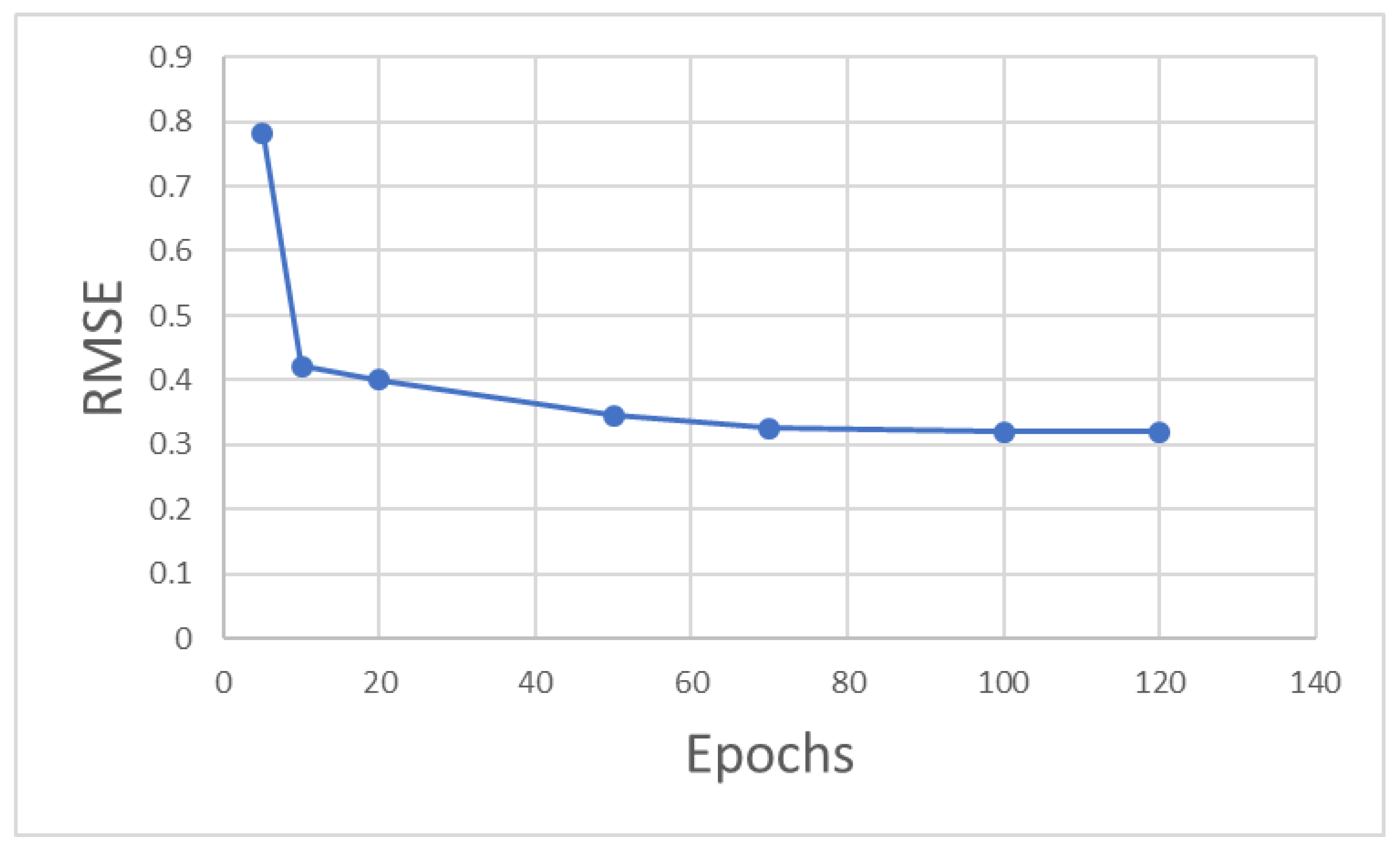
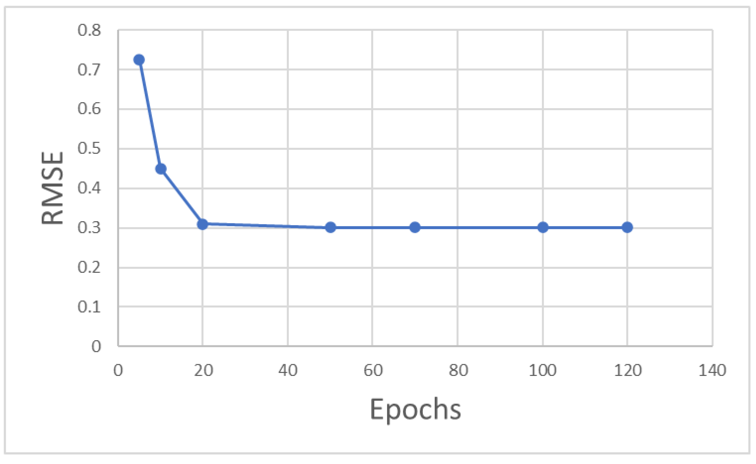
Effect of Epoch on Model Accuracy

As shown in Figure 6, when the epoch value is less than 50, the RMSE value drops rapidly. The decline rate of the RMSE value slows down with the continuous increase in epoch value, and the RMSE region stabilizes when the epoch value exceeds 100. Therefore, 100 is selected as the epoch value for this model by considering the computational accuracy and efficiency.

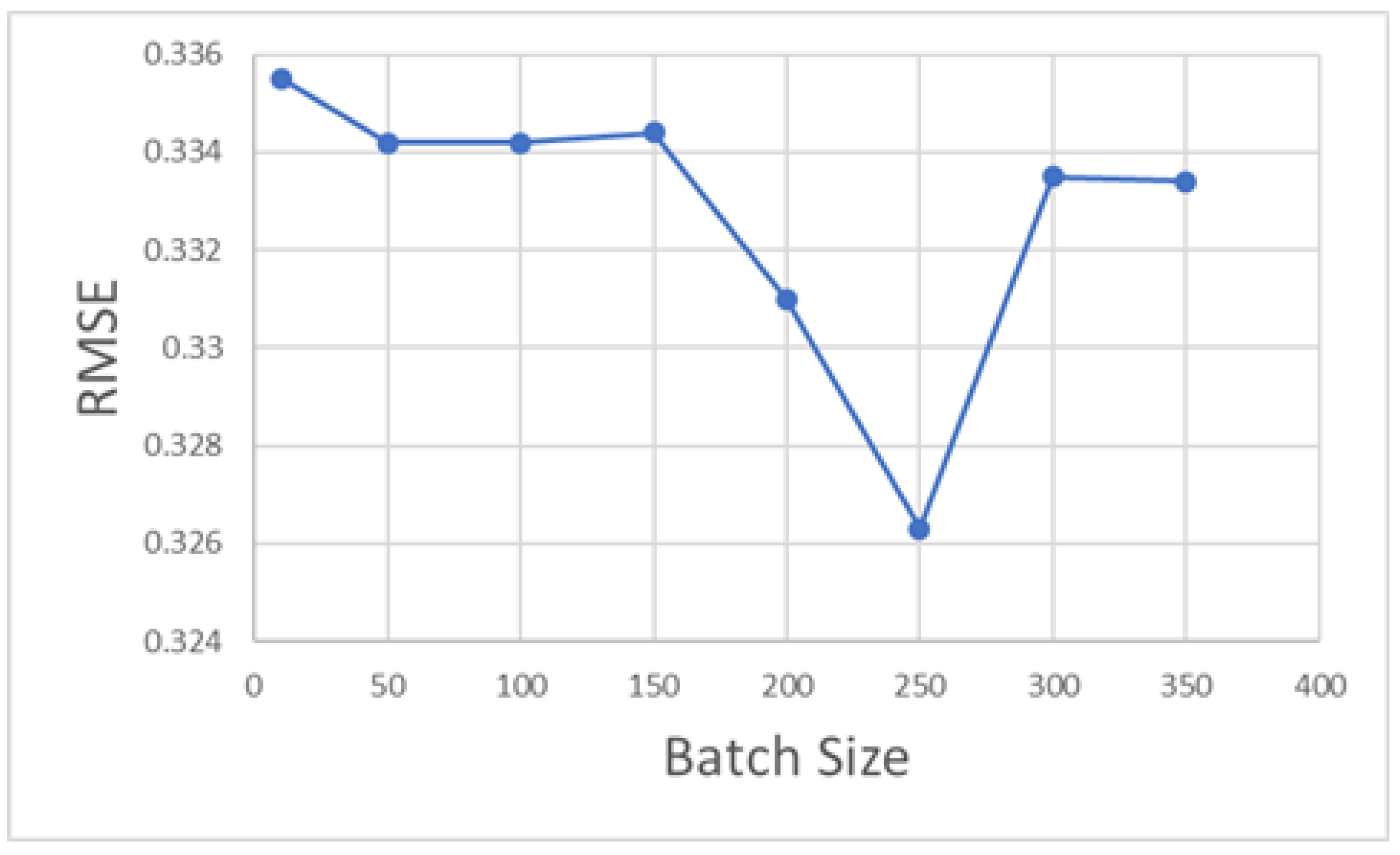
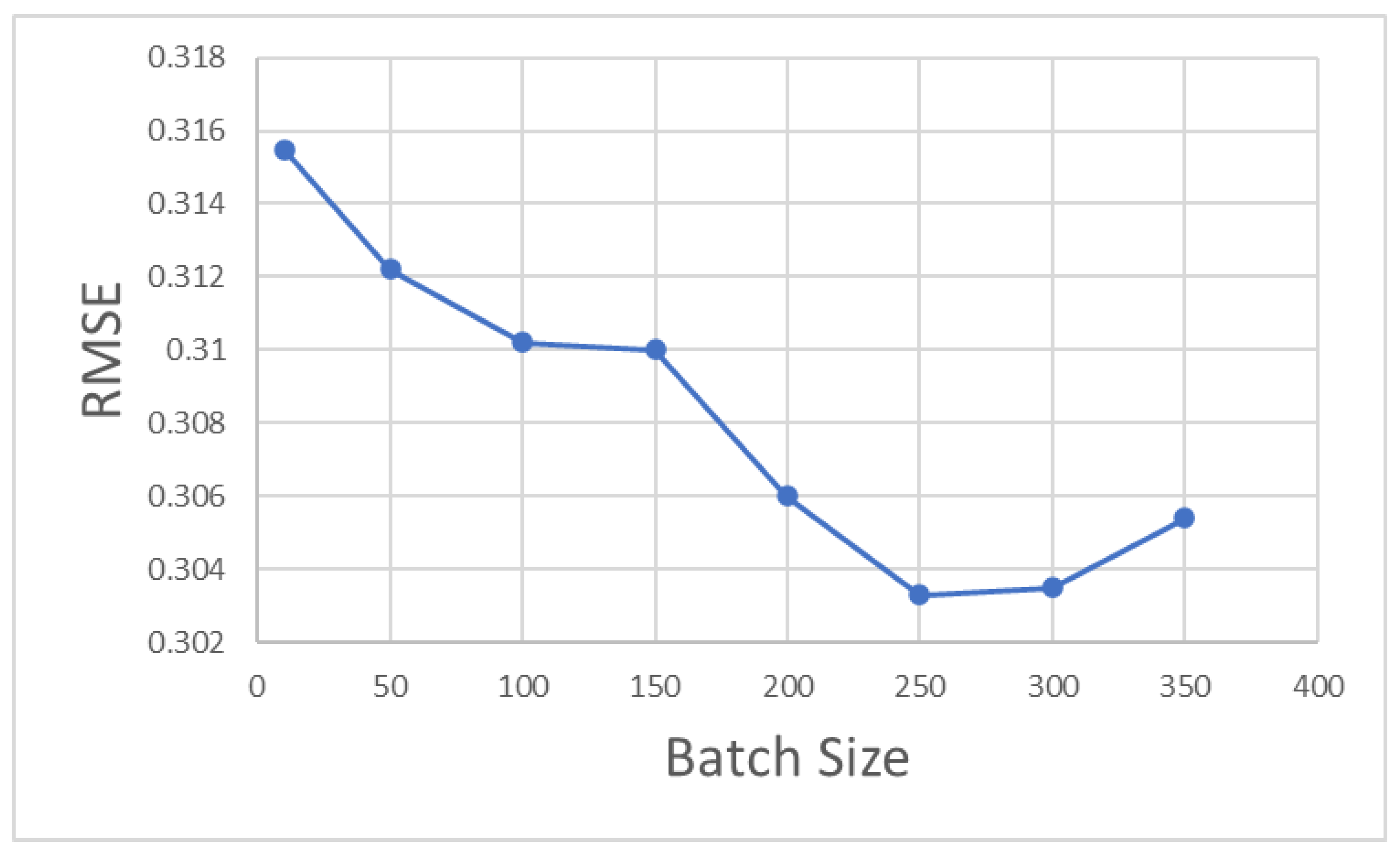
Effect of Batch Size on Model Accuracy

An appropriate batch size selected in an LSTM can increase the model accuracy and reduce the model’s training time. As shown in Figure 7, the value of the RMSE shows a trend of first decreasing and then increasing with the increase in batch size in this model. When the batch size is selected as 250, the value of the RMSE is the minimum, and so 250 is used as the value of the batch size for this model.

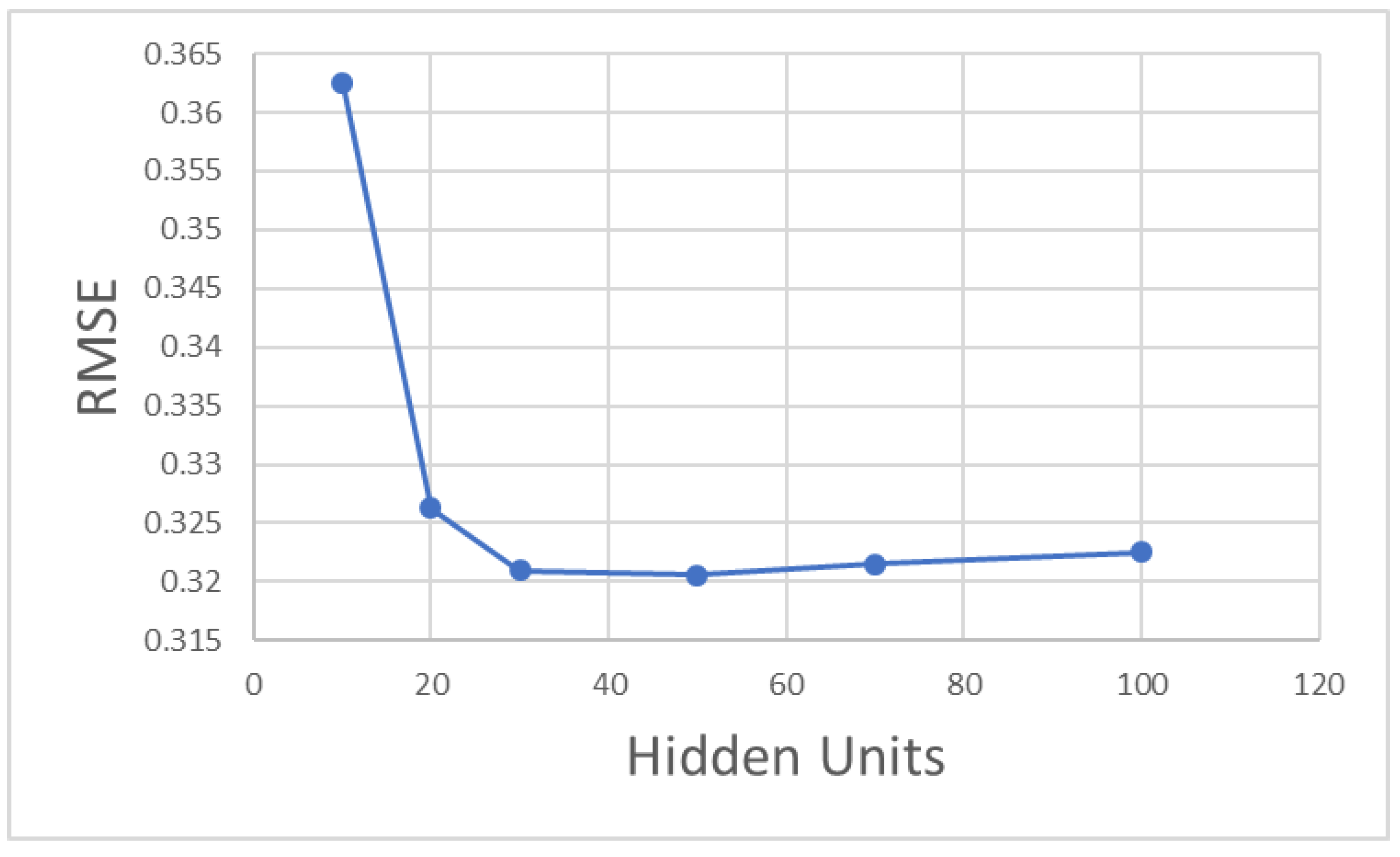
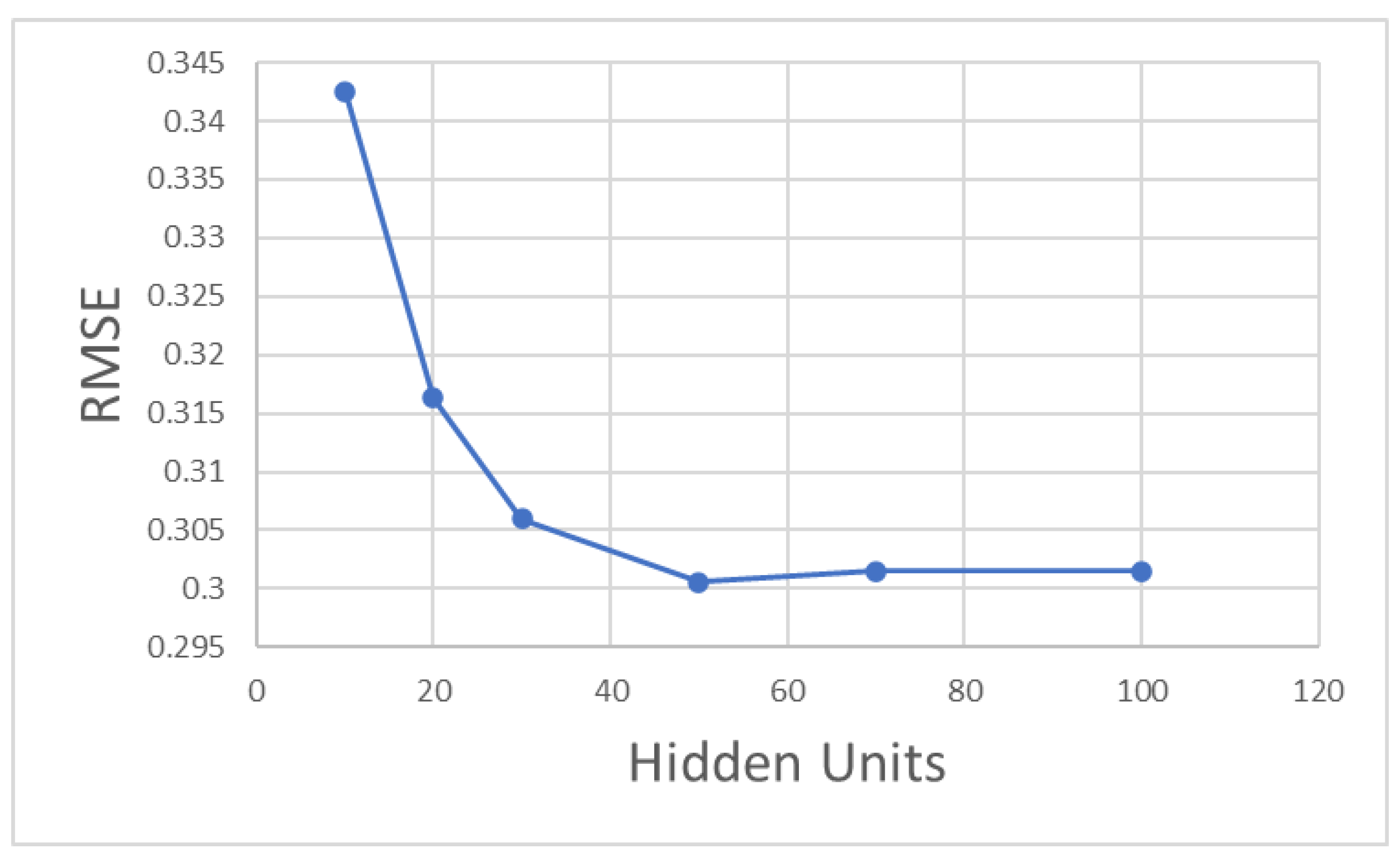
Effect of the Number of Hidden Units in the LSTM Layer on Model Accuracy

When the number of hidden units is less than 30, the RMSE of the training model drops rapidly, as shown in Figure 8. When the number of hidden units is up to 50, the RMSE value is the minimum. As the number of hidden units continues to increase, the RMSE value tends to increase slowly. Therefore, 50 is selected as the value of the number of hidden units in the LSTM layer for this model.

3.1.2. Analysis of Training Results

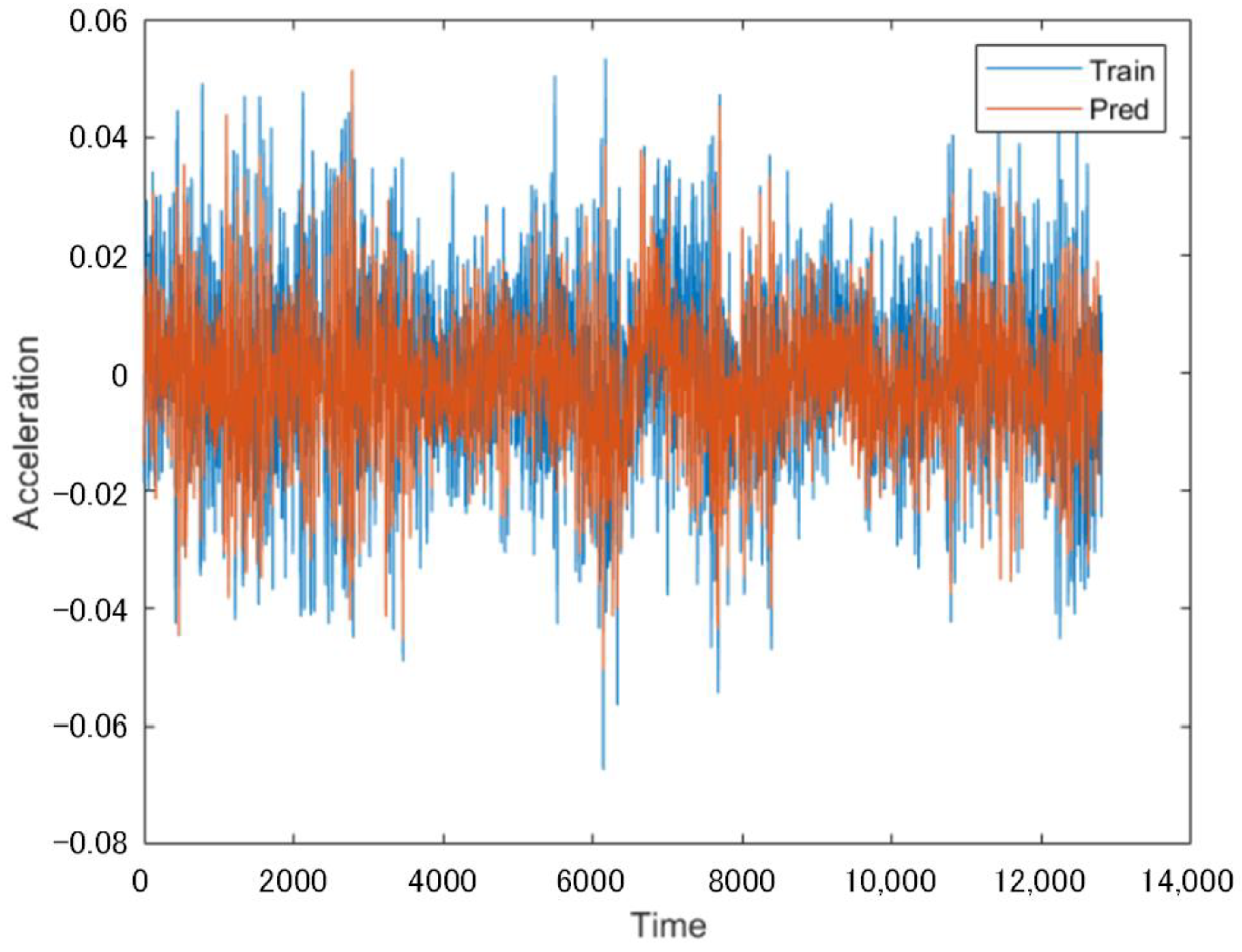
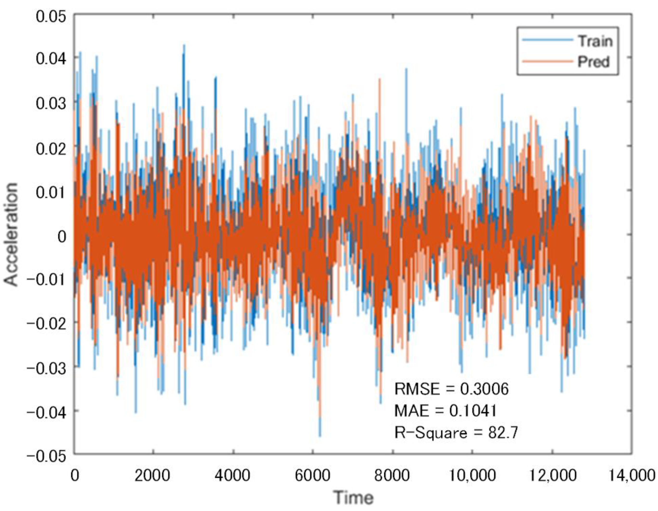
Another set of 12.8 s vibration signals collected from the same subway at the same location but at different times was used as a test network, and the LSTM network as trained above was used to predict the incomplete sequences that lacked data from Channels 7 and 8. Figure 9 indicates the prediction of the lost data in Channel 7, and Figure 10 represents the prediction of the lost data in Channel 8. As shown in the above figures, the vibration signal predicted by the multi-channel data recovery model proposed in this paper based on the lost data recovery model of adjacent channel time series is largely consistent with the real vibration signal curve.

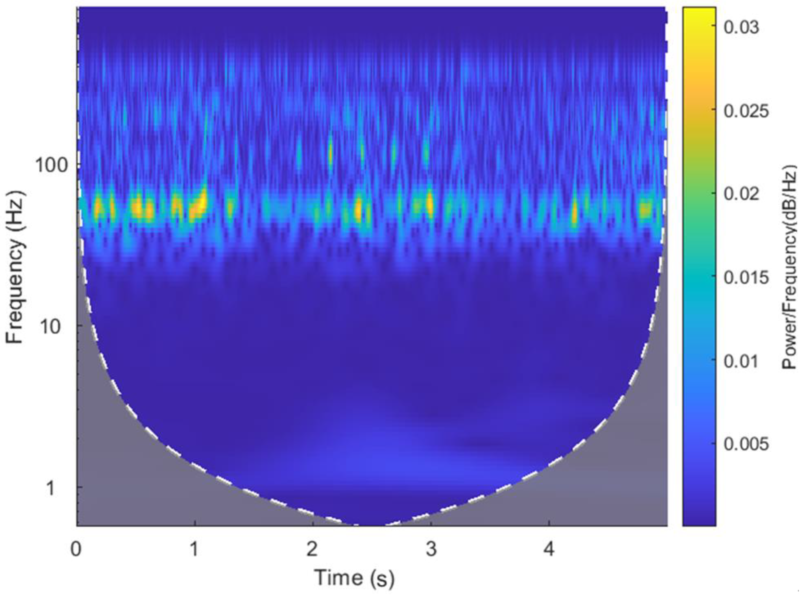
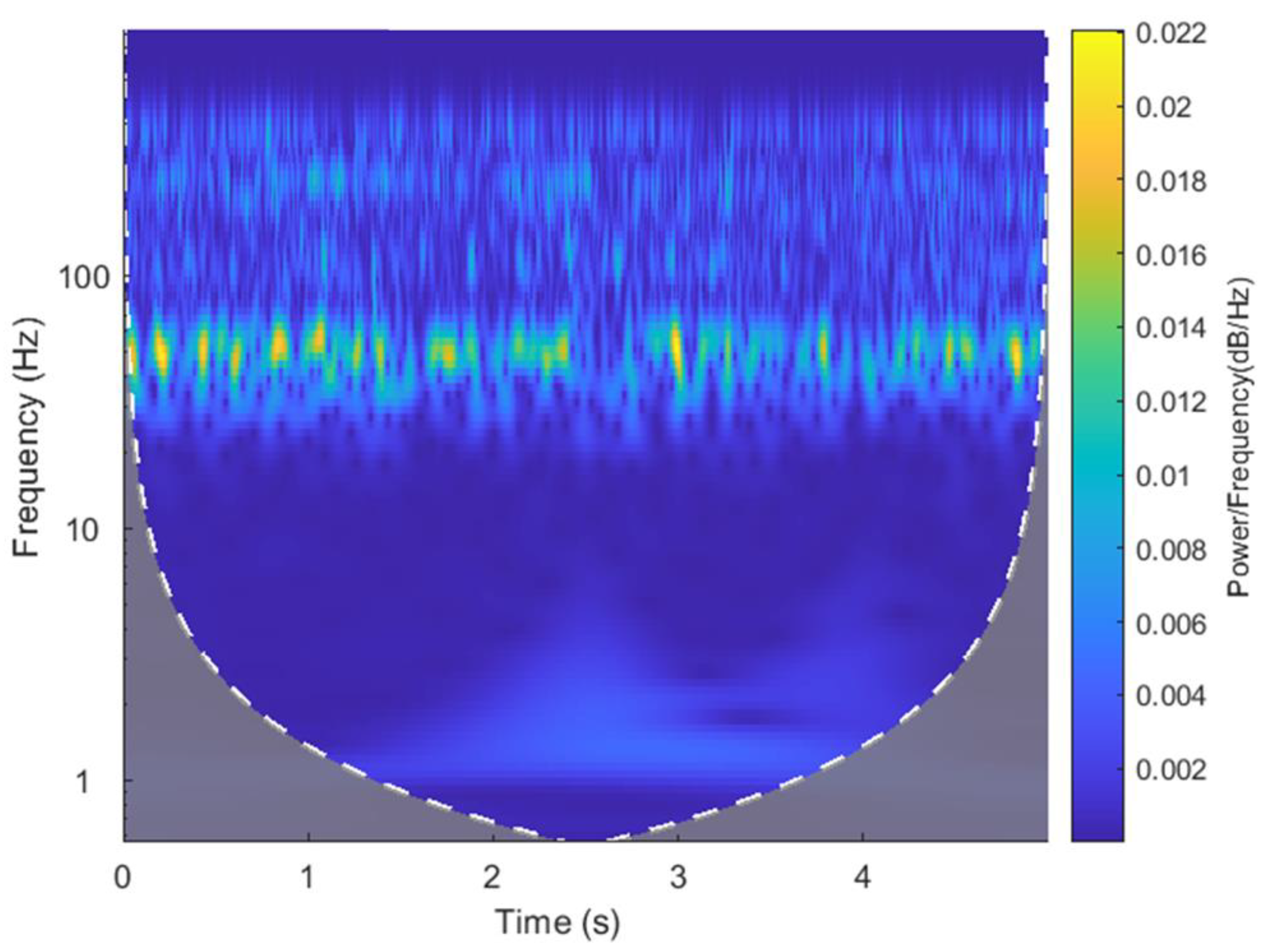
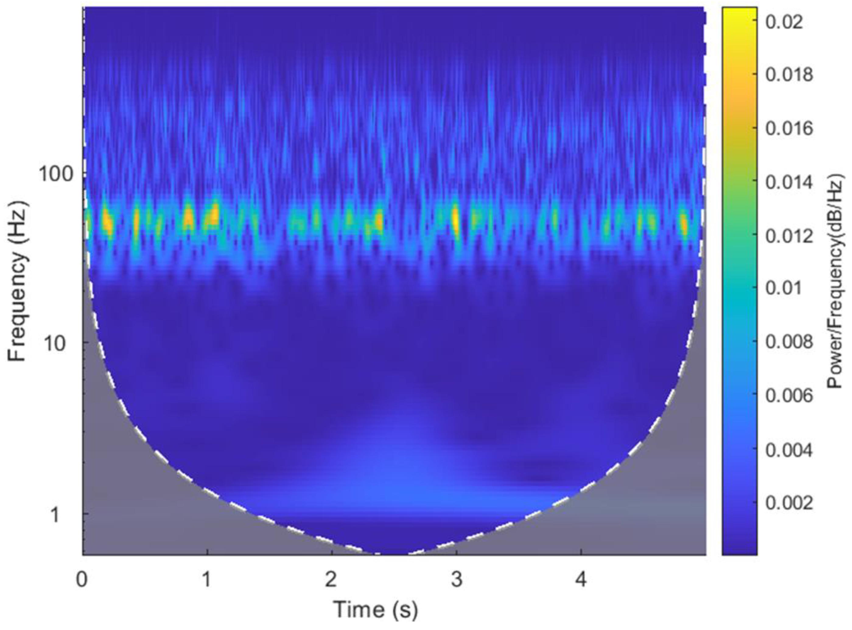
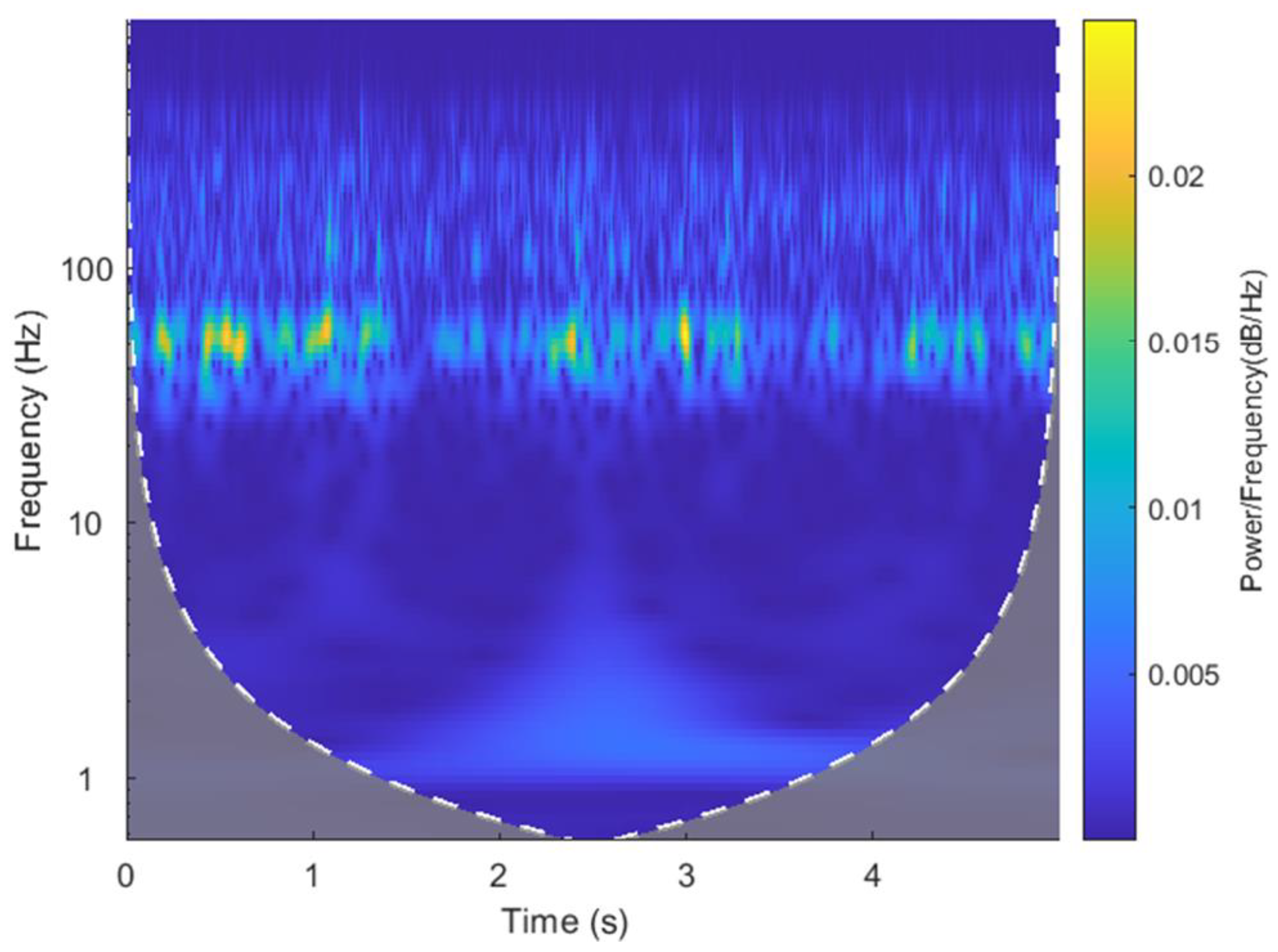
The vibration acceleration signal is further wavelet-transformed to obtain a more intuitive time-frequency image of Channel 7’s vibration acceleration frequency over time. Figure 11 shows the wavelet-transformed time-frequency image of the measured value, and Figure 12 shows the wavelet-transformed time-frequency image of the predicted value. It can be seen from the figures that the change trend in signal frequency of the missing data’s predicted value and measured value over time is largely the same, and that the peak frequency appears at approximately the same position.

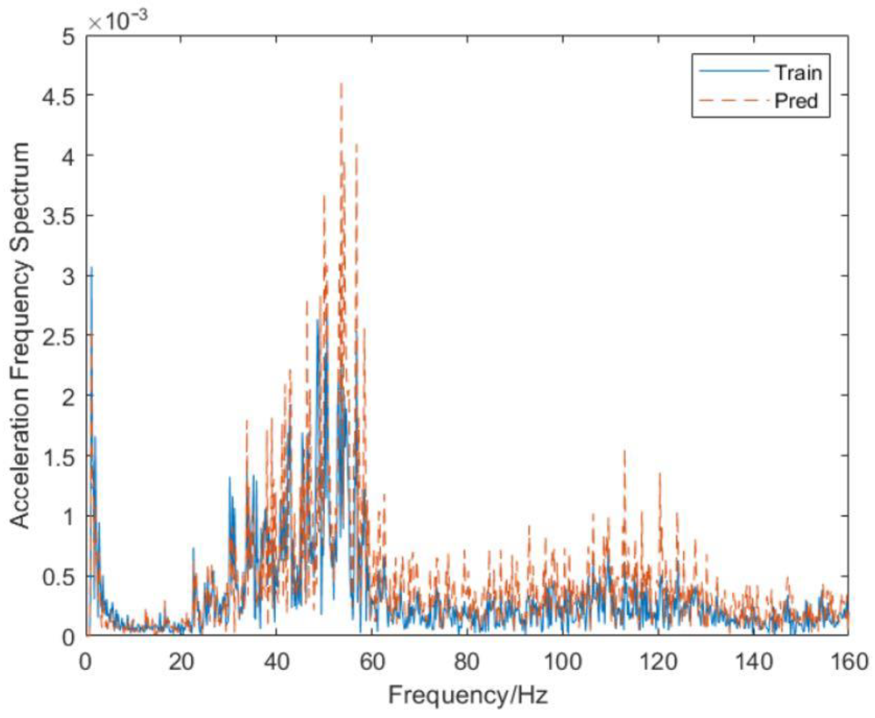
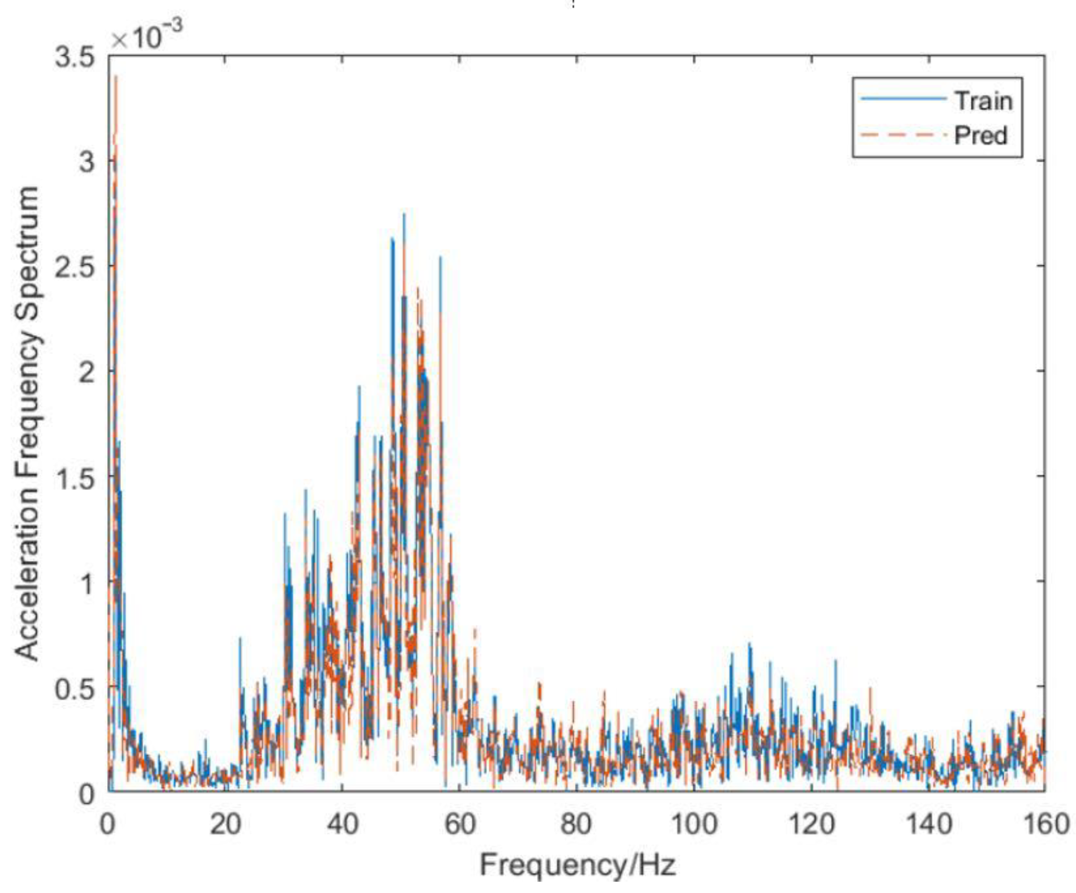
A Fourier transform is performed on the vibration acceleration signal to obtain a more intuitive comparison diagram of the vibration acceleration amplitude loss data prediction and actual measurement of Channel 7, as shown in Figure 13, and the predicted value of the lost data is consistent with the actual value at all frequencies.

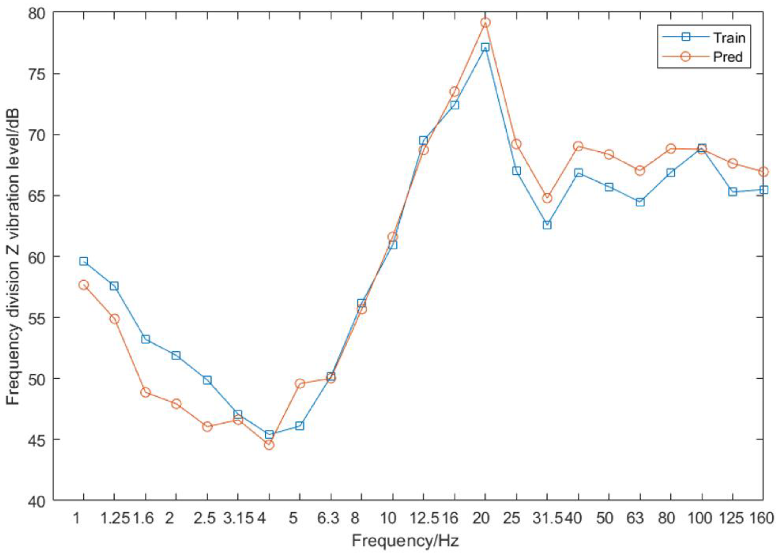
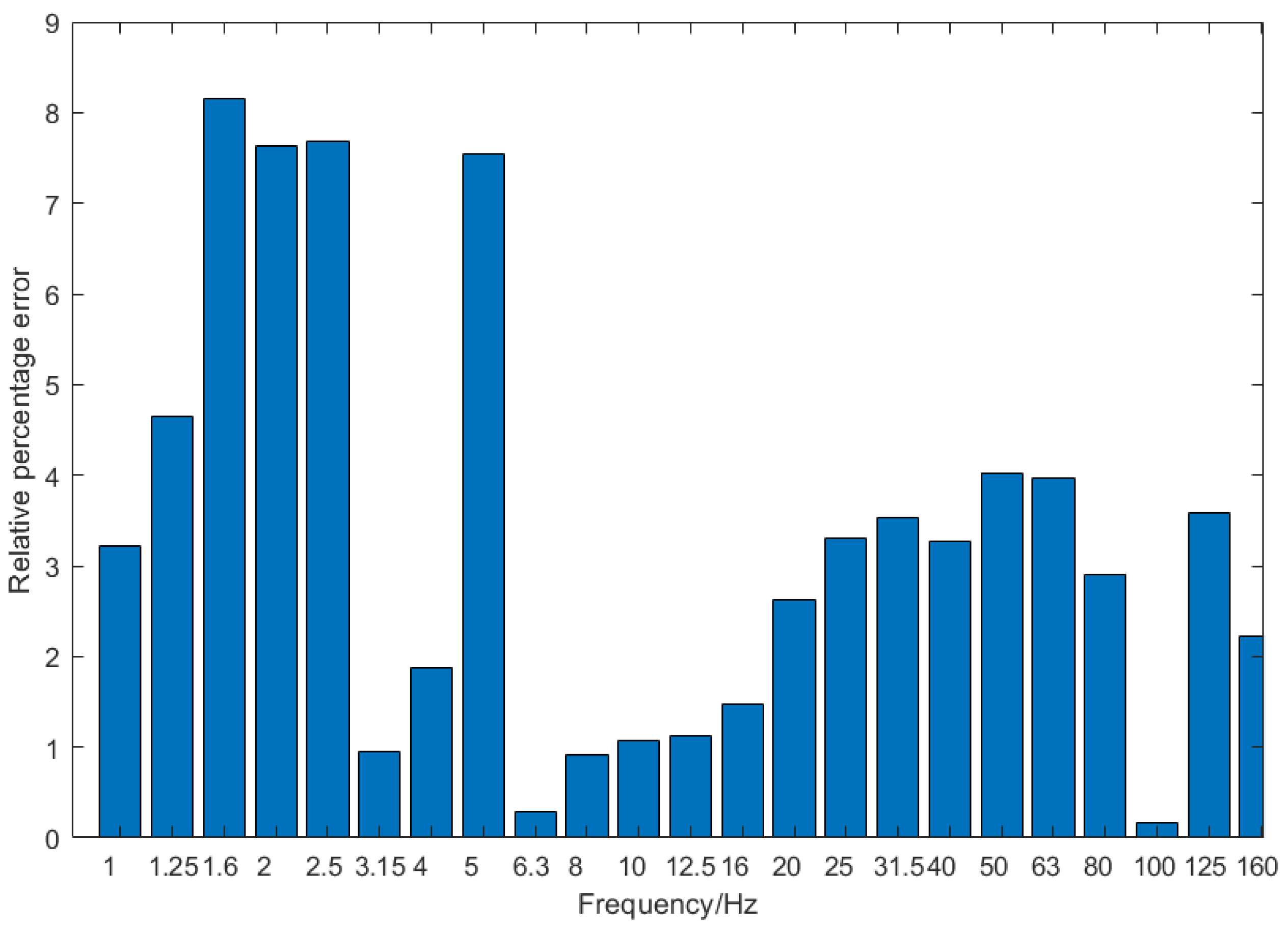
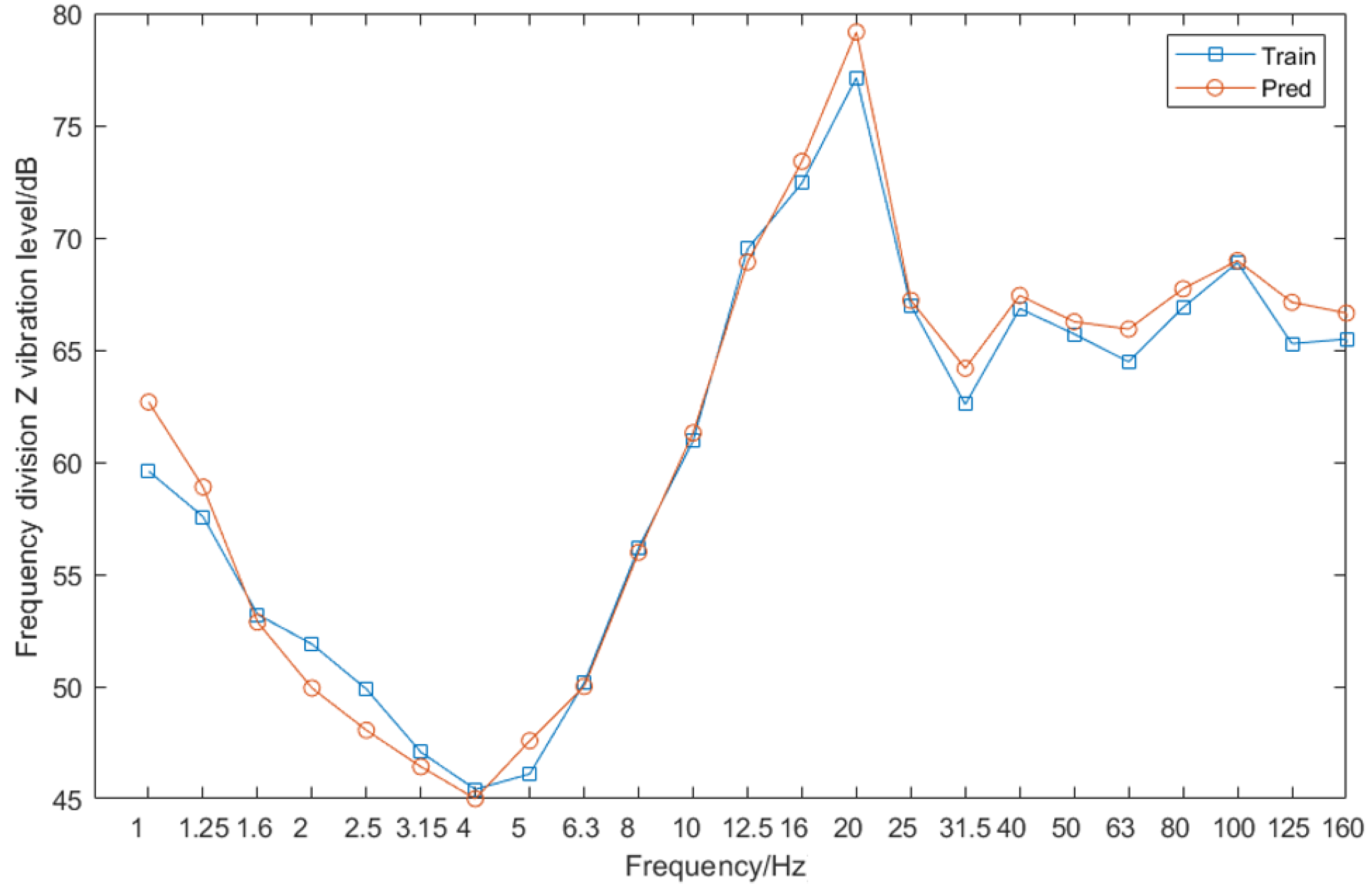
Figure 14 shows the comparison between the predicted data of the LSTM neural network and the actual vibration acceleration data at different frequencies. It can be seen that the predicted data and the actual data have the same trend at all frequencies. Since Channel 7 is from the sensor on the tunnel wall, the accuracy of the predicted data between 10 and 100 Hz is mainly analyzed. The relative error between the predicted data and the actual data is calculated, as shown in Figure 15, and the error values at all frequencies are less than 10%, the overall accuracy rate is up to 95%, and for the 10–100 Hz frequency of interest, the accuracy rate reaches 97%.

3.2. Training the Network by Using Frequency-Domain Data

3.2.1. Training Process of the Neural Network

By using the same set of 12.8 s vibration signals in Section 3.1.1, a Fourier transform was performed on the Channel 8 data. After the transform, Channels 1–6 were used as the test predictor variables (XTest2) and Channels 7–8 as the response sequence (YTest2), while keeping the other parameters consistent with those in Section 3.1.1, and the LSTM network was used to predict the incomplete sequence that lacked data from Channels 7 and 8. The prediction results from the training network for the missing data from Channel 7 are shown in Figure 16.

The user-specified parameters in the above neural network are optimized to maintain the model’s training accuracy and speed. The optimization results are as follows:

Effect of Epoch on Model Accuracy

As shown in Figure 17, when the epoch value is less than 20, the RMSE value drops rapidly. The decline rate of the RMSE value slows down with the continuous increase in epoch value, and the RMSE region stabilizes when the epoch value exceeds 50. Therefore, 50 is selected as the epoch value for this model by considering the computational accuracy and efficiency.

Effect of Batch Size on Model Accuracy

An appropriate batch size selected in an LSTM can increase the model’s accuracy and reduce the model’s training time. As shown in Figure 18, the value of the RMSE shows a trend of first decreasing and then increasing with the increase in batch size in this model. When the batch size is selected as 250, the value of the RMSE is the minimum, and so 250 is used as the value of the batch size for this model.

Effect of the Number of Hidden Units in the LSTM Layer on Model Accuracy

When the number of hidden units is less than 30, the RMSE of the training model drops rapidly, as shown in Figure 19. When the number of hidden units is up to 50, the RMSE value is the minimum. As the number of hidden units continues to increase, the RMSE value tends to increase slowly. Therefore, 50 is selected as the value of the number of hidden units in the LSTM layer for this model.

In general, the model built with frequency-domain data achieves faster iterative efficiency in the training process than that built with time-domain data. The overall time spent on training is shorter, with lower losses and RMSE, MEA, and R2 values.

3.2.2. Analysis of Training Results

By using another set of 12.8 s vibration signals in Section 3.1.2 at the same location, a Fourier transform was performed on the vibration signals. The LSTM network as trained above was used to predict the incomplete sequences that lacked data from Channels 7 and 8, with the prediction results shown in Figure 20. Compared with prediction using raw time domain data, where a Fourier transform was performed after the original data were used to make a prediction, Figure 20 shows that the predicted signal curves fit more closely to the vibration curves.

After the inverse Fourier transform, the vibration acceleration signal is further wavelet-transformed to obtain a more intuitive time-frequency image of Channel 7’s vibration acceleration frequency over time. Figure 21 shows the wavelet-transformed time-frequency image of the measured value, and Figure 22 shows the wavelet-transformed time-frequency image of the predicted value. It can be seen from the figures that the height of the signal frequency of the missing data’s predicted value and measured value over time is approximately the same, and that the peak frequency appears at approximately the same height.

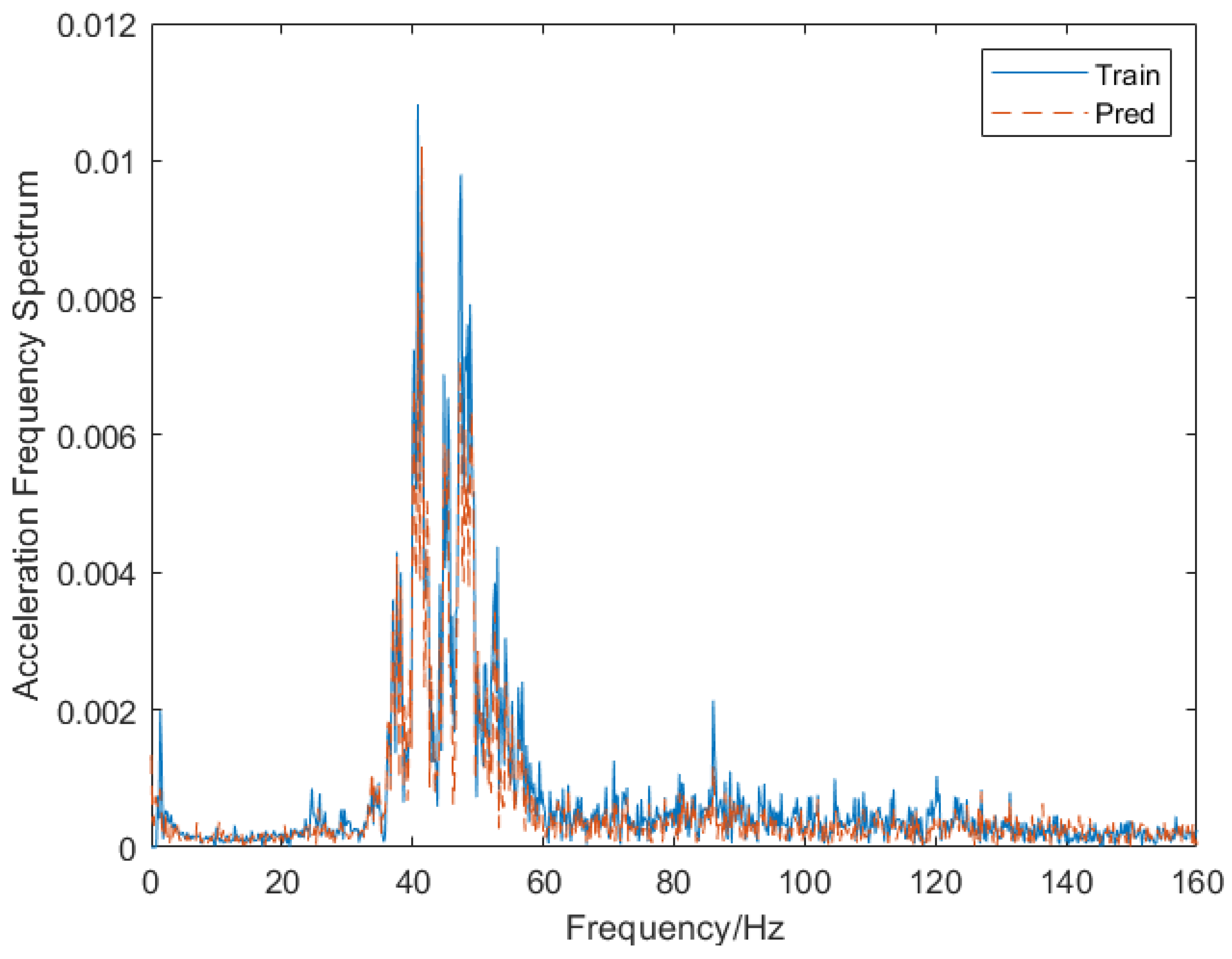
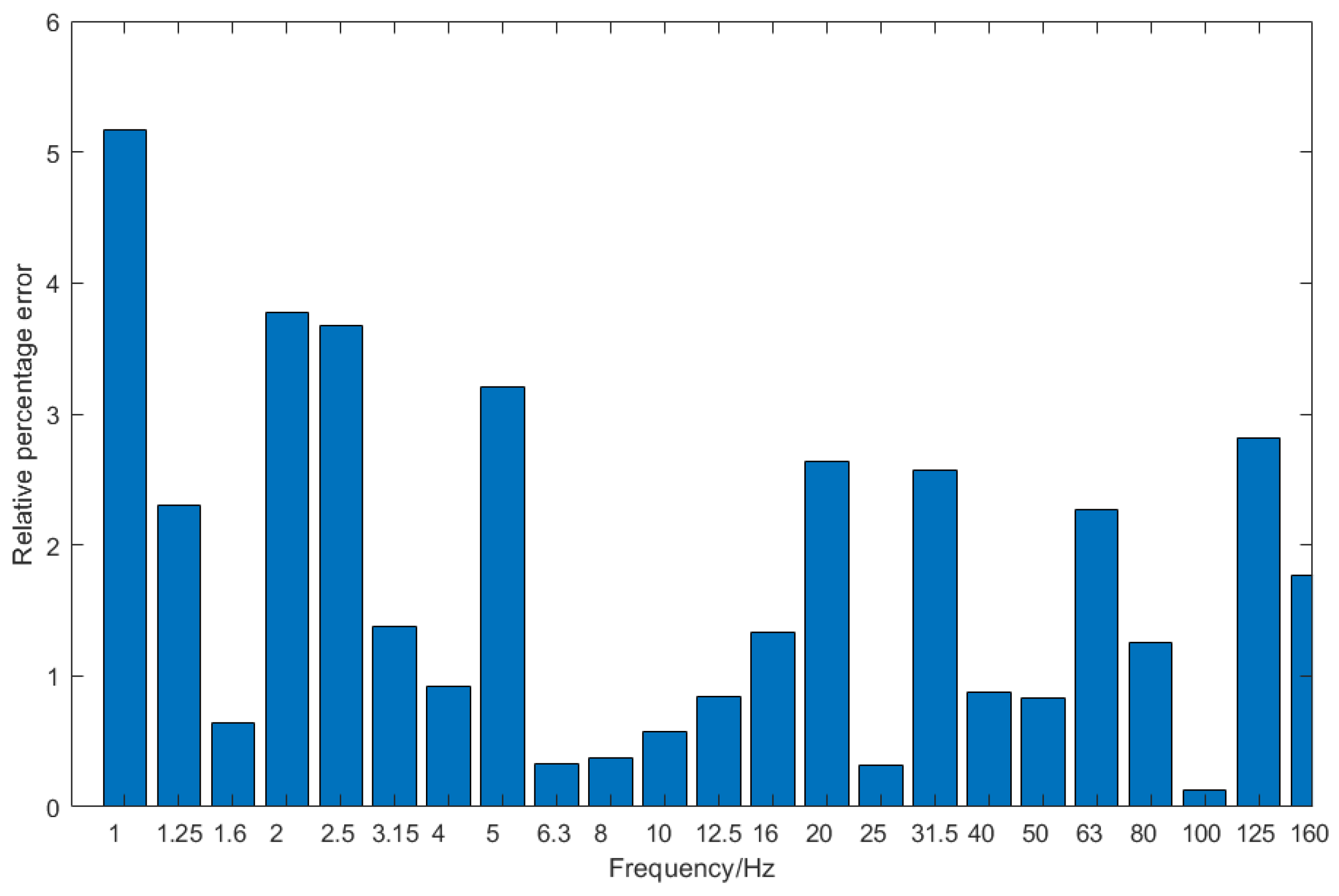
After an inverse Fourier transform was further performed on the predicted frequency-domain data, the corresponding time-domain data could be obtained, as shown in Figure 23. Then, the vibration acceleration data acquired were processed in the one-third octave. Figure 24 shows the one-third octave center frequency spectrum of Channel 7’s vibration acceleration value as predicted with the Fourier transform data, as well as that spectrum of Channel 7’s real value. Figure 25 shows the percentage difference between actual and predicted values. Figure 25 demonstrates smaller errors at all frequencies than those shown in Figure 15, especially between 1 and 10 Hz. The overall accuracy rates of as high as 98% indicate that the method can deliver higher accuracy rates.

In summary, in the scenarios of collecting multi-channel data, this model can use the data from adjacent channels to restore the data of the lost channels and ensure that the restored data have high accuracy. This method can reduce the cases of discarding whole data groups due to the loss of individual channels’ data. Primarily, if the original data are applied to the LSTM network after performing a Fourier transform, the model can deliver higher accuracy because the processed data have higher correlations than the original data.

4. Conclusions

This study proposes a time-series recovery method using adjacent multi-channel data based on an LSTM neural network. In the case of collecting multi-channel data, the adjacent channel data is used to recover the lost time-series data. Based on the measured data of a subway, a multi-channel data recovery model is established, and the accuracy of the training data is guaranteed by optimizing the parameters of the neural network. This study uses time-domain and frequency-domain data to train the LSTM neural network. The results show that the network trained with time-domain data is 95% accurate for time-series data recovery, while the network trained with frequency-domain data is as high as 98% accurate. Time-domain data can better reflect the internal relationship between adjacent channels so that the trained neural network has higher accuracy. This data recovery method is generally feasible and provides a reference value for further exploration of multi-channel time-series data recovery using machine learning. Currently, this method’s internal connection of multi-channel vibration signals is data-driven. Therefore, it is necessary to further study the internal relationship of data among channels and optimize the model’s algorithm by adding physical information to the neural network. On this basis, weak mechanism modeling theory is used to derive the laws and summarize weak mechanisms. There are two ways to obtain weak mechanisms: first, they can be obtained through derivation from a stronger mechanism, which may be more useful than mathematical analysis, and second, they can be obtained through summarization of the data mainly by means of statistics and machine learning. Then, some weak mechanisms are obtained. Next, proceeding from one or more weak mechanisms, a computable model can be established through a specific combination/fusion, which helps to understand the inherent connection of the data learned by the neural network and further expands the interpretability of the neural network.