
Characterisation of Coastal Sediment Properties from Spectral Reflectance Data


Abstract
:1. Introduction
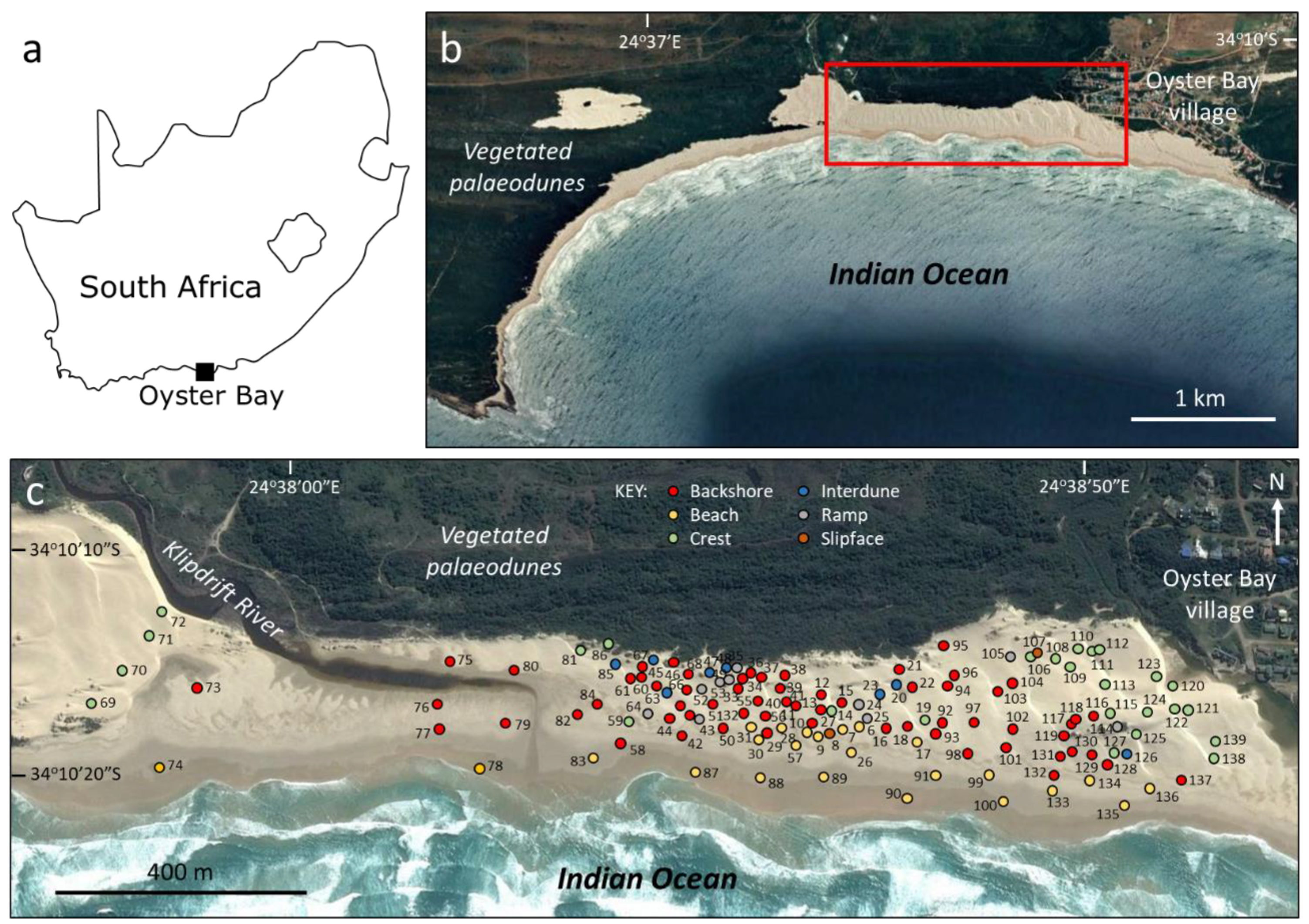
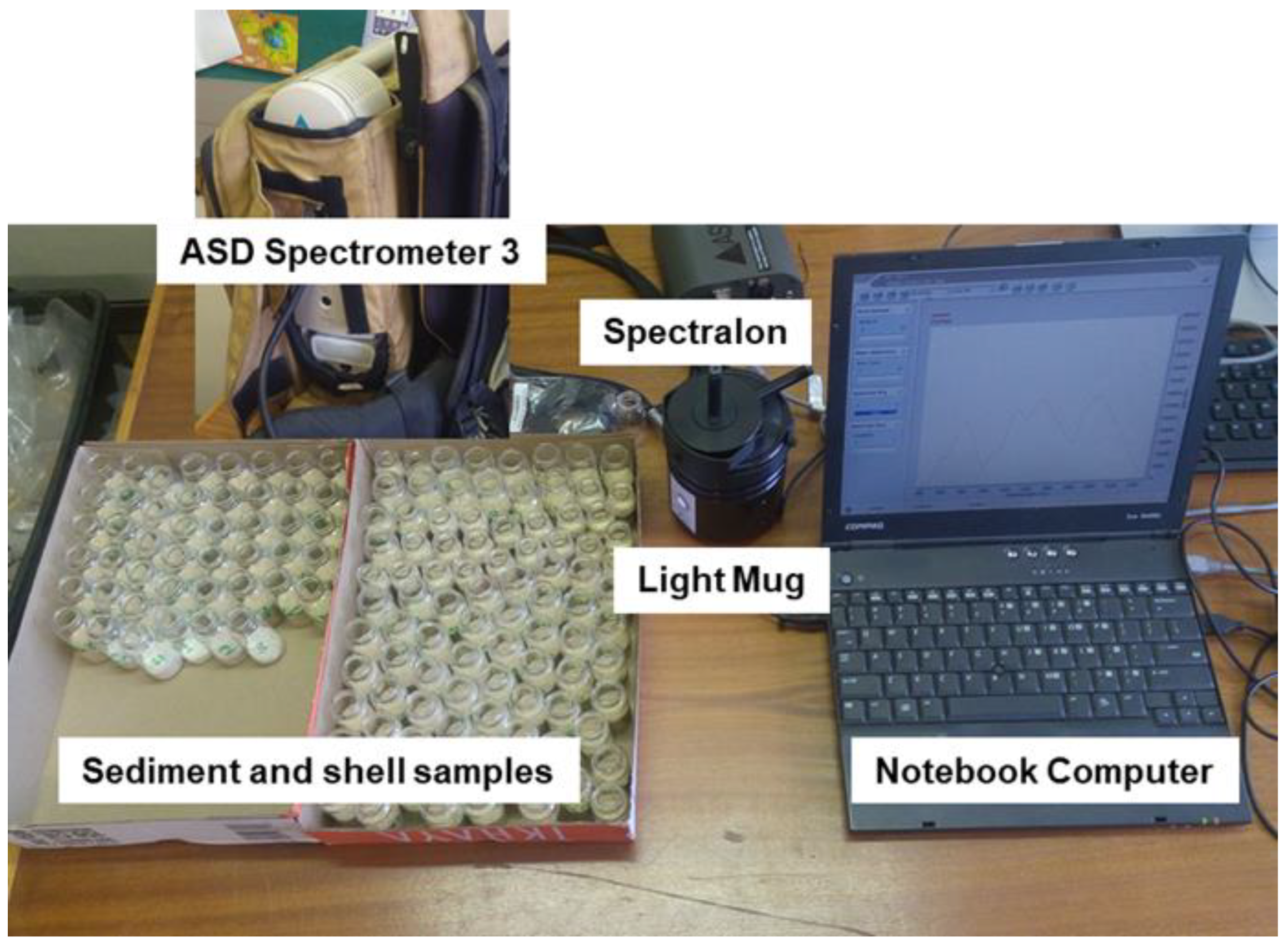
2. Study Area and Methods
3. Results
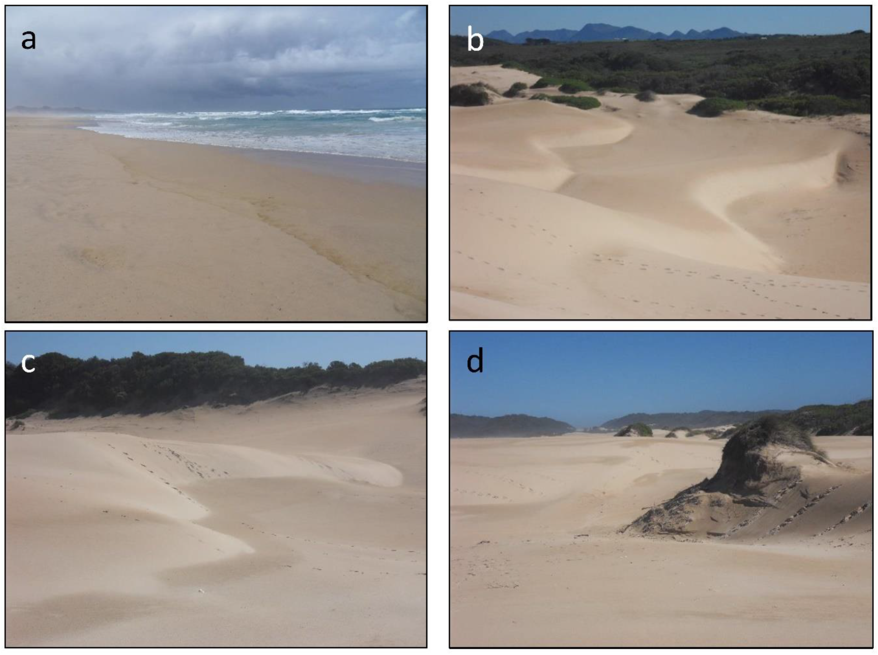
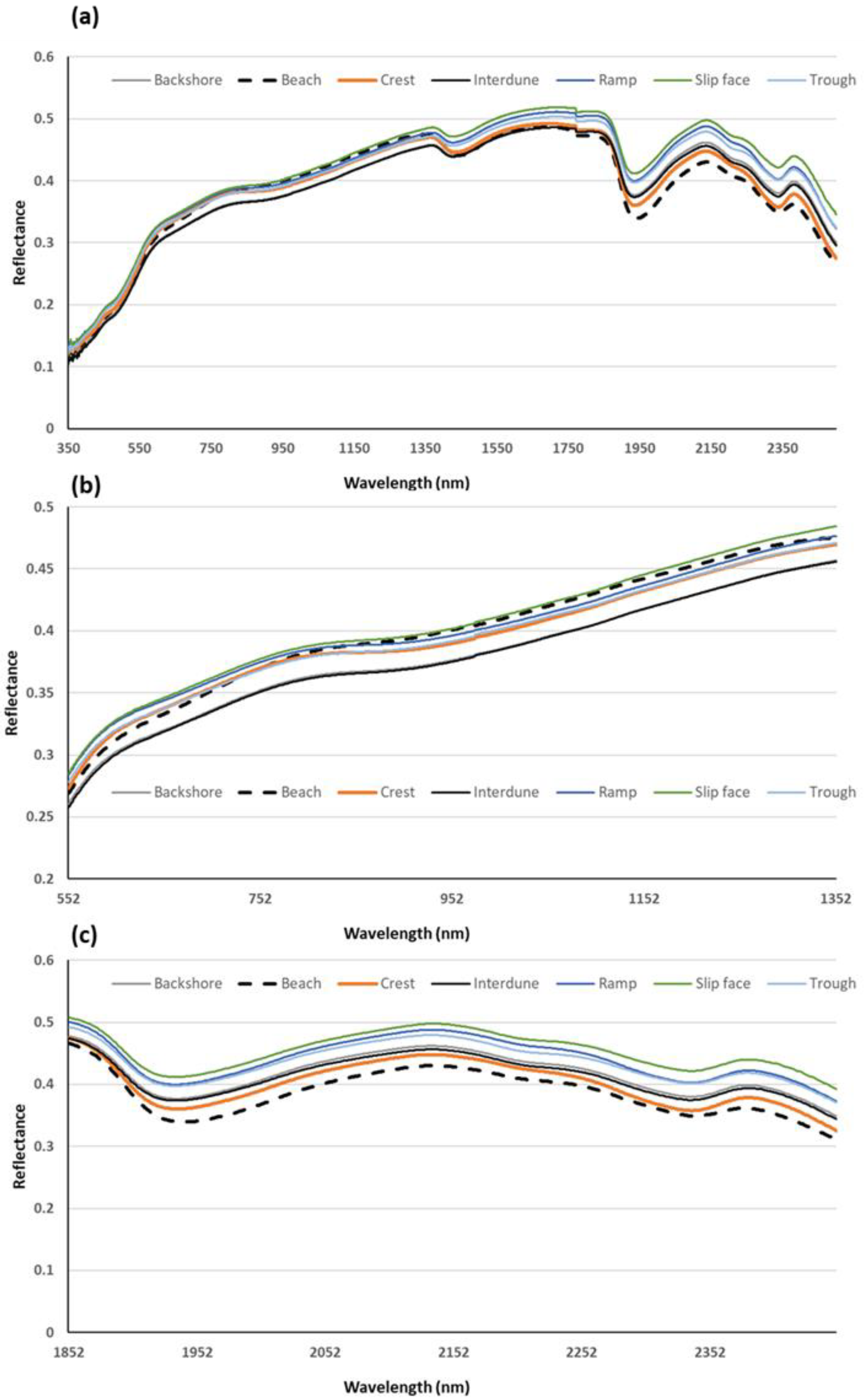
3.1. Site Geomorphology and Sediment Dynamics
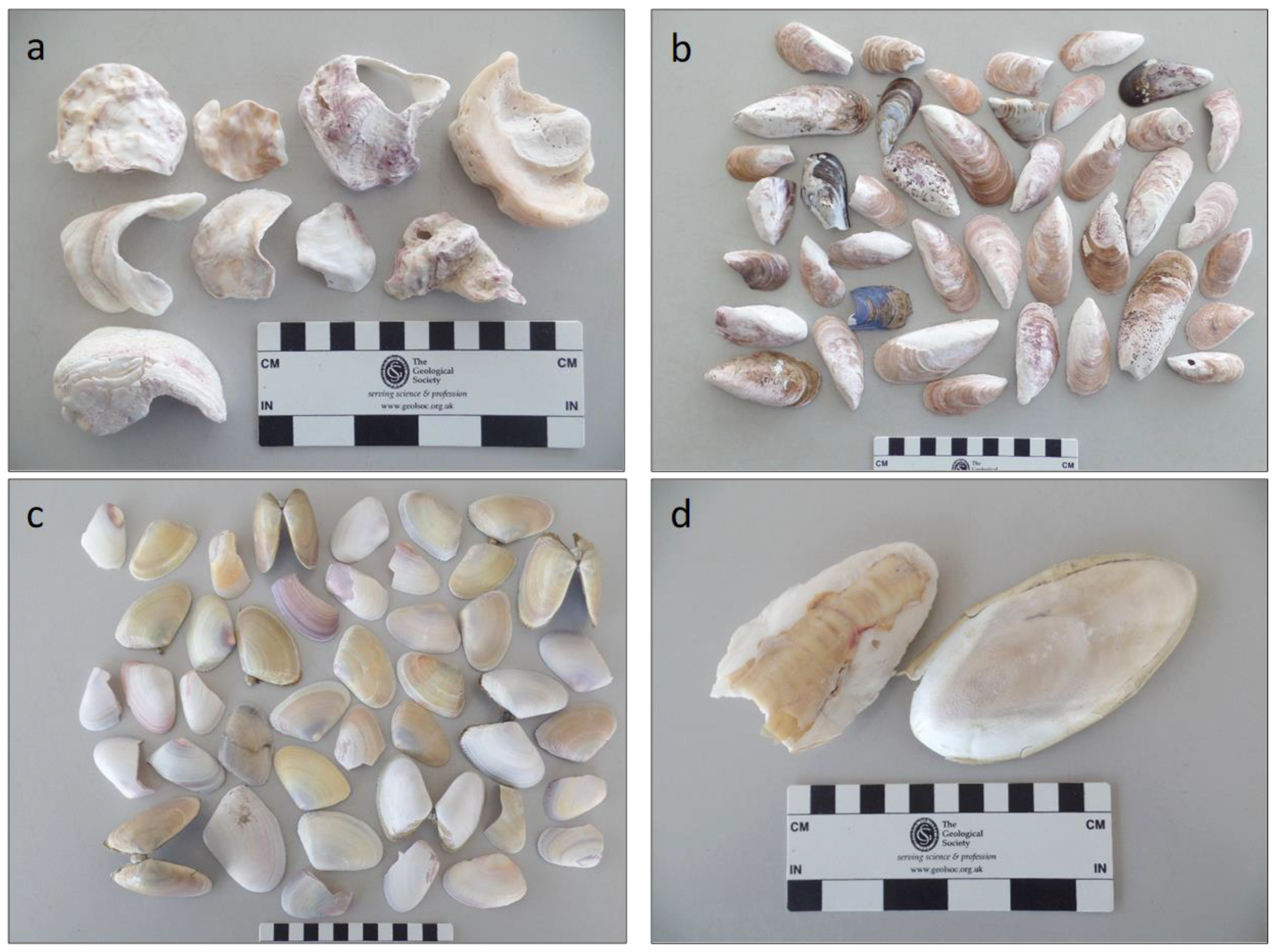
3.2. Sediment Properties
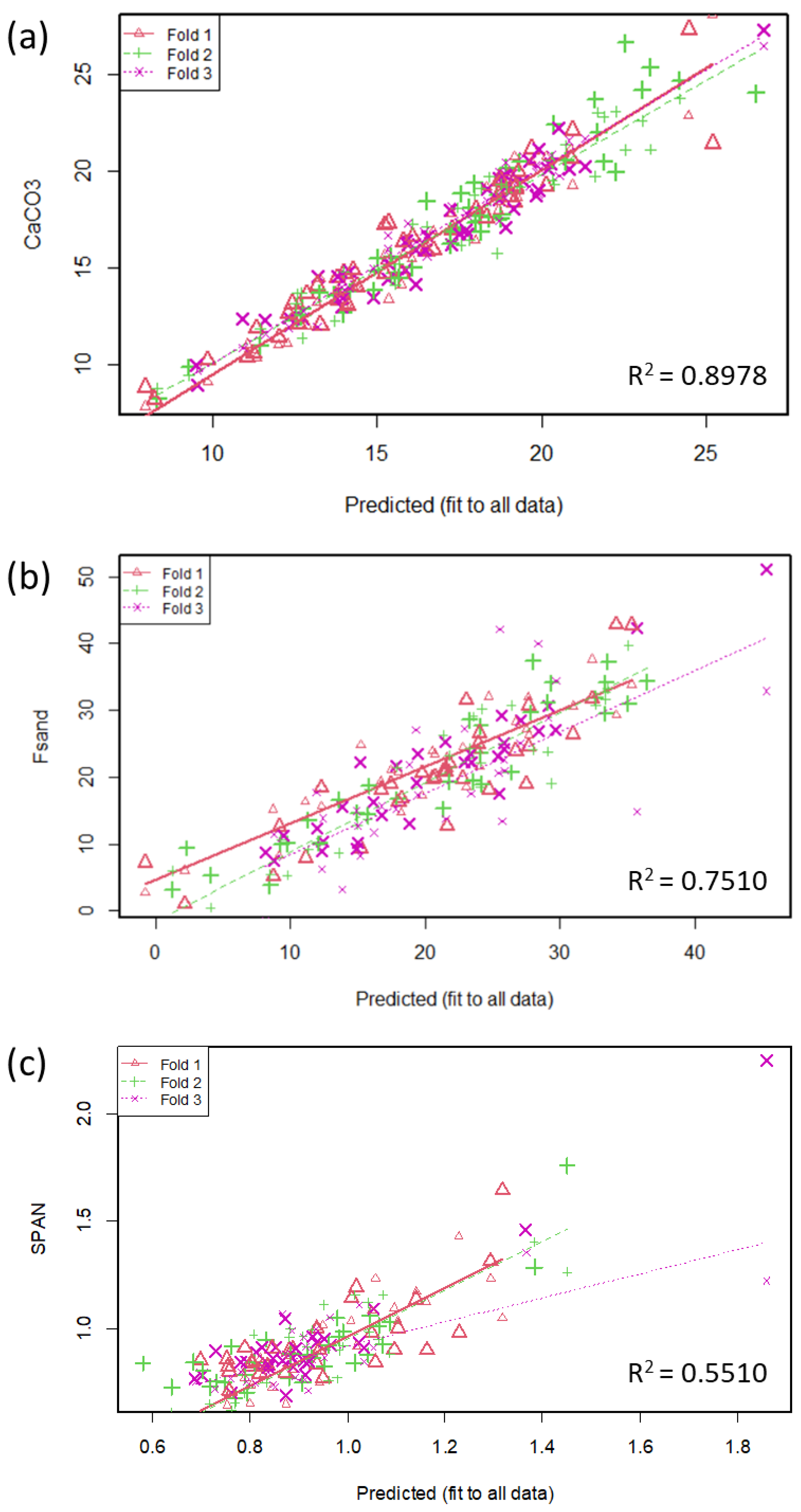
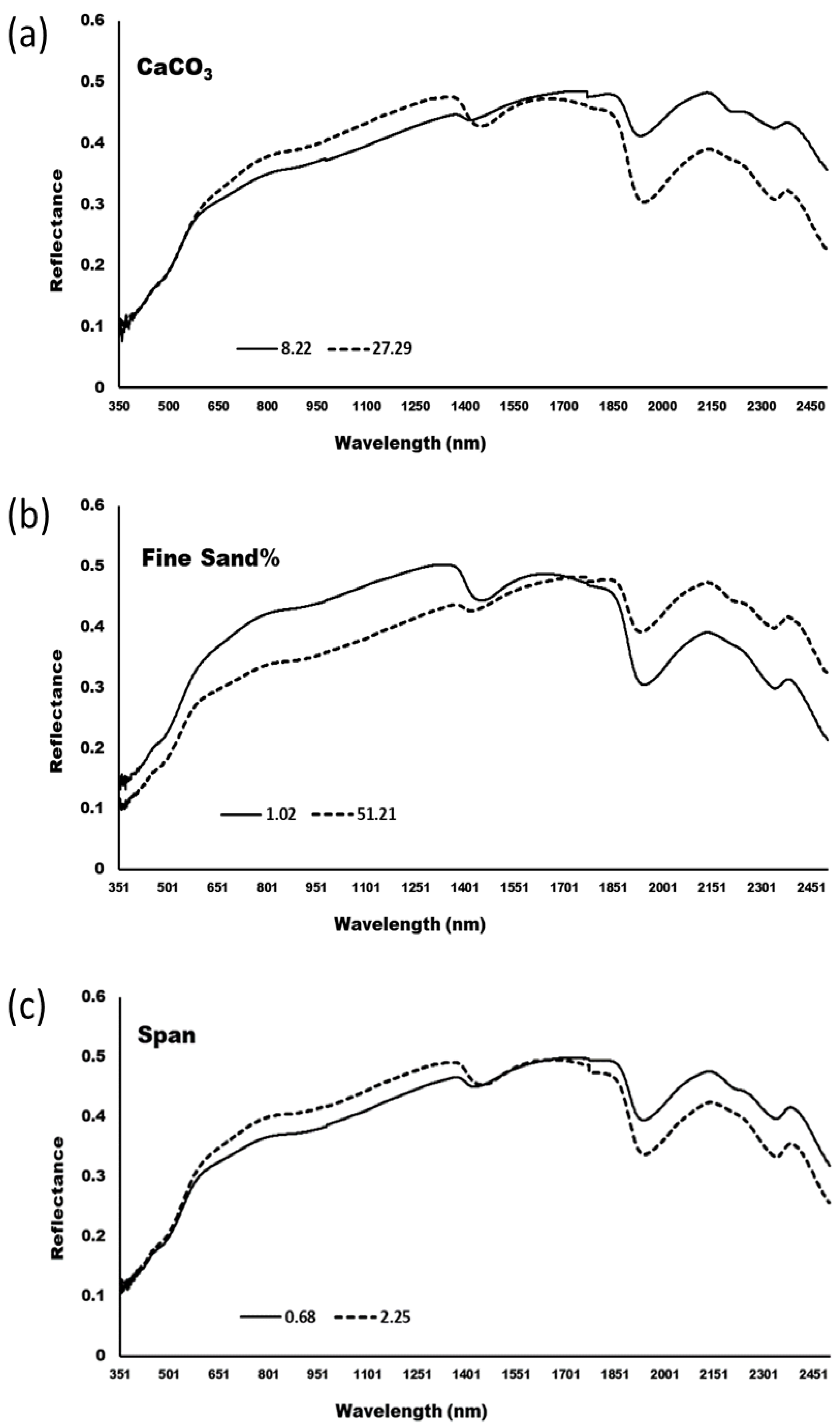
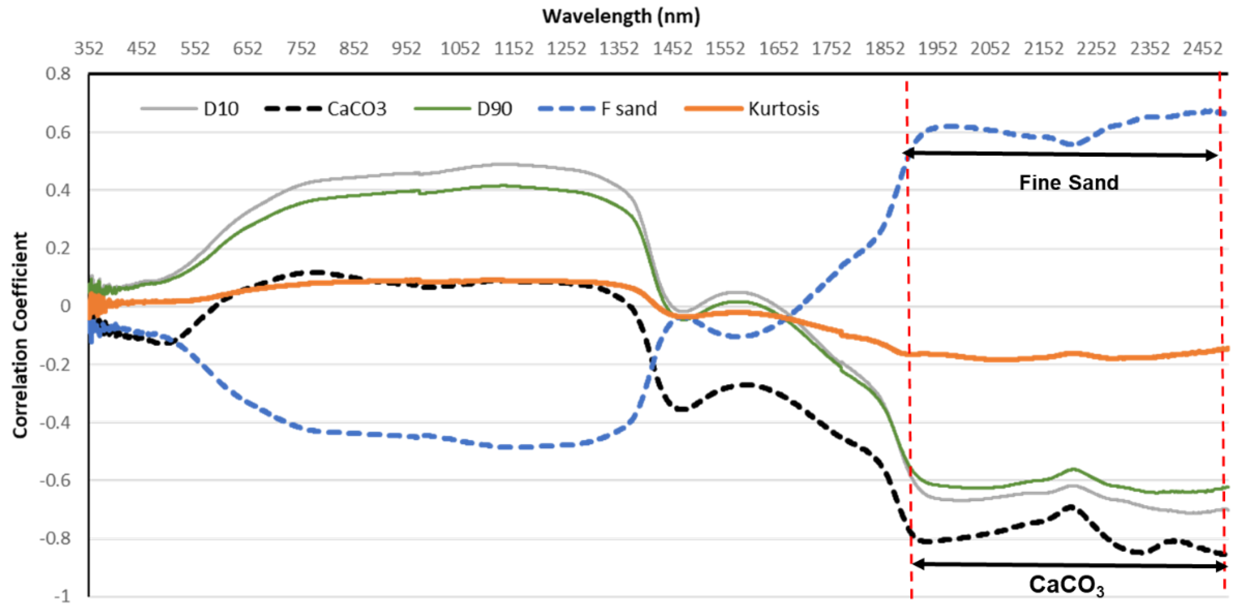
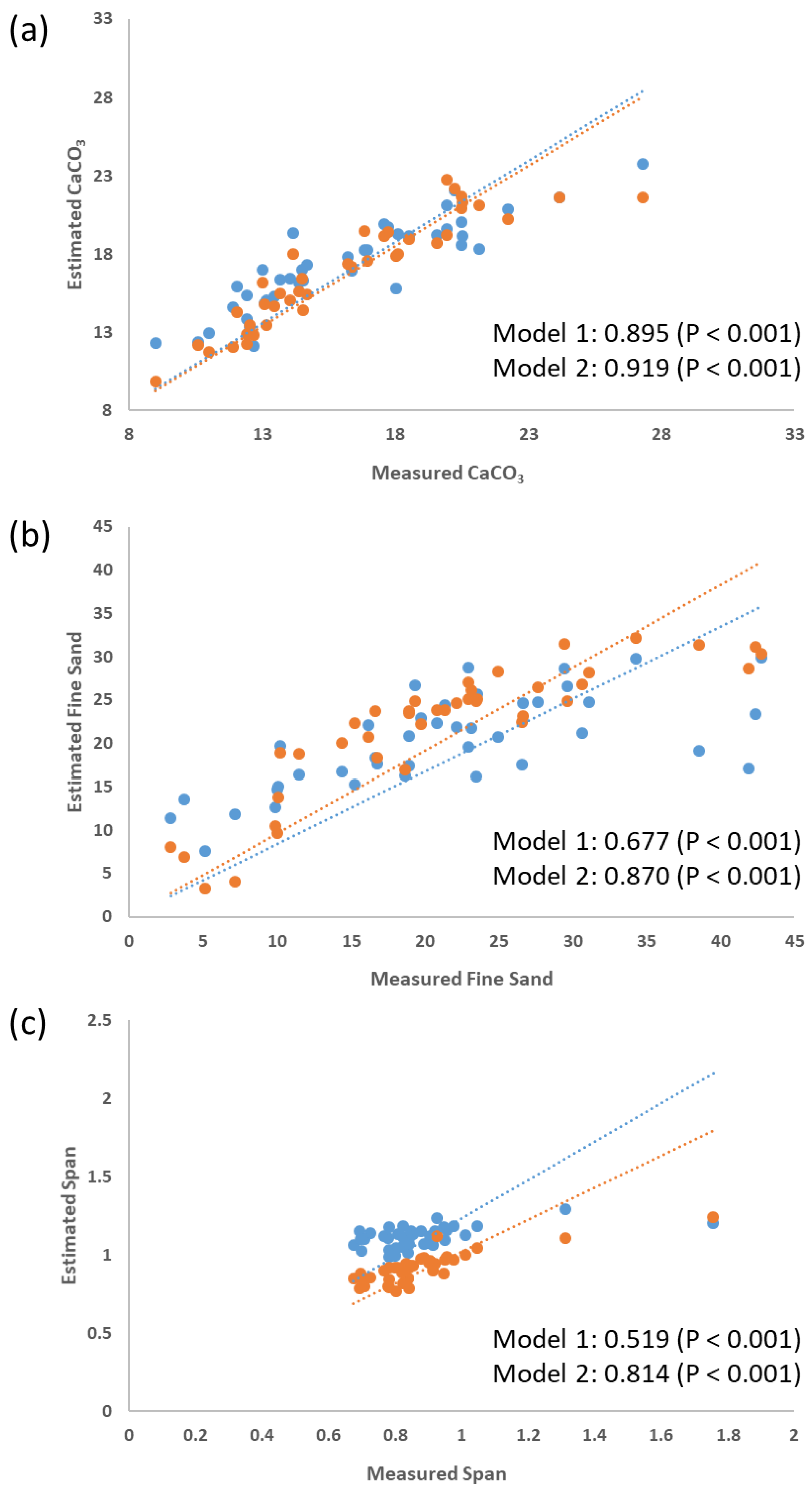
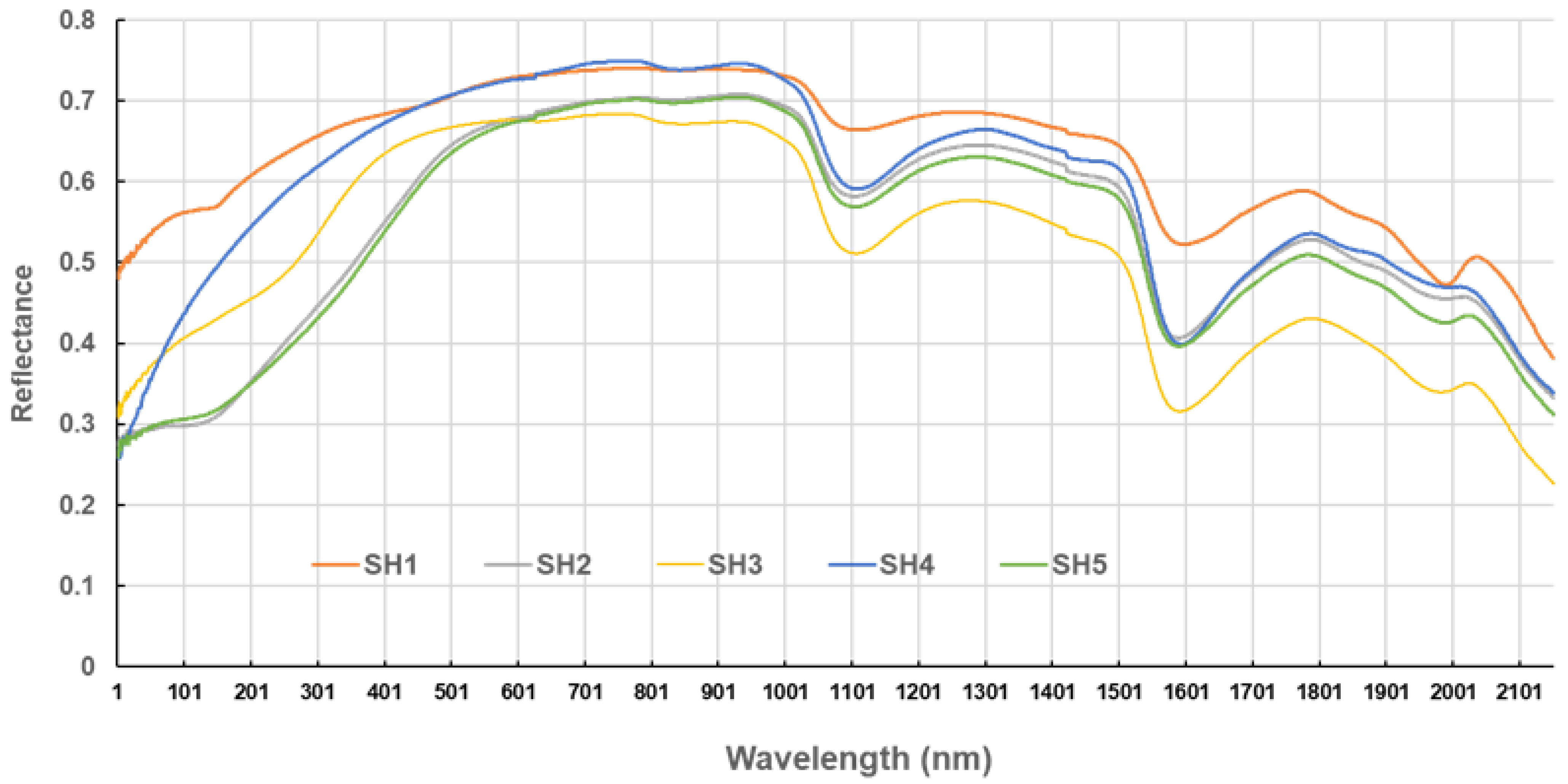
3.3. Spectral Analysis of Sediment Samples
4. Discussion
5. Conclusions
Author Contributions
Funding
Institutional Review Board Statement
Informed Consent Statement
Data Availability Statement
Conflicts of Interest
References
- De Lange, W.P.; Healy, T.R.; Darlan, Y. Reproducibility of sieve and settling tube textural determinations for sand-sized beach sediment. J. Coast. Res. 1997, 13, 73–80. [Google Scholar]
- Kasper-Zubillaga, J.J.; Ortiz-Zamora, G.; Dickinson, W.W.; Urrutia-Fucugauchi, J.; Soler-Arechalde, A.M. Textural and compositional controls on modern beach and dune sands, New Zealand. Earth Surf. Proc. Landf. 2007, 32, 366–389. [Google Scholar] [CrossRef]
- Kwarteng, A.Y.; Al-Hatrushi, S.M.; Illenberger, W.K.; McLachlan, A. Grain size and mineralogy of Al Batinah beach sediments, Sultanate of Oman. Arab. J. Geosci. 2016, 9, 557. [Google Scholar] [CrossRef]
- Hallin, C.; Almström, B.; Larson, M.; Hanson, H. Longshore transport variability of beach face grain size: Implications for dune evolution. J. Coastal Res. 2019, 35, 751–764. [Google Scholar] [CrossRef] [Green Version]
- Pyökäri, M. Beach Sediments of Crete: Texture, Composition, Roundness, Source and Transport. J. Coast. Res. 1999, 15, 537–553. [Google Scholar]
- Smith, D.A.; Cheung, K.F. Empirical relationships for grain size parameters of calcareous sand on Oahu, Hawaii. J. Coast. Res. 2002, 18, 82–93. [Google Scholar]
- Alsharhan, A.S.; El-Sammak, A.A. Grain size analysis and characterization of sedimentary environments of the United Arab Emirates coastal area. J. Coast. Res. 2004, 20, 464–477. [Google Scholar] [CrossRef]
- Deidun, A.; Gauci, R.; Schembri, J.A.; Šegina, E.; Gauci, A.; Gianni, J.; Gutierrez, J.A.; Sciberras, A.; Sciberras, J. Comparative median grain size assessment through three different techniques for sandy beach deposits on the Maltese Islands (Central Mediterranean). J. Coast. Res. 2013, 65, 1757–1761. [Google Scholar] [CrossRef]
- Poizot, E.; Anfuso, G.; Méar, Y.; Bellido, C. Confirmation of beach accretion by grain-size trend analysis: Camposoto beach, Cádiz, SW Spain. Geo-Mar. Lett. 2013, 33, 263–272. [Google Scholar] [CrossRef]
- Choi, T.J.; Choi, J.Y.; Park, J.Y.; Um, H.Y.; Choi, J.H. The Effects of Nourishments Using the Grain-Size Trend Analysis on the Intertidal Zone at a Sandy Macrotidal Beach. J. Coast. Res. 2018, 85, 426–430. [Google Scholar] [CrossRef]
- Gunaratna, T.; Suzuki, T.; Yanagishima, S. Cross-shore grain size and sorting patterns for the bed profile variation at a dissipative beach: Hasaki Coast, Japan. Mar. Geol. 2019, 407, 111–120. [Google Scholar] [CrossRef]
- Pedreros, R.; Howa, H.L.; Michel, D. Application of grain size trend analysis for the determination of sediment transport pathways in intertidal areas. Mar. Geol. 1996, 135, 35–49. [Google Scholar] [CrossRef] [Green Version]
- Edwards, A.C. Grain Size and Sorting in Modern Beach Sands. J. Coast. Res. 2001, 17, 38–52. [Google Scholar]
- Gallagher, E.L.; MacMahan, J.; Reniers, A.J.H.M.; Brown, J.; Thornton, E.B. Grain size variability on a rip-channeled beach. Mar. Geol. 2011, 287, 43–53. [Google Scholar] [CrossRef]
- Pradhan, U.K.; Sahoo, R.K.; Pradhan, S.; Mohany, P.K.; Mishra, P. Textural Analysis of Coastal Sediments along East Coast of India. J. Geol. Soc. India 2020, 95, 67–74. [Google Scholar] [CrossRef]
- Deronde, B.; Kempeneers, P.; Forster, R.M. Imaging spectroscopy as a tool to study sediment characteristics on a tidal sandbank in the Westerschelde. Estuar. Coast. Shelf Sci. 2006, 69, 580–590. [Google Scholar] [CrossRef]
- Castillo, E.; Pereda, R.; de Luis, J.M.; Medina, R.; Viguri, J. Sediment grain size estimation using airborne remote sensing, field sampling, and robust statistic. Environ. Monit. Assess. 2011, 181, 431–444. [Google Scholar] [CrossRef]
- Manzo, C.; Valentini, E.; Taramelli, A.; Filipponi, F.; Disperati, L. Spectral characterization of coastal sediments using Field Spectral Libraries, Airborne Hyperspectral Images and Topographic LiDAR Data (FHyL). Int. J. Appl. Earth Obs. Geoinf. 2015, 36, 54–68. [Google Scholar] [CrossRef]
- Ibrahim, E.; Kim, W.; Crawford, M.; Monbaliu, J. A regression approach to the mapping of bio-physical characteristics of surface sediment using in situ and airborne hyperspectral acquisitions. Ocean. Dyn. 2017, 67, 299–316. [Google Scholar] [CrossRef]
- Smit, Y.; Ruessink, G.; Brakenhoff, L.B.; Donker, J.J.A. Measuring spatial and temporal variation in surface moisture on a coastal beach with a near-infrared terrestrial laser scanner. Aeolian Res. 2018, 31, 19–27. [Google Scholar] [CrossRef]
- Kim, K.-L.; Kim, B.-J.; Lee, Y.-K.; Ryu, J.-H. Generation of a Large-Scale Surface Sediment Classification Map Using Unmanned Aerial Vehicle (UAV) Data: A Case Study at the Hwang-do Tidal Flat, Korea. Remote Sens. 2019, 11, 29. [Google Scholar] [CrossRef] [Green Version]
- Jacq, K.; Giguet-Covex, C.; Sabatier, P.; Perrette, Y.; Fanget, B.; Coquin, D.; Debret, M.; Arnaud, F. High-resolution grain size distribution of sediment core with hyperspectral imaging. Sediment. Geol. 2019, 393–394, 105536. [Google Scholar] [CrossRef]
- Ghanbari, H.; Jacques, O.; Adaïmé, M.É.; Gregory-Eaves, I.; Antoniades, D. Remote Sensing of Lake Sediment Core Particle Size Using Hyperspectral Image Analysis. Remote Sens. 2020, 12, 3850. [Google Scholar] [CrossRef]
- Zander, P.D.; Wienhues, G.; Grosjean, M. Scanning Hyperspectral Imaging for In Situ Biogeochemical Analysis of Lake Sediment Cores: Review of Recent Developments. J. Imaging 2022, 8, 58. [Google Scholar] [CrossRef]
- Ryu, J.-H.; Na, Y.-H.; Won, J.-S.; Doerffer, R. A critical grain size for Landsat ETM+ investigations into intertidal sediments: A case study of the Gomso tidal flats, Korea. Estuar. Coast. Shelf Sci. 2004, 60, 491–502. [Google Scholar] [CrossRef]
- Small, C.; Steckler, M.; Seeber, L.; Akhter, S.H.; Goodbred, S., Jr.; Mia, B.; Imam, B. Spectroscopy of sediments in the Ganges–Brahmaputra delta: Spectral effects of moisture, grain size and lithology. Remote Sens. Environ. 2009, 113, 342–361. [Google Scholar] [CrossRef]
- Legleiter, C.J.; Stegman, T.K.; Overstreet, B.T. Spectrally based mapping of riverbed composition. Geomorphology 2016, 264, 61–79. [Google Scholar] [CrossRef] [Green Version]
- Ciampalini, A.; Consoloni, I.; Salvatici, T.; Di Traglia, F.; Fidolini, F.; Sarti, G.; Moretti, S. Characterization of coastal environment by means of hyper- and multispectral techniques. Appl. Geogr. 2015, 57, 120–132. [Google Scholar] [CrossRef]
- Rejith, R.G.; Sundararajan, M.; Gnanappazham, L.; Loveson, V.J. Satellite-based spectral mapping (ASTER and Landsat data) of mineralogical signatures of beach sediments: A precursor insight. Geocarto Int. 2022, 1–24, in press. [Google Scholar] [CrossRef]
- Park, N.-W.; Jang, D.-H.; Chi, K.-H. Integration of IKONOS imagery for geostatistical mapping of sediment grain size at Baramarae beach, Korea. Int. J. Remote Sens. 2009, 30, 5703–5724. [Google Scholar] [CrossRef]
- Williams, K.K.; Greeley, R. Laboratory and field measurements of the modification of radar backscatter by sand. Remote Sens. Environ. 2004, 89, 29–40. [Google Scholar] [CrossRef]
- Van der Wal, D.; Herman, P.M.J. Regression-based synergy of optical, shortwave infrared and microwave remote sensing for monitoring the grain-size of intertidal sediments. Remote Sens. Environ. 2007, 111, 89–106. [Google Scholar] [CrossRef]
- Rainey, M.P.; Tyler, A.N.; Gilvear, D.J.; Bryant, R.G.; McDonald, P. Mapping intertidal estuarine sediment grain size distributions through airborne remote sensing. Remote Sens. Environ. 2003, 86, 480–490. [Google Scholar] [CrossRef]
- Choi, J.K.; Ryu, J.H.; Eom, J. Integration of spatial variables derived from remotely sensed data for the mapping of the tidal surface sediment distribution. J. Coast. Res. 2011, 64, 1653–1657. [Google Scholar]
- Ibrahim, E.; Monbaliu, J. Suitability of spaceborne multispectral data for inter-tidal sediment characterization: A case study. Estuar. Coast. Shelf Sci. 2011, 92, 437–445. [Google Scholar] [CrossRef]
- Park, N.-W. Geostatistical integration of field measurements and multi-sensor remote sensing images for spatial prediction of grain size of intertidal surface sediments. J. Coast. Res. 2019, SI90, 190–196. [Google Scholar] [CrossRef]
- Wepener, V.; Degger, N. South Africa. In World Seas: An Environmental Evaluation: Volume II: The Indian Ocean to the Pacific, 2nd ed.; Sheppard, C., Ed.; Elsevier: Amsterdam, The Netherlands, 2019; pp. 101–119. [Google Scholar]
- Meeuwis, J.; van Rensburg, P.A.J. Logarithmic spiral coastlines: The northern Zululand coastline. S. Afr. Geogr. J. 1986, 68, 18–44. [Google Scholar] [CrossRef]
- Knight, J.; Burningham, H. The morphodynamics of transverse dunes on the coast of South Africa. Geo-Mar. Lett. 2021, 41, 47. [Google Scholar] [CrossRef]
- Roberts, D.L.; Botha, G.A.; Maud, R.R.; Pether, J. Coastal Cenozoic Deposits. In The Geology of South Africa; Johnson, M.R., Anhaeusser, C.R., Thomas, R.J., Eds.; Geological Society of South Africa/Council for Geoscience: Johannesburg/Pretoria, South Africa, 2006; pp. 605–628. [Google Scholar]
- Claassen, D. Geographical controls on sediment accretion of the Cenozoic Algoa Group between Oyster Bay and St. Francis, Eastern Cape coastline, South Africa. S. Afr. J. Geol. 2014, 117, 109–128. [Google Scholar] [CrossRef]
- Knight, J. The late Quaternary stratigraphy of coastal dunes and associated deposits in South Africa. S. Afr. J. Geol. 2021, 124, 995–1006. [Google Scholar] [CrossRef]
- Butzer, K.W.; Helgren, D.M. Late Cenozoic evolution of the Cape coast between Knysna and Cape St. Francis, South Africa. Quat. Res. 1972, 2, 143–169. [Google Scholar] [CrossRef]
- Rossel, R.A.V.; McBratney, A.B. Laboratory evaluation of a proximal sensing technique for simultaneous measurement of soil clay and water content. Geoderma 1998, 85, 19–39. [Google Scholar] [CrossRef]
- Schumann, E.H.; Illenberger, W.K.; Goschen, W.S. Surface winds over Algoa Bay, South Africa. S. Afr. J. Sci. 1991, 87, 202–207. [Google Scholar]
- Carter, R.W.G. Some problems associated with the analysis and interpretation of mixed carbonate and quartz beach sands, illustrated by examples from north-west Ireland. Sediment. Geol. 1982, 33, 35–56. [Google Scholar] [CrossRef]
- Fang, Q.; Hong, H.; Zhao, L.; Kukolich, S.; Yin, K.; Wang, C. Visible and Near-Infrared Reflectance Spectroscopy for Investigating Soil Mineralogy: A Review. J. Spectroscop. 2018, 2018, 3168974. [Google Scholar] [CrossRef]
- Lubke, R.A.; Sugden, J. Short-term change in mobile dunes at Port Alfred, South Africa. Environ. Manag. 1990, 14, 209–220. [Google Scholar] [CrossRef]
- Knight, J.; Burningham, H. Sand dunes and ventifacts on the coast of South Africa. Aeolian Res. 2019, 37, 44–58. [Google Scholar] [CrossRef]
- Harmse, J.T. Trend surface analysis of aeolian sand movement on the southwest African coast. S. Afr. Geogr. J. 1985, 67, 31–39. [Google Scholar] [CrossRef]
- Illenberger, W.K. Variations of sediment dynamics in Algoa Bay during the Holocene. S. Afr. J. Sci. 1993, 89, 187–196. [Google Scholar]
- Çelikoğlu, Y.; Yüksel, Y.; Kabdaşlı, M.S. Cross-shore sorting on a beach under wave action. J. Coast. Res. 2006, 22, 487–501. [Google Scholar] [CrossRef]
- Olivier, M.J.; Garland, G.G. Short-term monitoring of foredune formation on the east coast of South Africa. Earth Surf. Proc. Landf. 2003, 28, 1143–1155. [Google Scholar] [CrossRef]
- Bandfield, J.L.; Edgett, K.S.; Christensen, P.R. Spectroscopic study of the Moses Lake dune field, Washington: Determination of compositional distributions and source lithologies. J. Geophys. Res. 2002, 107, 5092. [Google Scholar] [CrossRef] [Green Version]
- Sadiq, A.; Howari, F. Remote Sensing and Spectral Characteristics of Desert Sand from Qatar Peninsula, Arabian/Persian Gulf. Remote Sens. 2009, 1, 915–933. [Google Scholar] [CrossRef] [Green Version]
- Moshtaghi, M.; Knaeps, E.; Sterckx, S.; Garaba, S.; Meire, D. Spectral reflectance of marine macroplastics in the VNIR and SWIR measured in a controlled environment. Sci. Rep. 2021, 11, 5436. [Google Scholar] [CrossRef] [PubMed]


| Sample # | Location Code | Lat | Long | Elevation (m asl) | D10 (Microns) | D50 (Microns) | D90 (Microns) | Kurtosis | Skewness | CaCO3 (%) | Fine sand (%) | Medium Sand (%) | Coarse Sand (%) | Very Coarse Sand (%) |
|---|---|---|---|---|---|---|---|---|---|---|---|---|---|---|
| 006 | BEC | −34.171938 | 24.642923 | 4.211 | 209 | 315 | 478 | 0.95 | 0.00 | 18.83 | 24.34 | 68.06 | 7.59 | 0.00 |
| 007 | BET | −34.171984 | 24.642668 | 2.048 | 220 | 340 | 528 | 0.95 | −0.01 | 13.78 | 18.57 | 68.07 | 13.35 | 0.00 |
| 008 | SLT | −34.172052 | 24.642489 | 4.932 | 199 | 289 | 421 | 0.97 | 0.00 | 10.40 | 31.47 | 65.92 | 2.61 | 0.00 |
| 009 | BES | −34.172016 | 24.642389 | 8.777 | 302 | 488 | 804 | 0.95 | −0.02 | 21.40 | 3.16 | 49.36 | 44.73 | 2.75 |
| 010 | BET | −34.172011 | 24.642128 | 7.816 | 226 | 350 | 547 | 0.96 | −0.01 | 13.69 | 16.50 | 68.12 | 15.38 | 0.00 |
| 011 | BET | −34.171679 | 24.641879 | 5.172 | 201 | 323 | 538 | 0.98 | −0.04 | 16.20 | 25.10 | 61.41 | 11.89 | 0.88 |
| 012 | BEC | −34.171517 | 24.642276 | 11.661 | 204 | 307 | 465 | 0.94 | 0.00 | 17.04 | 26.57 | 66.99 | 6.44 | 0.00 |
| 013 | BEI | −34.171702 | 24.642363 | 11.661 | 198 | 288 | 420 | 0.97 | 0.00 | 9.89 | 31.79 | 65.61 | 2.60 | 0.00 |
| 014 | CRS | −34.171690 | 24.642476 | 9.739 | 279 | 442 | 715 | 0.96 | −0.02 | 21.98 | 5.30 | 57.36 | 36.33 | 1.01 |
| 015 | SLT | −34.171666 | 24.642576 | 8.296 | 203 | 303 | 453 | 0.95 | −0.01 | 12.30 | 27.39 | 67.18 | 5.43 | 0.00 |
| 016 | BET | −34.171933 | 24.643384 | 6.134 | 220 | 340 | 529 | 0.95 | −0.01 | 14.58 | 18.69 | 67.89 | 13.42 | 0.00 |
| 017 | BEC | −34.172137 | 24.643902 | 9.739 | 254 | 392 | 609 | 0.96 | −0.01 | 19.09 | 9.01 | 66.63 | 24.29 | 0.06 |
| 018 | BEC | −34.171929 | 24.643805 | 7.816 | 207 | 311 | 470 | 0.95 | −0.01 | 16.44 | 25.28 | 67.90 | 6.82 | 0.00 |
| 019 | CRS | −34.171833 | 24.644029 | 12.382 | 248 | 382 | 589 | 0.95 | −0.01 | 16.60 | 10.45 | 67.69 | 21.83 | 0.03 |
| 020 | BET | −34.171374 | 24.643891 | 5.893 | 189 | 287 | 440 | 0.96 | −0.01 | 12.66 | 34.09 | 61.50 | 4.41 | 0.00 |
| 021 | BEC | −34.171120 | 24.643643 | 9.017 | 214 | 321 | 485 | 0.96 | 0.00 | 19.35 | 22.28 | 69.53 | 8.19 | 0.00 |
| 022 | INR | −34.171363 | 24.643649 | 7.095 | 228 | 374 | 631 | 0.96 | −0.03 | 18.76 | 15.15 | 60.88 | 23.40 | 0.50 |
| 023 | INR | −34.171499 | 24.643289 | 9.498 | 217 | 351 | 583 | 0.97 | −0.04 | 16.97 | 18.85 | 62.41 | 17.85 | 0.56 |
| 024 | RAS | −34.171600 | 24.642989 | 9.979 | 218 | 343 | 543 | 0.96 | −0.01 | 16.90 | 19.06 | 66.14 | 14.79 | 0.00 |
| 025 | RAS | −34.171869 | 24.643010 | 6.134 | 204 | 318 | 503 | 0.95 | −0.02 | 12.93 | 25.10 | 64.54 | 10.36 | 0.00 |
| 026 | BAB | −34.172203 | 24.642861 | 8.537 | 199 | 302 | 459 | 0.95 | −0.01 | 16.21 | 28.53 | 65.40 | 6.06 | 0.00 |
| 027 | BAT | −34.171951 | 24.642091 | 1.087 | 219 | 339 | 528 | 0.95 | −0.01 | 16.78 | 19.19 | 67.50 | 13.30 | 0.00 |
| 028 | BAT | −34.171980 | 24.641696 | 6.134 | 226 | 372 | 631 | 0.97 | −0.03 | 21.13 | 15.64 | 60.75 | 22.84 | 0.70 |
| 029 | BAC | −34.171961 | 24.641441 | 7.095 | 211 | 314 | 472 | 0.95 | 0.00 | 14.73 | 23.86 | 69.23 | 6.91 | 0.00 |
| 030 | BAT | −34.171942 | 24.641264 | 5.893 | 200 | 311 | 490 | 0.96 | −0.02 | 13.61 | 26.92 | 64.19 | 8.89 | 0.00 |
| 031 | BEC | −34.171955 | 24.641151 | 5.653 | 221 | 344 | 530 | 0.95 | 0.01 | 19.22 | 18.14 | 68.19 | 13.67 | 0.00 |
| 032 | BES | −34.171565 | 24.641033 | 6.134 | 261 | 416 | 669 | 0.95 | −0.01 | 20.08 | 7.88 | 60.64 | 30.94 | 0.54 |
| 033 | BEC | −34.171277 | 24.640809 | 3.250 | 187 | 274 | 402 | 0.95 | 0.00 | 22.41 | 38.30 | 59.87 | 1.83 | 0.00 |
| 034 | BAT | −34.171125 | 24.640865 | 8.296 | 202 | 307 | 466 | 0.95 | 0.00 | 17.58 | 27.05 | 66.48 | 6.47 | 0.00 |
| 035 | RAS | −34.171038 | 24.640841 | 7.816 | 219 | 336 | 514 | 0.95 | 0.00 | 12.13 | 19.35 | 68.71 | 11.94 | 0.00 |
| 036 | BAC | −34.171123 | 24.640999 | 5.653 | 210 | 316 | 481 | 0.96 | 0.00 | 20.16 | 23.92 | 68.25 | 7.83 | 0.00 |
| 037 | BAT | −34.171193 | 24.641281 | 0.125 | 254 | 466 | 1020 | 1.06 | −0.13 | 26.58 | 9.31 | 46.06 | 34.29 | 8.86 |
| 038 | BAC | −34.171223 | 24.641788 | 4.692 | 191 | 284 | 425 | 0.96 | 0.00 | 19.23 | 34.60 | 62.35 | 3.04 | 0.00 |
| 039 | BAR | −34.171376 | 24.641656 | 6.374 | 180 | 264 | 388 | 0.96 | −0.01 | 12.38 | 42.81 | 55.96 | 1.22 | 0.00 |
| 040 | BAT | −34.171621 | 24.641768 | 4.451 | 213 | 327 | 508 | 0.95 | −0.01 | 14.72 | 21.97 | 67.04 | 11.00 | 0.00 |
| 041 | BAC | −34.171713 | 24.641632 | 7.335 | 239 | 366 | 565 | 0.95 | −0.01 | 18.44 | 13.12 | 68.71 | 18.16 | 0.00 |
| 042 | BAB | −34.172004 | 24.639971 | 1.808 | 225 | 363 | 589 | 0.95 | −0.01 | 14.92 | 16.26 | 63.45 | 20.20 | 0.09 |
| 043 | BAC | −34.171775 | 24.639973 | 6.854 | 235 | 340 | 488 | 0.95 | 0.02 | 18.42 | 14.63 | 77.03 | 8.34 | 0.00 |
| 044 | BAC | −34.171648 | 24.639890 | 9.258 | 219 | 328 | 494 | 0.96 | −0.01 | 15.84 | 19.78 | 71.01 | 9.20 | 0.00 |
| 045 | BAS | −34.171388 | 24.639973 | 8.296 | 253 | 393 | 611 | 0.96 | −0.01 | 19.06 | 9.30 | 66.09 | 24.55 | 0.06 |
| 046 | BAC | −34.171020 | 24.639773 | 10.700 | 213 | 322 | 490 | 0.96 | 0.00 | 19.00 | 22.25 | 68.96 | 8.79 | 0.00 |
| 047 | BAS | −34.171247 | 24.640023 | 5.413 | 203 | 310 | 481 | 0.96 | −0.02 | 10.27 | 26.40 | 65.66 | 7.94 | 0.00 |
| 048 | RAT | −34.171330 | 24.640202 | 6.374 | 206 | 318 | 495 | 0.95 | −0.01 | 15.96 | 24.55 | 66.09 | 9.36 | 0.00 |
| 049 | RAS | −34.171756 | 24.640200 | 6.134 | 239 | 391 | 671 | 0.97 | −0.05 | 17.20 | 12.77 | 59.31 | 26.55 | 1.37 |
| 050 | BAC | −34.171887 | 24.640709 | 5.653 | 222 | 350 | 556 | 0.96 | −0.01 | 17.06 | 17.60 | 66.07 | 16.32 | 0.01 |
| 051 | BAC | −34.171602 | 24.640481 | 3.730 | 217 | 359 | 625 | 0.99 | −0.06 | 20.63 | 18.40 | 59.74 | 20.10 | 1.31 |
| 052 | RAT | −34.171232 | 24.640564 | 3.971 | 176 | 248 | 347 | 0.96 | −0.01 | 15.27 | 51.21 | 48.62 | 0.17 | 0.00 |
| 053 | RAT | −34.171263 | 24.640642 | 7.816 | 192 | 274 | 391 | 0.96 | 0.00 | 16.61 | 37.27 | 61.61 | 1.12 | 0.00 |
| 054 | INT | −34.171117 | 24.640536 | 6.374 | 201 | 300 | 448 | 0.96 | 0.00 | 15.57 | 28.33 | 66.84 | 4.84 | 0.00 |
| 055 | BAT | −34.171473 | 24.641231 | 5.893 | 207 | 319 | 498 | 0.95 | −0.01 | 14.82 | 24.19 | 66.06 | 9.75 | 0.00 |
| 056 | BAT | −34.171814 | 24.641265 | 7.335 | 205 | 326 | 530 | 0.95 | −0.03 | 14.89 | 23.92 | 62.98 | 13.00 | 0.07 |
| 057 | BAB | −34.172157 | 24.641878 | 3.730 | 197 | 289 | 427 | 0.97 | 0.00 | 13.48 | 31.65 | 65.29 | 3.06 | 0.00 |
| 058 | BAB | −34.171930 | 24.639000 | 6.374 | 226 | 350 | 549 | 0.96 | −0.01 | 15.02 | 16.61 | 67.71 | 15.67 | 0.00 |
| 059 | CRI | −34.171679 | 24.639045 | 7.576 | 207 | 306 | 454 | 0.95 | −0.01 | 17.67 | 26.14 | 68.32 | 5.54 | 0.00 |
| 060 | BAC | −34.171248 | 24.639070 | 8.537 | 214 | 344 | 568 | 0.96 | −0.03 | 20.12 | 20.34 | 62.49 | 17.06 | 0.11 |
| 061 | BAC | −34.171124 | 24.639230 | 6.374 | 243 | 443 | 1240 | 1.09 | −0.25 | 24.65 | 11.32 | 46.87 | 27.58 | 11.11 |
| 062 | BAT | −34.171242 | 24.639314 | 0.606 | 195 | 291 | 438 | 0.96 | −0.01 | 9.97 | 31.81 | 64.08 | 4.11 | 0.00 |
| 063 | MAI | −34.171381 | 24.639556 | 5.893 | 219 | 345 | 551 | 0.96 | −0.02 | 17.32 | 18.71 | 65.64 | 15.63 | 0.01 |
| 064 | RAT | −34.171685 | 24.639376 | 4.451 | 217 | 354 | 620 | 1.00 | −0.07 | 19.63 | 18.90 | 60.14 | 18.94 | 1.53 |
| 065 | BAT | −34.171786 | 24.639684 | 7.816 | 216 | 329 | 504 | 0.96 | 0.00 | 16.76 | 20.70 | 68.83 | 10.47 | 0.00 |
| 066 | INT | −34.171465 | 24.639731 | 3.730 | 214 | 351 | 616 | 0.99 | −0.07 | 15.92 | 19.78 | 59.69 | 18.78 | 1.41 |
| 067 | INR | −34.170996 | 24.639434 | 13.103 | 208 | 324 | 510 | 0.95 | −0.01 | 18.77 | 23.52 | 65.21 | 11.27 | 0.00 |
| 068 | INS | −34.171154 | 24.640406 | 8.777 | 219 | 327 | 488 | 0.96 | 0.00 | 18.75 | 19.95 | 71.52 | 8.53 | 0.00 |
| 069 | CRI | −34.171594 | 24.629845 | −5.641 | 238 | 406 | 722 | 0.98 | −0.04 | 23.67 | 12.58 | 55.56 | 29.39 | 2.34 |
| 070 | CRI | −34.171147 | 24.630392 | 12.863 | 246 | 396 | 639 | 0.96 | 0.00 | 18.05 | 11.02 | 61.88 | 26.90 | 0.21 |
| 071 | CRI | −34.170616 | 24.630827 | 12.622 | 252 | 388 | 594 | 0.96 | 0.00 | 19.25 | 6.45 | 67.59 | 22.95 | 0.01 |
| 072 | CRS | −34.170290 | 24.631101 | 10.700 | 262 | 392 | 583 | 0.95 | 0.00 | 19.47 | 7.53 | 70.20 | 22.27 | 0.01 |
| 073 | BAR | −34.171394 | 24.631663 | 8.296 | 195 | 302 | 474 | 0.96 | −0.02 | 18.67 | 29.59 | 6.97 | 7.43 | 0.00 |
| 074 | BER | −34.172438 | 24.631051 | −0.354 | 223 | 334 | 498 | 0.96 | 0.00 | 14.11 | 18.15 | 72.14 | 9.72 | 0.00 |
| 075 | BAR | −34.170938 | 24.635953 | 6.134 | 220 | 358 | 581 | 0.95 | 0.00 | 22.10 | 17.65 | 62.85 | 19.47 | 0.03 |
| 076 | BAT | −34.171616 | 24.635743 | 10.459 | 196 | 287 | 423 | 0.97 | 0.00 | 11.41 | 32.60 | 64.59 | 2.81 | 0.00 |
| 077 | BAC | −34.171935 | 24.635784 | 4.692 | 215 | 331 | 512 | 0.95 | −0.01 | 17.54 | 20.85 | 67.59 | 11.56 | 0.00 |
| 078 | BER | −34.172500 | 24.636502 | 5.653 | 219 | 337 | 521 | 0.95 | −0.01 | 14.71 | 19.23 | 68.12 | 12.65 | 0.00 |
| 079 | BAT | −34.171834 | 24.636919 | 8.537 | 241 | 361 | 545 | 0.96 | −0.01 | 13.34 | 12.68 | 71.64 | 15.68 | 0.00 |
| 080 | BAR | −34.171110 | 24.637048 | 8.777 | 213 | 343 | 562 | 0.96 | −0.02 | 20.47 | 20.49 | 62.92 | 16.54 | 0.05 |
| 081 | CRS | −34.170847 | 24.638189 | 13.584 | 253 | 432 | 808 | 0.99 | −0.08 | 27.25 | 9.38 | 53.07 | 33.00 | 4.49 |
| 082 | BAB | −34.171690 | 24.638149 | 4.932 | 234 | 354 | 530 | 0.94 | 0.01 | 15.92 | 14.35 | 71.73 | 13.92 | 0.00 |
| 083 | BAB | −34.172336 | 24.638428 | 7.335 | 239 | 429 | 865 | 0.99 | −0.10 | 25.33 | 12.28 | 49.43 | 31.89 | 6.09 |
| 084 | BAI | −34.171595 | 24.638524 | 2.048 | 197 | 294 | 442 | 0.96 | −0.01 | 20.45 | 30.71 | 64.88 | 4.41 | 0.00 |
| 085 | INR | −34.171029 | 24.638807 | 10.459 | 236 | 371 | 584 | 0.94 | −0.01 | 20.34 | 13.49 | 65.94 | 20.54 | 0.04 |
| 086 | CRI | −34.170733 | 24.638722 | 13.584 | 190 | 275 | 396 | 0.96 | 0.00 | 15.50 | 37.34 | 61.22 | 1.44 | 0.00 |
| 087 | BET | −34.172485 | 24.640166 | 5.413 | 196 | 281 | 400 | 0.96 | 0.00 | 12.29 | 34.09 | 64.39 | 1.51 | 0.00 |
| 088 | BET | −34.172541 | 24.641305 | 5.653 | 234 | 385 | 642 | 0.95 | −0.01 | 19.48 | 13.60 | 60.30 | 25.74 | 0.36 |
| 089 | BET | −34.172570 | 24.642399 | 1.567 | 275 | 436 | 699 | 0.95 | −0.01 | 19.73 | 5.96 | 58.23 | 35.16 | 0.65 |
| 090 | BET | −34.172851 | 24.643780 | 5.893 | 336 | 517 | 801 | 0.96 | −0.01 | 24.00 | 1.02 | 45.16 | 51.74 | 2.09 |
| 091 | BAB | −34.172520 | 24.644298 | 4.451 | 204 | 296 | 430 | 0.96 | 0.00 | 12.54 | 28.48 | 68.45 | 3.07 | 0.00 |
| 092 | BAS | −34.172002 | 24.644281 | 6.134 | 193 | 272 | 385 | 0.96 | 0.00 | 8.26 | 37.81 | 61.32 | 0.87 | 0.00 |
| 093 | BAS | −34.171981 | 24.644318 | 7.335 | 200 | 297 | 443 | 0.96 | −0.01 | 8.86 | 29.30 | 66.25 | 4.45 | 0.00 |
| 094 | BAC | −34.171375 | 24.644495 | 9.739 | 256 | 403 | 643 | 0.96 | −0.01 | 17.99 | 8.82 | 63.06 | 27.87 | 0.25 |
| 095 | BAR | −34.170761 | 24.644425 | 8.296 | 224 | 338 | 511 | 0.96 | −0.01 | 17.33 | 17.64 | 70.80 | 11.57 | 0.00 |
| 096 | BAT | −34.171188 | 24.644581 | 6.614 | 215 | 338 | 553 | 0.97 | −0.04 | 13.67 | 20.53 | 64.14 | 14.33 | 0.54 |
| 097 | BAI | −34.171828 | 24.644937 | 7.816 | 213 | 330 | 518 | 0.95 | −0.01 | 13.86 | 21.65 | 66.14 | 12.21 | 0.00 |
| 098 | BAT | −34.172261 | 24.644822 | 5.413 | 201 | 289 | 416 | 0.96 | 0.00 | 8.22 | 30.99 | 66.75 | 2.26 | 0.00 |
| 099 | BAB | −34.172608 | 24.645214 | 6.134 | 217 | 329 | 504 | 0.96 | −0.01 | 14.48 | 20.40 | 69.15 | 10.46 | 0.00 |
| 100 | BER | −34.172899 | 24.645462 | 4.451 | 249 | 375 | 565 | 0.96 | 0.00 | 13.02 | 10.23 | 71.10 | 18.67 | 0.00 |
| 101 | BAC | −34.172244 | 24.645432 | 8.056 | 235 | 353 | 535 | 0.95 | −0.01 | 18.51 | 14.37 | 71.23 | 14.40 | 0.00 |
| 102 | BAC | −34.171919 | 24.645569 | 9.258 | 225 | 349 | 541 | 0.96 | 0.00 | 21.15 | 16.78 | 68.35 | 14.88 | 0.00 |
| 103 | BAS | −34.171447 | 24.645305 | 10.700 | 294 | 479 | 796 | 0.96 | −0.02 | 22.23 | 3.75 | 50.59 | 42.96 | 2.71 |
| 104 | BAT | −34.171306 | 24.645469 | 7.576 | 227 | 355 | 564 | 0.96 | −0.02 | 14.56 | 16.22 | 66.43 | 17.32 | 0.02 |
| 105 | RAS | -34.296997 | 24.645517 | 10.700 | 219 | 340 | 532 | 0.95 | −0.01 | 18.10 | 18.95 | 67.40 | 13.65 | 0.00 |
| 106 | CRS | −34.170927 | 24.645926 | 10.459 | 250 | 444 | 1030 | 1.11 | −0.19 | 24.17 | 9.93 | 48.97 | 30.52 | 8.51 |
| 107 | SLT | −34.170939 | 24.645957 | 9.498 | 214 | 314 | 460 | 0.95 | 0.00 | 10.60 | 22.94 | 71.26 | 5.80 | 0.00 |
| 108 | CRR | −34.170890 | 24.646282 | 10.459 | 229 | 361 | 571 | 0.96 | 0.00 | 17.58 | 15.24 | 66.17 | 18.57 | 0.02 |
| 109 | CRR | −34.171110 | 24.646571 | 11.901 | 218 | 351 | 573 | 0.96 | −0.01 | 20.53 | 18.70 | 63.19 | 18.05 | 0.05 |
| 110 | CRT | −34.170858 | 24.646711 | 7.335 | 195 | 293 | 442 | 0.96 | 0.00 | 12.43 | 31.15 | 64.41 | 4.41 | 0.00 |
| 111 | CRS | −34.170820 | 24.646927 | 9.258 | 250 | 392 | 625 | 0.97 | −0.02 | 20.51 | 10.04 | 64.54 | 25.21 | 0.21 |
| 112 | CRT | −34.170819 | 24.647034 | 4.451 | 209 | 322 | 503 | 0.95 | −0.01 | 11.89 | 23.57 | 66.05 | 10.37 | 0.00 |
| 113 | CRR | −34.171350 | 24.647209 | 13.103 | 213 | 316 | 469 | 0.95 | 0.00 | 16.22 | 22.98 | 70.41 | 6.61 | 0.00 |
| 114 | RAS | −34.171908 | 24.647452 | 19.832 | 179 | 265 | 391 | 0.95 | 0.00 | 12.67 | 42.77 | 55.89 | 1.34 | 0.00 |
| 115 | CRR | −34.171724 | 24.647273 | 21.995 | 190 | 272 | 388 | 0.96 | 0.00 | 16.95 | 38.57 | 60.42 | 1.00 | 0.00 |
| 116 | BAC | −34.171782 | 24.646935 | 20.313 | 204 | 308 | 467 | 0.95 | −0.01 | 20.51 | 26.57 | 66.85 | 6.58 | 0.00 |
| 117 | BAS | −34.171910 | 24.646599 | 12.622 | 200 | 295 | 437 | 0.96 | 0.00 | 12.42 | 29.66 | 66.46 | 3.88 | 0.00 |
| 118 | BAC | −34.171930 | 24.646544 | 17.910 | 220 | 327 | 489 | 0.96 | 0.00 | 18.03 | 19.74 | 71.69 | 8.57 | 0.00 |
| 119 | BAC | −34.172095 | 24.646437 | 12.622 | 244 | 372 | 571 | 0.96 | −0.01 | 19.95 | 11.50 | 69.24 | 19.25 | 0.01 |
| 120 | CRS | −34.171342 | 24.648271 | 4.451 | 197 | 280 | 393 | 0.96 | 0.00 | 8.99 | 34.25 | 64.66 | 1.09 | 0.00 |
| 121 | CRS | −34.171682 | 24.648521 | 11.421 | 202 | 309 | 476 | 0.95 | −0.01 | 13.09 | 26.68 | 65.85 | 7.47 | 0.00 |
| 122 | CRS | −34.171691 | 24.648334 | 13.824 | 203 | 288 | 407 | 0.96 | 0.00 | 16.36 | 30.69 | 67.61 | 1.70 | 0.00 |
| 123 | CRS | −34.171218 | 24.648048 | 13.103 | 266 | 422 | 678 | 0.94 | −0.01 | 19.95 | 7.19 | 60.04 | 32.25 | 0.53 |
| 124 | CRS | −34.171781 | 24.647969 | 22.716 | 189 | 264 | 372 | 0.96 | 0.01 | 19.57 | 41.90 | 57.63 | 0.47 | 0.00 |
| 125 | CRS | −34.172032 | 24.647721 | 16.948 | 188 | 263 | 371 | 0.96 | 0.01 | 12.07 | 42.40 | 57.15 | 0.45 | 0.00 |
| 126 | INR | −34.172320 | 24.647587 | 12.863 | 201 | 295 | 432 | 0.96 | 0.00 | 11.01 | 29.49 | 67.17 | 3.34 | 0.00 |
| 127 | CRS | −34.172309 | 24.647358 | 16.468 | 301 | 466 | 733 | 0.96 | −0.02 | 20.23 | 2.83 | 54.98 | 41.19 | 1.09 |
| 128 | BAT | −34.172380 | 24.647111 | 9.979 | 214 | 330 | 512 | 0.95 | −0.01 | 13.46 | 21.34 | 67.11 | 11.56 | 0.00 |
| 129 | BAC | −34.172293 | 24.646948 | 12.382 | 213 | 313 | 458 | 0.95 | 0.00 | 17.74 | 23.50 | 70.80 | 5.70 | 0.00 |
| 130 | BAT | −34.172286 | 24.646591 | 10.940 | 217 | 325 | 488 | 0.96 | 0.00 | 14.41 | 20.83 | 70.66 | 8.52 | 0.00 |
| 131 | BAC | −34.172367 | 24.646384 | 10.459 | 212 | 317 | 478 | 0.96 | 0.00 | 14.05 | 23.17 | 69.29 | 7.54 | 0.00 |
| 132 | BAB | −34.172595 | 24.646253 | 4.932 | 220 | 330 | 497 | 0.96 | 0.00 | 12.53 | 19.34 | 71.00 | 9.66 | 0.00 |
| 133 | BAB | −34.172955 | 24.646132 | 6.854 | 285 | 500 | 941 | 0.96 | −0.06 | 27.29 | 5.15 | 44.90 | 41.99 | 7.86 |
| 134 | BAB | −34.172679 | 24.646923 | 4.692 | 208 | 312 | 471 | 0.95 | −0.01 | 14.71 | 25.00 | 68.10 | 6.90 | 0.00 |
| 135 | BER | −34.173066 | 24.647486 | 6.614 | 250 | 373 | 558 | 0.96 | 0.00 | 14.17 | 10.10 | 72.04 | 17.87 | 0.00 |
| 136 | BAB | −34.172787 | 24.647920 | 5.172 | 216 | 316 | 463 | 0.96 | 0.00 | 13.70 | 22.17 | 71.79 | 6.04 | 0.00 |
| 137 | BAT | −34.172667 | 24.648487 | 3.490 | 221 | 331 | 494 | 0.96 | 0.00 | 14.50 | 18.94 | 71.83 | 9.24 | 0.00 |
| 138 | CRS | −34.172431 | 24.648988 | 6.614 | 229 | 333 | 485 | 0.96 | 0.00 | 16.86 | 16.69 | 75.25 | 8.06 | 0.00 |
| 139 | CRT | −34.172160 | 24.649022 | 4.451 | 210 | 293 | 408 | 0.97 | 0.01 | 13.16 | 27.66 | 70.87 | 1.48 | 0.00 |
| Location | D10 | D50 | D90 | CaCO3 | Fine Sand | Medium Sand | Coarse Sand | Very Coarse Sand |
|---|---|---|---|---|---|---|---|---|
| Backshore, beach | 0.0002 *** | 0.0004 *** | 0.0041 ** | 0.0455 * | 0.0120 * | 0.2313 | 0.0003 ** | 0.0148 * |
| Backshore, crest | 0.0265 * | 0.0318 * | 0.0475 * | 0.0005 ** | 0.1433 | 0.9129 | 0.0221 * | 0.1460 |
| Backshore, interdune | 0.8668 ^ | 0.5823 | 0.5154 | 0.9509 | 0.7269 | 0.8188 | 0.3936 | 0.8481 |
| Backshore, ramp | 0.1903 | 0.3554 | 0.6308 | 0.9566 | 0.0472 * | 0.5359 | 0.7108 | 0.9965 |
| Backshore, slip face | 0.4271 | 0.4077 | 0.5417 | 0.0813 ^ | 0.2634 | 0.7330 | 0.4244 | 0.9953 |
| Backshore, trough | 0.4534 | 0.8241 | 0.7296 | 0.0782 ^ | 0.3678 | 0.8872 | 0.9339 | 0.4140 |
| Beach, crest | 0.0113 * | 0.0144 * | 0.0817 ^ | 0.5547 | 0.0814 ^ | 0.1914 | 0.0192 * | 0.0967 ^ |
| Beach, interdune | 0.0038 ** | 0.0141 * | 0.0757 ^ | 0.1113 | 0.0803 ^ | 0.2343 | 0.0283 * | 0.0674 ^ |
| Beach, ramp | <0.0001 *** | <0.0001 *** | 0.0022 * | 0.0705 ^ | <0.0001 *** | 0.5811 | 0.0003 ** | 0.0241 * |
| Beach, slip face | 0.0069 ** | 0.0076 ** | 0.0365 * | 0.0067 ** | 0.0172 * | 0.3404 | 0.0081 * | 0.1989 |
| Beach, trough | <0.0001 * | <0.0001 *** | 0.0032 ** | 0.0002 *** | 0.0004 ** | 0.1425 | <0.0001 *** | 0.0379 * |
| Crest, interdune | 0.1626 | 0.3588 | 0.4935 | 0.0148 * | 0.5158 | 0.7372 | 0.4968 | 0.4123 |
| Crest, ramp | 0.0007 *** | 0.0036 ** | 0.0235 * | 0.0031 ** | 0.0004 ** | 0.5245 | 0.0163 * | 0.2081 |
| Crest, slip face | 0.0879 ^ | 0.0868 ^ | 0.1549 | 0.0015 ** | 0.0819 ^ | 0.6903 | 0.0820 ^ | 0.5586 |
| Crest, trough | 0.0001 *** | 0.0019 ** | 0.0328 * | <0.0001 *** | 0.0018 ** | 0.7333 | 0.0039 * | 0.4294 |
| Interdune, ramp | 0.2232 | 0.2070 | 0.3184 | 0.9891 | 0.0532 ^ | 0.4740 | 0.2720 | 0.8547 |
| Interdune, slip face | 0.4023 | 0.2783 | 0.3484 | 0.0957 ^ | 0.2141 | 0.8496 | 0.2197 | 0.9095 |
| Interdune, trough | 0.4658 | 0.4445 | 0.6438 | 0.1765 | 0.2997 | 0.8822 | 0.3813 | 0.7004 |
| Ramp, slip face | 0.9154 | 0.7360 | 0.7257 | 0.0839 ^ | 0.9405 | 0.5169 | 0.5545 | 0.9972 |
| Ramp, trough | 0.4020 | 0.3912 | 0.3970 | 0.1098 | 0.1386 | 0.4083 | 0.6216 | 0.4729 |
| Slip face, trough | 0.6099 | 0.4454 | 0.4397 | 0.2822 | 0.4334 | 0.7691 | 0.3904 | 0.7306 |
| D10 | D50 | D90 | Kurtosis | Skewness | CaCO3 | F Sand | M Sand | C Sand | VC Sand | |
|---|---|---|---|---|---|---|---|---|---|---|
| D10 | 1.000 | |||||||||
| D50 | 0.951 *** | 1.000 | ||||||||
| D90 | 0.754 *** | 0.903 *** | 1.000 *** | |||||||
| Kurtosis | 0.139 | 0.318 *** | 0.634 *** | 1.000 | ||||||
| Skewness | −0.252 ** | −0.477 *** | −0.793 *** | −0.890 *** | 1.000 | |||||
| CaCO3 | 0.571 *** | 0.679 *** | 0.698 *** | 0.337 *** | −0.463 *** | 1.000 | ||||
| F sand | −0.914 *** | −0.918 *** | −0.761 *** | −0.156 ^ | 0.300 *** | −0.557 *** | 1.000 | |||
| M sand | −0.201 * | −0.332 *** | −0.451 *** | −0.383 *** | 0.478 *** | −0.411 *** | 0.030 | 1.000 | ||
| C sand | 0.928 *** | 0.984 *** | 0.872 *** | 0.266 ** | −0.443 *** | 0.679 *** | −0.880 *** | −0.393 *** | 1.000 | |
| VC sand | 0.414 *** | 0.603 *** | 0.853 *** | 0.813 *** | −0.895 *** | 0.566 *** | −0.367 *** | −0.529 *** | 0.545 *** | 1.000 |
| Span | 0.403 *** | 0.642 *** | 0.902 *** | 0.782 *** | −0.941 *** | 0.593 *** | −0.493 *** | −0.469 *** | 0.616 *** | 0.885 *** |
| Wavelength (nm) | CaCO3 | Fine Sand | Span |
|---|---|---|---|
| 552 | 0.0928 ^ | 0.6264 | 0.9885 |
| 652 | 0.2507 | 0.9883 | 0.4891 |
| 752 | 0.7211 | 0.0928 ^ | 0.0734 ^ |
| 852 | 0.7343 | 0.0096 ** | 0.1257 |
| 952 | 0.9410 | 0.0026 ** | 0.2164 |
| 1052 | 0.0077 ** | 0.7944 | 0.3640 |
| 1152 | 0.0100 * | 0.9415 | 0.2201 |
| 1252 | 0.0087 ** | 0.4923 | 0.1494 |
| 1462 | 0.0834 ^ | 0.2163 | 0.3150 |
| 1552 | 0.3162 | 0.8246 | 0.2073 |
| 1652 | 0.2605 | 0.9801 | 0.1364 |
| 1752 | 0.1525 | 0.8957 | 0.1300 |
| 1789 | 0.1064 | 0.0480 * | 0.0158 * |
| 1962 | 0.0264 * | 0.7977 | 0.0528 ^ |
| 2028 | 0.4413 | 0.4095 | 0.2356 |
| 2082 | 0.9618 | 0.5296 | 0.6334 |
| 2152 | 0.4212 | 0.4293 | 0.7909 |
| 2200 | 0.5897 | 0.5675 | 0.6655 |
| 2252 | 0.3046 | 0.0789 ^ | 0.3075 |
| 2300 | 0.0098 ** | 0.4795 | 0.0085 ** |
| 2335 | 0.1032 | 0.8612 | 0.8394 |
| 2338 | 0.1530 | 0.8069 | 0.7031 |
| 2350 | 0.7137 | 0.0696 ^ | 0.4356 |
| 2352 | 0.2443 | 0.0253 * | 0.9282 |
| 2370 | 0.3290 | 0.2500 | 0.7780 |
| 2400 | 0.3596 | 0.3150 | 0.0041 ** |
| 2420 | 0.3237 | 0.1892 | 0.2231 |
| 2435 | 0.2855 | 0.0127 * | 0.7258 |
| 2447 | 0.6500 | 0.0760 ^ | 0.0024 ** |
| 2450 | 0.2281 | 0.0470 * | 0.5175 |
| Adjusted R2 | 0.8978 | 0.7510 | 0.5510 |
| Overall p-value | 2.2 × 10⁻¹⁶ *** | 2 × 10⁻¹⁶ *** | 4.88 × 10⁻¹⁶ *** |
Publisher’s Note: MDPI stays neutral with regard to jurisdictional claims in published maps and institutional affiliations. |
© 2022 by the authors. Licensee MDPI, Basel, Switzerland. This article is an open access article distributed under the terms and conditions of the Creative Commons Attribution (CC BY) license (https://creativecommons.org/licenses/by/4.0/).
Share and Cite
Knight, J.; Abd Elbasit, M.A.M. Characterisation of Coastal Sediment Properties from Spectral Reflectance Data. Appl. Sci. 2022, 12, 6826. https://doi.org/10.3390/app12136826
Knight J, Abd Elbasit MAM. Characterisation of Coastal Sediment Properties from Spectral Reflectance Data. Applied Sciences. 2022; 12(13):6826. https://doi.org/10.3390/app12136826
Chicago/Turabian StyleKnight, Jasper, and Mohamed A. M. Abd Elbasit. 2022. "Characterisation of Coastal Sediment Properties from Spectral Reflectance Data" Applied Sciences 12, no. 13: 6826. https://doi.org/10.3390/app12136826
APA StyleKnight, J., & Abd Elbasit, M. A. M. (2022). Characterisation of Coastal Sediment Properties from Spectral Reflectance Data. Applied Sciences, 12(13), 6826. https://doi.org/10.3390/app12136826