Preprocessing Acoustic Emission Signal of Broken Wires in Bridge Cables

Abstract

Bridges, especially cable-stayed bridges, play an important role in modern transportation systems. The safety status of bridge cables, as an important component of cable-stayed bridges, determines the health status of the entire bridge. As a non-destructive real-time detection technology, acoustic emission has the advantages of high detection efficiency and low cost. This paper focuses on the issue that a large amount of data are generated during the process of health monitoring of bridge cables. A novel acoustic emission signal segmentation algorithm is proposed with the aim to facilitate the extraction of acoustic emission signal characteristics. The proposed algorithm can save data storage space efficiently. Moreover, it can be adapted to different working conditions according to the adjustment of parameters in order to accurately screen out the target acoustic emission signal. Through the acoustic emission signal acquisition experiments of three bridges, the characteristics of the noise signal in the acquisition process are extracted. A comprehensive analysis of the signal in the time domain, frequency domain and time-frequency domain is carried out. The noise signal filtering parameter thresholds are proposed according to the analysis results.

1. Introduction

Bridges are an integral and important part of the road system and are of strategic importance in the transportation industry [1], so ensuring the safe condition of bridges is of great concern. As the main load-bearing component in cable-stayed bridges, bridge cables are prone to fracture or even may cause major accidents due to prolonged loading and natural erosion [2,3]. Thus, it is especially important to conduct health monitoring of bridge cables. Nondestructive testing technology (NDT) plays an irreplaceable role in bridge health monitoring nowadays [4]. Acoustic emission (AE) testing is an emerging NDT technique for a variety of materials, including rocks, metals, and composites [5]. AE also enables long-term and highly sensitive online health monitoring of bridge cables through the analysis and post-evaluation of acoustic emission signals.

In 2010, Li [6] obtained the whole process of bridge cable damage through fatigue experiments, and successfully realized the damage identification of bridge cables by using the amplitude-node localization method. The author pointed out in the paper that the sampling process would be influenced by noise, and the noise was eliminated by simulating the noise signal and using the wavelet decomposition method without specific in-depth characterization of the noise. Hu [7] used the methods of waveform analysis and principal component analysis to achieve the identification of bridge cable break signals in different modes. The article pointed out that the noise has an impact on signal identification. However, the noise used in the paper was white noise signal by a simple simulation, which might not have research significance under the actual working conditions. In 2015, Yapar O et al. [8] studied the analytical identification of acoustic emission signals under repeated cyclic loading with three types of representative steel, reinforced concrete and prestressed concrete bridge specimens in the laboratory. The authors used wavelet transform filtering techniques to filter simple background noise in the process. In 2020, Xin [9] used the method of principal element analysis to achieve the identification of wire broken signals in bridge cables. The method is based on a data-driven, establishing data model to realize the distinction between the broken wire signal and non-broken wire signal. The author proposed that the AE signal monitoring process is firstly to detect AE, and the AE signal higher than the ambient noise needs to be cut out before the signal identification analysis. However, the experiments were conducted in the ideal environment in the laboratory, ignoring the actual noise under actual bridge environments. In 2021, Ren [10] constructed a convolutional neural network for the classification and identification of wire broken signals by collecting AE signals from bridge cable pulling experiments in the laboratory and converting the AE signals into time-frequency image signals by wavelet transform. In 2022, Carrion [11] evaluated the classification of bridge cable damage by introducing the severity index of the AE signals.

From analyzing the application of AE technology on bridge cables worldwide in recent years, it can be found that researchers mostly conduct bridge cable pull-off experiments in a laboratory environment to determine the state of bridge cables through the characteristic parameters of AE signals. When they consider the existence of noise in the process of detecting AE signals, they mostly add noise signal by simulation, or just assume the simple white noise signal. In this paper, to address the above situation, we propose an AE signal segmentation algorithm for the characteristics of AE signals. The proposed algorithm can accurately segment individual AE signals in the collected continuous signal stream. In this paper, noise signals were collected from three bridges under actual working conditions rather than simulation or simple assumption. The noise signals of the three bridges were analyzed in the time domain, frequency domain and wavelet to derive the distribution of the characteristic parameters and the filtering thresholds. The content of this paper belongs to the pre-processing work before the identification of AE signals of broken wires in bridge cables. It is of great significance for the practical application of AE technology in the health monitoring of bridge cables.

In [12], the failure behavior of rooms and columns with different configurations under uniaxial loading was studied using PFC2D. It pointed out that the damage process was mainly influenced by the connection angle and the number of connections. Sarfarazi [13] used PFC2D to study the effects of horizontal position, vertical position, thickness, number, and confining pressure of geogrid on foundation settlement and tensile force propagation along the geogrid. Paper [14] used PFC3D to study the effect of interaction between the aqueduct and the tunnel on ground settlement. Paper [12,13,14] used discrete units to study and analyze the relevant content in the field of geotechnical and hydraulic engineering, which is consistent with the purpose of this paper to use AE technology for health monitoring of bridge cables elements. However, this paper focuses on signal pre-analysis processing. The proposed AE signal segmentation algorithm and the studied noise characteristic parameters can improve the efficiency and accuracy of the use of AE technology in the field of health monitoring in bridge cables.

Paper [15] determined the relationship between the corroded and uncorroded ties by performing tensile experiments to determine the stress and strain forces by artificially corroding the cables and found a large change in the performance of the corroded ties by AE parameters. Paper [16] studied and analyzed the concealment of cables-anchorage, by loading defective and non-defective ties with artificial pre-stress. A comprehensive analysis of AE events in multilayer cables can show the difference between healthy and damaged cables. In [17], the propagation characteristics of the AE signal waveform within the tool were determined by the boundary element method to better understand the effect of the tool geometry on the propagated AE signal. In [18], multi-sensor monitoring of tool wear status was performed by simultaneously detecting acceleration and spindle drive current sensor signals, and the current signals were proved to be more easily processed. All the above research contents are artificial prestress loading of bridge cables or tools before studying AE signal characteristics. However, this study was conducted under actual bridge conditions without prestress control units. Moreover, this study focuses on the signal pre-processing analysis before processing AE signals due to broken wires, which has a different focus from the above literature.

The rest of this paper is organized as follows. In the second section, AE signal acquisition experiments are presented. We propose a novel segmentation algorithm in this section and noise analysis methods are illustrated. In the third section, signal characteristic parameter calculation, signal segmentation algorithm effect and noise synthesis analysis effect are analyzed respectively. Finally, we draw a conclusion in the fourth section.

2. Materials and Methods

2.1. Basic Theory of Acoustic Emission Technology

2.1.1. Generation and Propagation of Acoustic Emission Signals

The nature of the acoustic emission phenomenon lies in the reason that the material is subjected to internal or external forces. In the first stage of deformation, the elastic deformation energy has been stored in the local location of the material. As the material continues to be stressed, the material cracks or even fractures when the deformation reaches a certain level. This is due to the fact that the local stress concentration of the material leads to a rapid concentration of local energy. When the energy reaches the threshold, AE may be generated and release elastic waves. This phenomenon is also known as stress wave micro-vibration [19]. The technique of detecting, recording and analyzing the collected AE signals with special instruments and determining the source of acoustic emission is called the acoustic emission technique [20].

As a physical mechanical wave, the AE waveform has all the properties of sound. Its propagation, reception and radiation properties of the wave are in accordance with the laws of acoustic waves. The acoustic emission signal propagates in solid metal components in transverse, longitudinal, surface and plate waves, etc. The AE wave is a mixed state of the above-mentioned modes of waves [21].

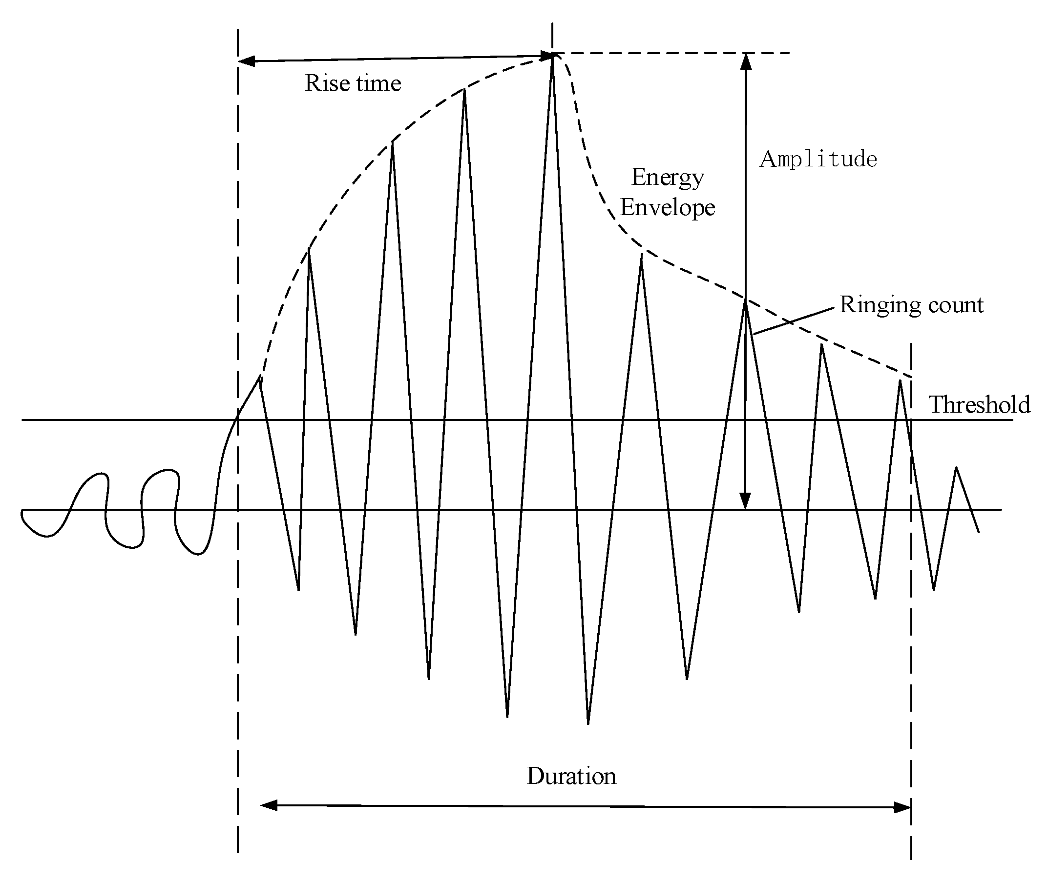
2.1.2. Waveform and Parameters of Acoustic Emission Signal

The AE signal is a non-smooth signal, which can be divided into burst type and continuous type [22]. Not only due to the complexity of the AE waveform signal collected in the actual bridge environment, but also considering the existence of reflection, refraction, and mode transformation during transmission, the received signal differs from the actual signal. In addition, it is difficult to describe the original AE signal accurately. Currently, the common method to describe the AE signal includes using the characteristic parameters of AE in the simplified waveform to describe the AE signal [23]. A simplified diagram of the AE signal is shown in Figure 1.

According to the simplified waveform of the AE signal, the main characteristic parameters include amplitude, duration, energy, rise time, ringing count, average signal level, event and threshold. The energy of AE signal is the area under the energy envelope, with the unit of ms*mV [23].

2.1.3. Acoustic Emission Signal Analysis Methods

The AE analysis methods applied in this paper include characteristic parameter correlation analysis, spectral analysis and wavelet analysis, respectively.

The purpose of the characteristic parameter correlation analysis method is to correlate two or more characteristic parameters to find out the influence of the correlation between the parameters [24]. Then, it further determines the nature of the AE signal through the influence relationship.

The AE signal is transient and random, and belongs to the category of non-smooth random signal. It consists of a series of frequency and mode rich signals. However, the signal characteristics in the time domain are rather one-sided for describing AE signal, since the transient signal is also accompanied by frequency and phase information. This requires further analysis of the signal in the frequency domain, i.e., spectral analysis. The spectral analysis method is to transfer the AE signal from the time domain to the frequency domain, and obtain the AE signal characteristics, as well as the state of the AE source through the time domain expression [25]. The most commonly used spectral analysis method for AE signals is the fast Fourier transform (FFT) spectral analysis method. The FFT method is a fast algorithm of discrete Fourier transform (DFT), which makes up for the shortcomings of the Fourier transform method in terms of operational efficiency. It has an important role in AE signal processing.

Wavelet transform (WT) is an effective mathematical tool [26]. The wavelet refers to its attenuation and fluctuation characteristics, respectively. It can show good local characteristics, since wavelets can have high resolution in time and frequency domains. The wavelet transform is also called a “mathematical microscope” by researchers because of its high resolution and the ability to focus on arbitrary details of the signal through the telescoping transform. The wavelet transform has been widely used in many fields, and has made outstanding contributions to the further characterization of AE signals.

The expressions of wavelet transform are shown in Equations (1) and (2).

$$W_f(a,b)={\displaystyle \underset{-\infty }{\overset{\infty }{\int }}f(t)\overline{{\phi }_{a,b}(t)dt}}$$

(1)

$${\phi }_{a,b}(t)=\frac{1}{\sqrt{a}}\phi (\frac{t-b}{a})$$

(2)

In the above equation, $a$ is the scale factor, $b$ is the translation parameter and $\phi (t)$ is the wavelet. According to the mathematical expression of the wavelet transform, it transforms the time function to the time-scale plane and focuses on the details of the time-domain function by the scale factor and the translation parameter. This makes it possible to extract certain features of the mutated signal.

The choice of wavelet basis is also an important issue of the wavelet transform. The wavelet basis functions include Harr wavelets, symlets, Daubechies wavelets, Meyer wavelets, and Coifman wavelets, etc. The selection of wavelet basis functions is related to the correctness and validity of the analysis results. The Daubecheies (db) wavelet is a finite tightly-branched orthogonal wavelet with a long enough support width, and the vanishing moment and regularity are also superior. According to the wavelet analysis of the AE signal, the number of decomposition layers should not exceed five layers [27].

2.2. Acoustic Emission Signal Segmentation Algorithm

The common AE signal is a burst signal. However, when we carry out signal acquisition, the signals collected by the acquisition card are continuous. How to find the burst signal from the continuous signal, and how to determine the start point and end point of the burst signal are the problems that need to be solved. Inaccurate judgment of the start and end points of the AE signal may lead to inaccuracy of the characteristic parameters. The calculation of parameters such as energy, ringing count and duration of the AE signal is related to the length of the AE signal. Moreover, using the proposed algorithm to segment the signal may save effort and be more time efficient compared with manual segmentation. The acquisition card used in the experiments of this paper is a general-purpose acquisition card for AE signals. This kind of acquisition card can only acquire AE signals continuously, but does not have the function of segmenting the AE signals and calculating the subsequent characteristic parameters. Therefore, it is indispensable for the subsequent analysis of the AE signal to accurately segment an AE signal from the acquired continuous waveform stream. In this paper, we propose an AE signal segmentation algorithm using the characteristics of AE signal. This proposed pre-processing algorithm has great significance for the future AE signal identification in the health monitoring system for bridge cables.

In general, the AE signal is segmented from the acquired continuous waveform, mainly to find the start and end points of the AE signal. The algorithm segments the signal based on the following parameter values and the specific meaning of each parameter is shown below:

• Threshold (Thr):

When we analyze the continuous waveform acquired from the acquisition card, the part of the signal without AE signals needs to be filtered out. We may set a value as the threshold. If the amplitude of the collected signal in the data stream has not exceeded the set threshold, it may be filtered out. When the amplitude of an existing signal crosses the threshold, it is considered the arrival of an impact signal. The time when the point exceeds Thr is the start time of the AE signal.

• Hit Definition Time (HDT):

After starting to segment the AE signal, finding the end point of the AE signal is the next step to be carried out. When the amplitude of the acquired AE signal changes from higher than Thr to lower than this value, the HDT timer is triggered. If the amplitude of AE signal remains lower than Thr within HDT, the last point that crosses the threshold is considered to be the end point of the AE frame. Then, the process of segmenting the signal is also finished after the judgment. The next section of signal reading and judgment is carried out.

• Hit Lockout Time (HLT):

For some AE signals, a subsequent rebound wave may exist. In order to avoid misjudging the rebound wave of the AE signal for the next AE signal waveform, the parameter of hit lockout time (HLT) is introduced. After obtaining a frame of AE signal, regardless of whether there is a signal that exceeds the threshold or not, the signal from the acquisition card within the period of HLT will be ignored. It will not trigger the HDT judgment mechanism either.

• Maximum Duration (MD):

At some special moments, AE signals may be too dense to be distinguished separately. If the amplitude of the signal remains higher than Thr, the parameters mentioned above may not effectively segment the AE signal. To resolve this problem, we introduce the parameter maximum duration (MD). When the signal length exceeds MD, the acquired signal is mandatorily segmented. From the start time to the time when the signal exceeds MD, its frame is treated as a complete AE signal.

By setting the above basic parameters, the flow of the algorithm is designed as shown in Figure 2.

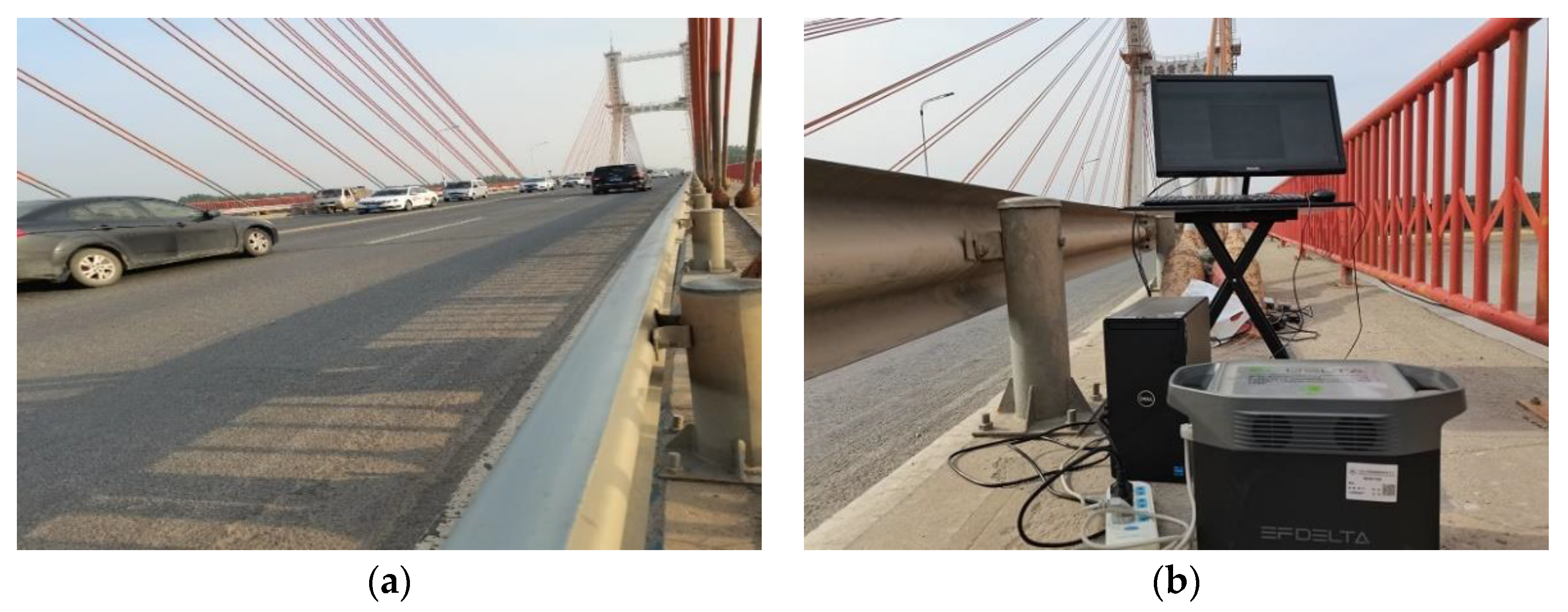
2.3. Noise Signal Acquisition Experiment

In the application of health monitoring of bridge cables, we attach AE sensors on the bridge cables to acquire signals. Under the real environments on bridges, the noise may have a great impact on the AE signal acquisition. Previous research might study the noise characteristics by simulation [6,7], or treat the noise as simple white noise model [8]. Some researchers conducted AE experiments in the laboratory and ignored the existing noise under real environments [9,10]. In order to study the noise characteristics under real environments, signal acquisition experiments were conducted on three bridges, namely Yantai Yangma Island Bridge, Jinan Yellow River Bridge and Shenzhen Caihong Bridge. All three bridges are either boom or cable-stayed bridges. The experiments were conducted under normal bridge operation in order to obtain the noise signals when monitoring the bridge health using AE technology. In the experiments, we use Spectrum’s high-speed acquisition card, M2p.5922-x4. Its acquisition resolution is 16 bit and its acquisition rate is 3 MS/s. The sensors selected for this experiment are SR40M and SR150M, with acquisition frequency bandwidths of 15~70 kHz and 60~400 kHz.

The experimental site plan for signal acquisition in the field test is shown in Figure 3, Figure 4 and Figure 5.

3. Results

3.1. Segmentation Algorithm Results

A continuously acquired signal was analyzed to verify the proposed AE signal segmentation algorithm. The AE segmentation parameters were set as follows: threshold Thr is 0.1 V, HDT is 0.002 s, HLT is 0.002 s, and MD is 1 s. The waveform data stream acquired before segmentation is shown in Figure 6.

The segmented signals are shown in Figure 7a–e. There are five AE signals above 0.1 V in this continuous waveform. The signal occupies 2.01 GB of memory space before segmentation and 52.6 MB in total for the five segments after segmentation. This proposed segmentation algorithm saves 97.5% of memory space while facilitating the extraction of the signal feature parameters.

3.2. Feature Parameter Extraction

The calculation program for the characteristic parameters is written in MATLAB to realize the segmentation waveform and calculation of the characteristic parameters. The main parameters include rise time, duration, ringing count, amplitude, energy, average frequency, and average signal level characteristics. Due to the low amplitude of the noise signal, the calculation threshold of the AE parameters is chosen.

Since this experiment has a 20 dB preamplifier, it is 45 dB after conversion according to Equation (3). Considering that the noise is a continuous waveform with a longer duration compared to the burst AE signal waveform, the segmentation parameters set for the segmentation noise are HDT = 0.02 s, HLT = 0.2 s, and MD = 3 s.

$$\mathrm{dB}=20\lg \frac{U}{1 \mathsf{\mu }\mathrm{V}}$$

(3)

where 1 µV is 0 dB and U is the maximum voltage value.

A total of 619 noise signals were acquired from Yangma Island Bridge, 3440 noise signals were collected from Yellow River Bridge, and 1552 noise signals were collected from Shenzhen Caihong Bridge. We randomly selected 100 among them to present their calculated characteristic parameters, as shown in

Table 1. Noise signal characteristics parameters table.

Serial Number	Rise Time (µs)	Duration (µs)	Ringing Count	Amplitude (dB)	Energy (ms*mV)	AF (kHz)	ASL dB
1	11,949	12,396	13	53	2.86	1.05	28
2	199	42,193	375	61	76.53	9.68	24
3	3977	46,368	449	62	90.60	10.87	25
4	1442	50,859	553	58	59.76	8.58	22
5	1425	46,252	397	59	58.15	8.02	23
6	628	44,164	354	60	62.19	13.58	24
7	151	38,947	529	62	91.63	12.43	26
8	3514	48,656	605	62	91.85	14.43	26
9	5220	44,630	644	60	100.40	12.75	26
10	1228	48,475	618	61	76.53	15.64	26
11	4376	13,906	42	54	11.91	3.02	19
				……
90	967	17,304	222	53	23.01	13.59	39
91	633	834	20	49	27.49	15.92	27
92	4070	27,566	122	53	23.74	4.43	19
93	12,087	38,825	436	56	53.22	11.23	23
94	34	4632	33	52	4.97	7.12	21
95	2051	16,362	321	58	30.35	19.62	25
96	1537	12,592	171	58	22.20	13.58	25
97	2147	9154	85	53	10.77	9.29	22
98	4661	19,550	180	60	33.56	9.21	25
99	4048	13,517	178	54	20.40	13.17	20
100	3007	34,021	351	65	114.52	10.32	30

. The subsequent analysis is performed according to the calculated noise signal characteristics.

3.3. Comprehensive Noise Analysis

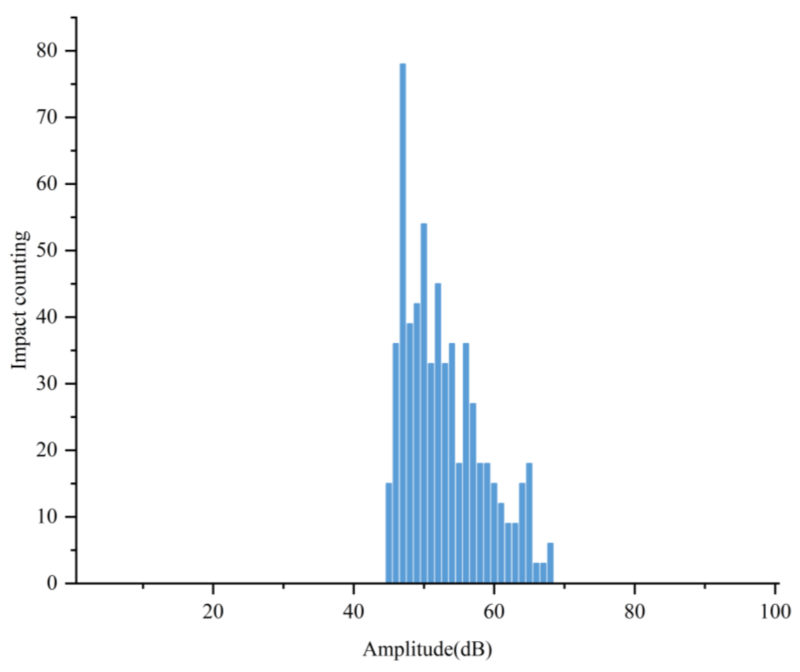
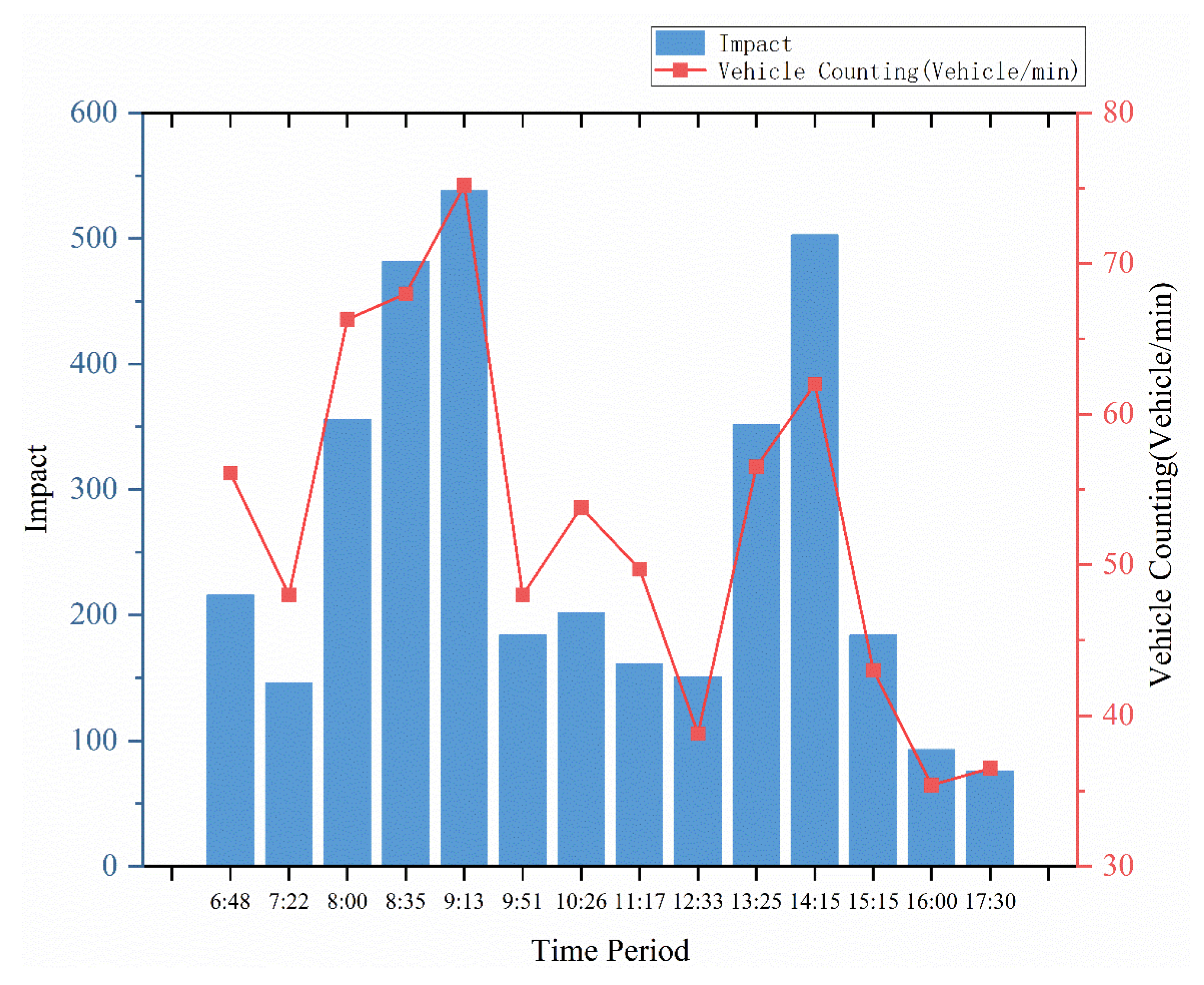
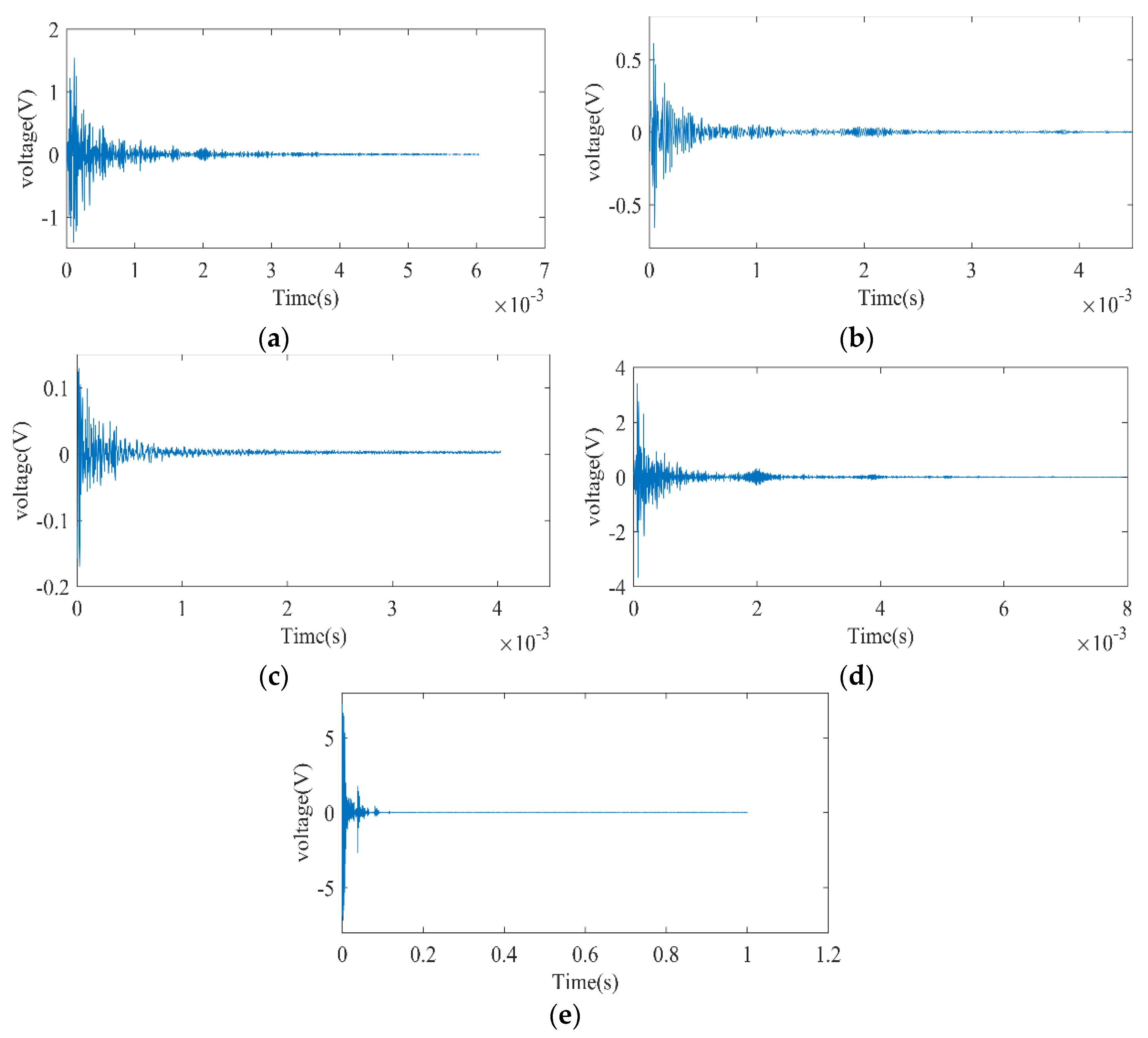
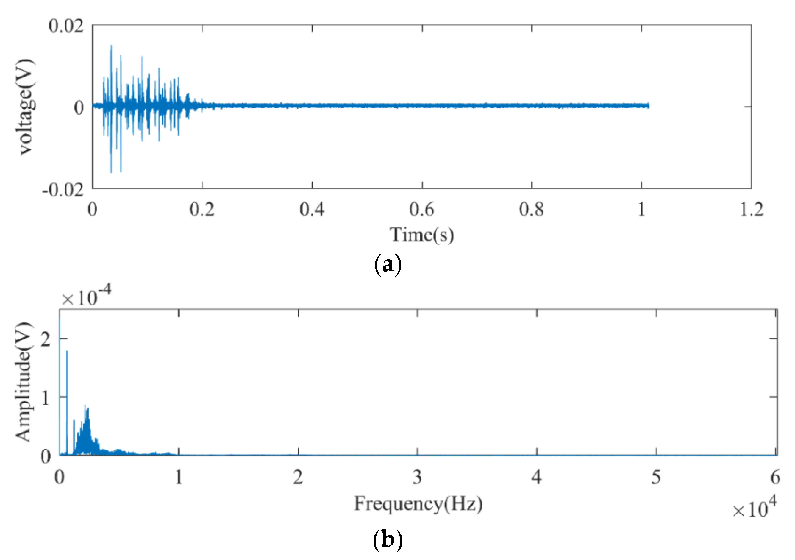
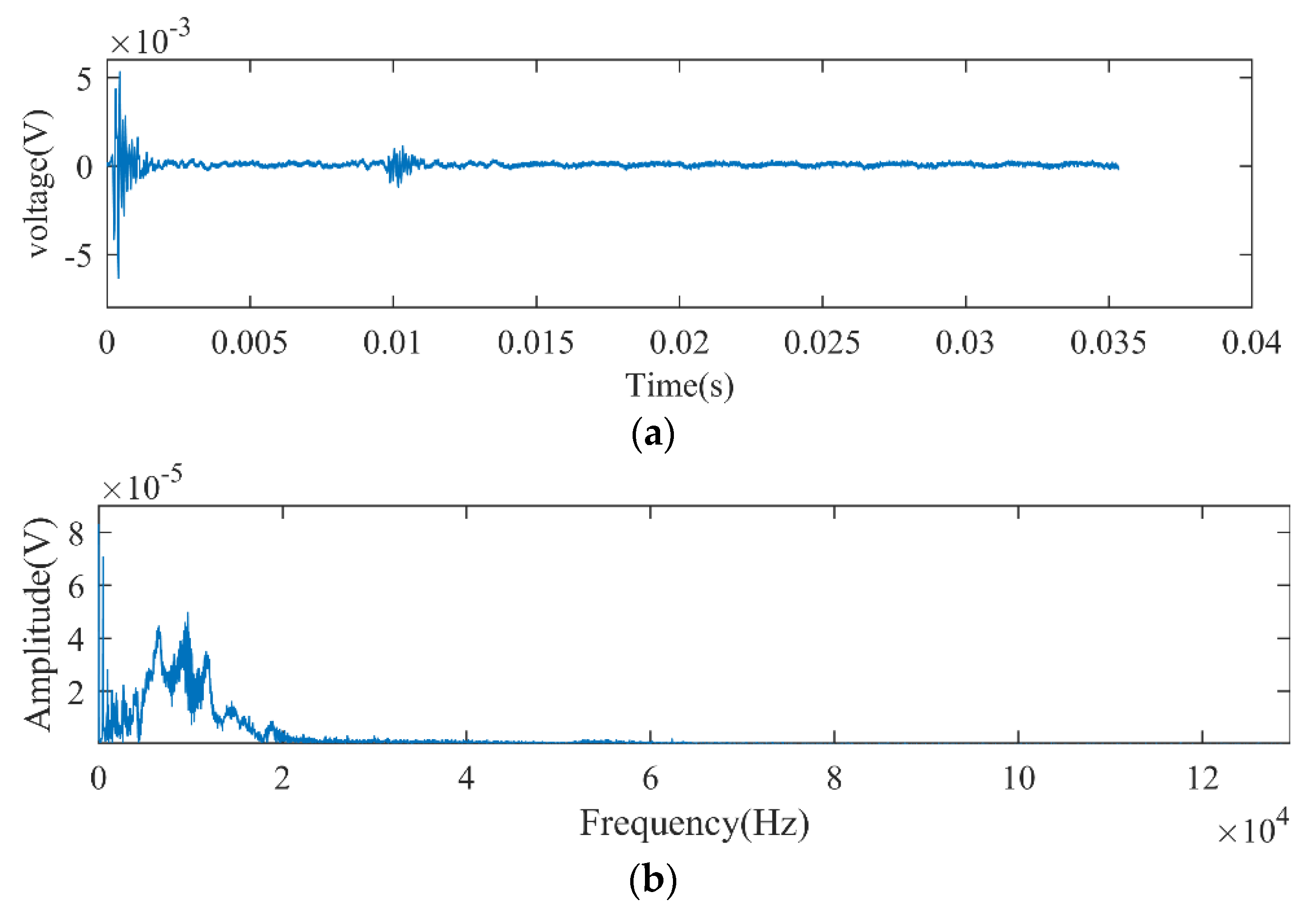
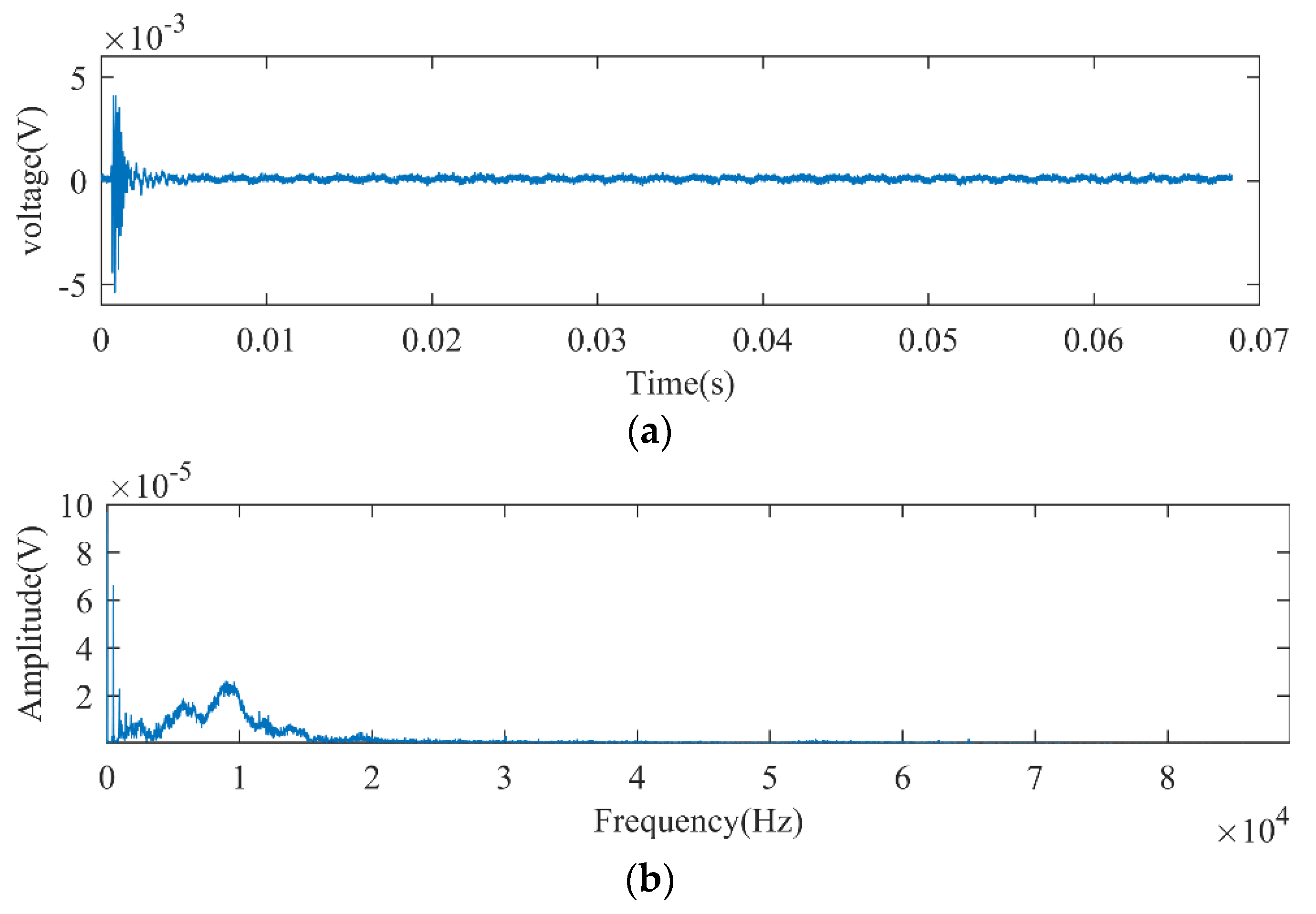
3.3.1. Time Domain Analysis

The following analysis of the noise signal was carried out in the time domain:

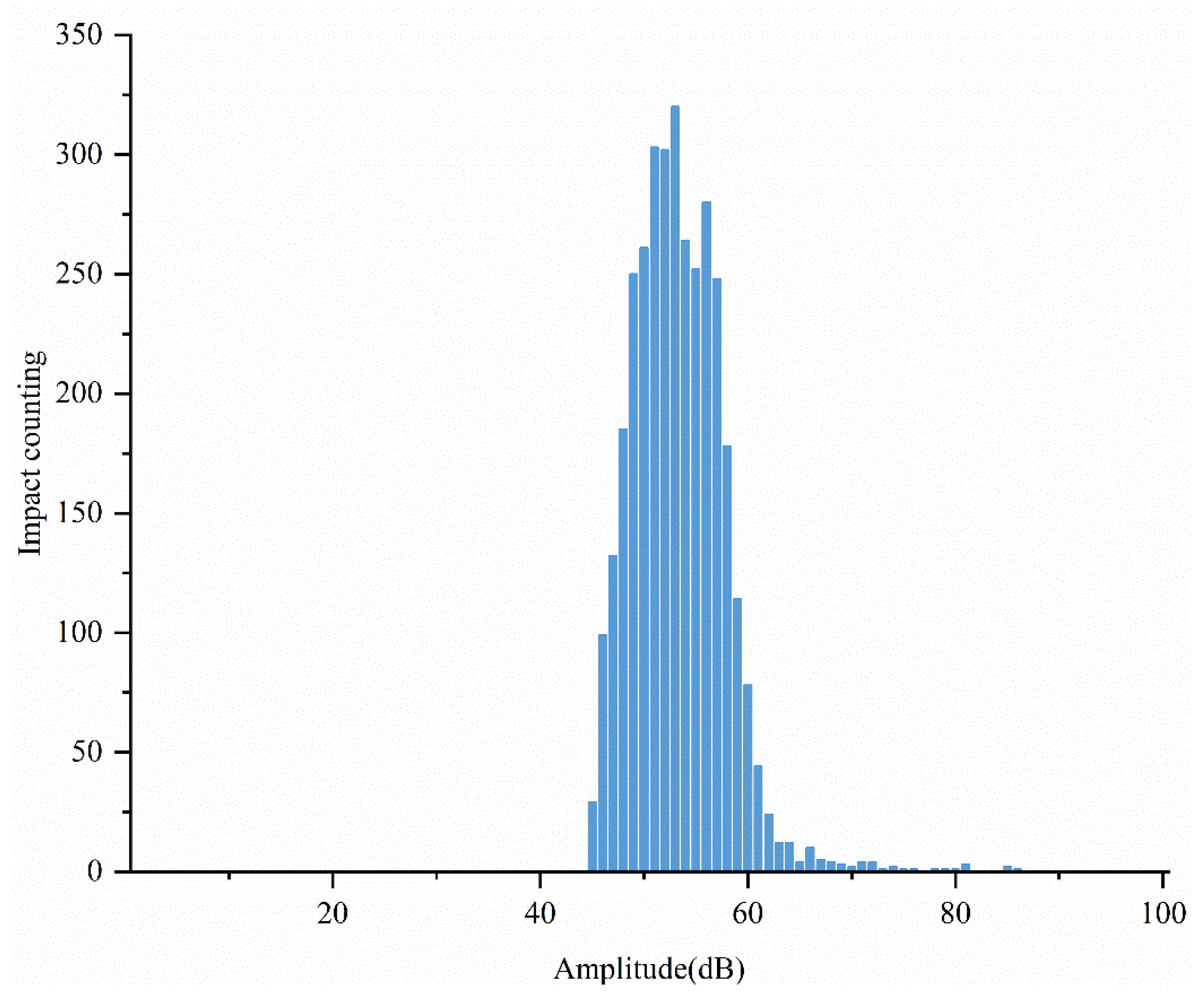
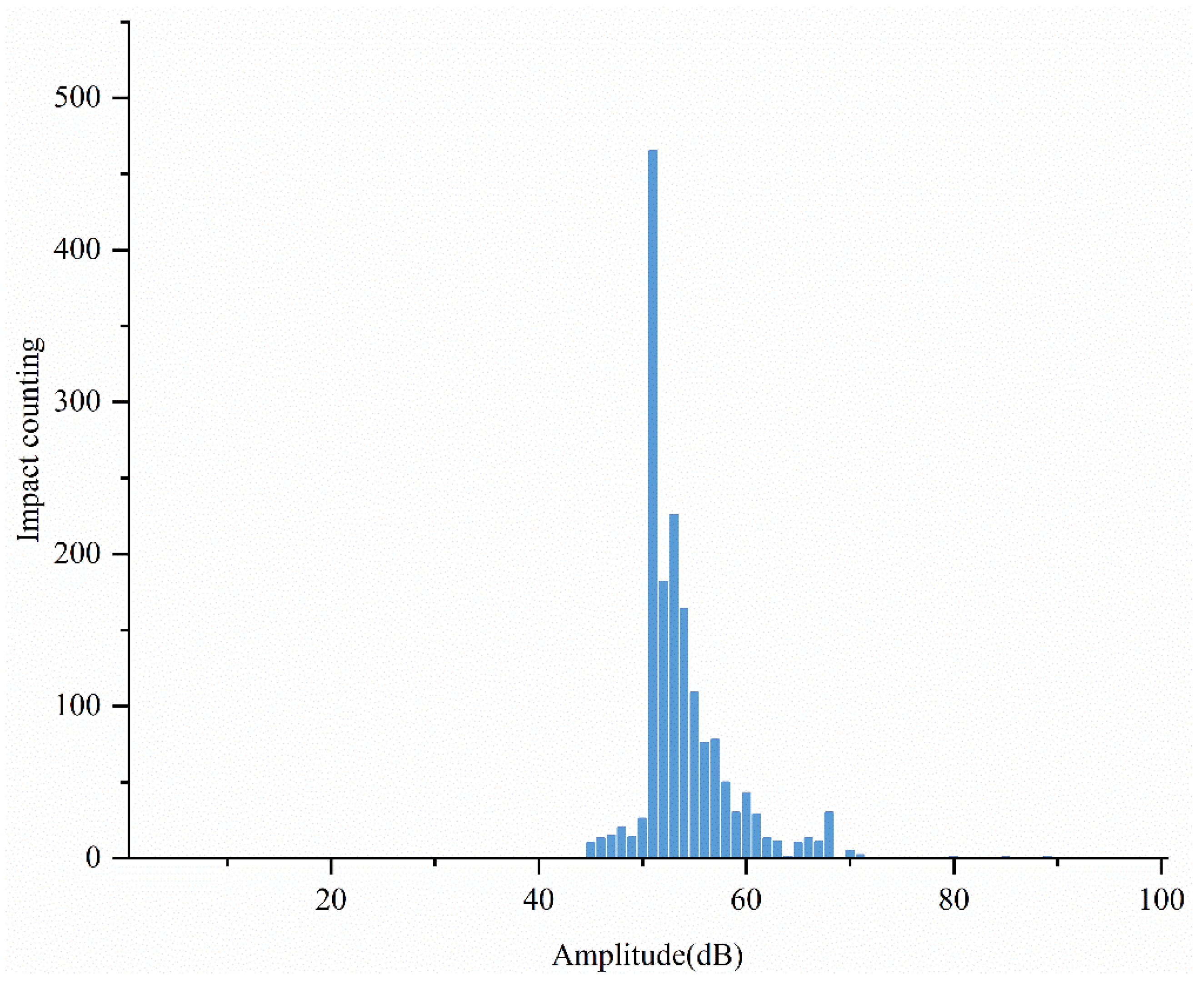
• Impact-amplitude correlation analysis;

Unlike the ringing count of a signal, when an AE signal waveform reaches its maximum value, an impact is formed at that value. Through the impact-amplitude correlation analysis, the distribution interval of the collected noise amplitude can be derived.

The impact-amplitude correlation plots of the noise signals of the three bridges are shown in Figure 8, Figure 9 and Figure 10.

The impact count amplitude of the noise signal collected from each bridge is normally correlated, with few high and low amplitude signals. The amplitudes of noise at each bridge mainly concentrate between 50 dB and 70 dB. We notice that the noise signal at 80 dB of Yangma Island Bridge did not cause impact and few impacts occurred with the noise between 80 dB and 90 dB at the other two bridges. Therefore, according to the distribution of the impact-amplitude correlation diagrams of the three bridges, the threshold for filtering noise can be set at 80 dB. Then, most of the noise can be filtered out by segmentation analysis after 80 dB.

2.

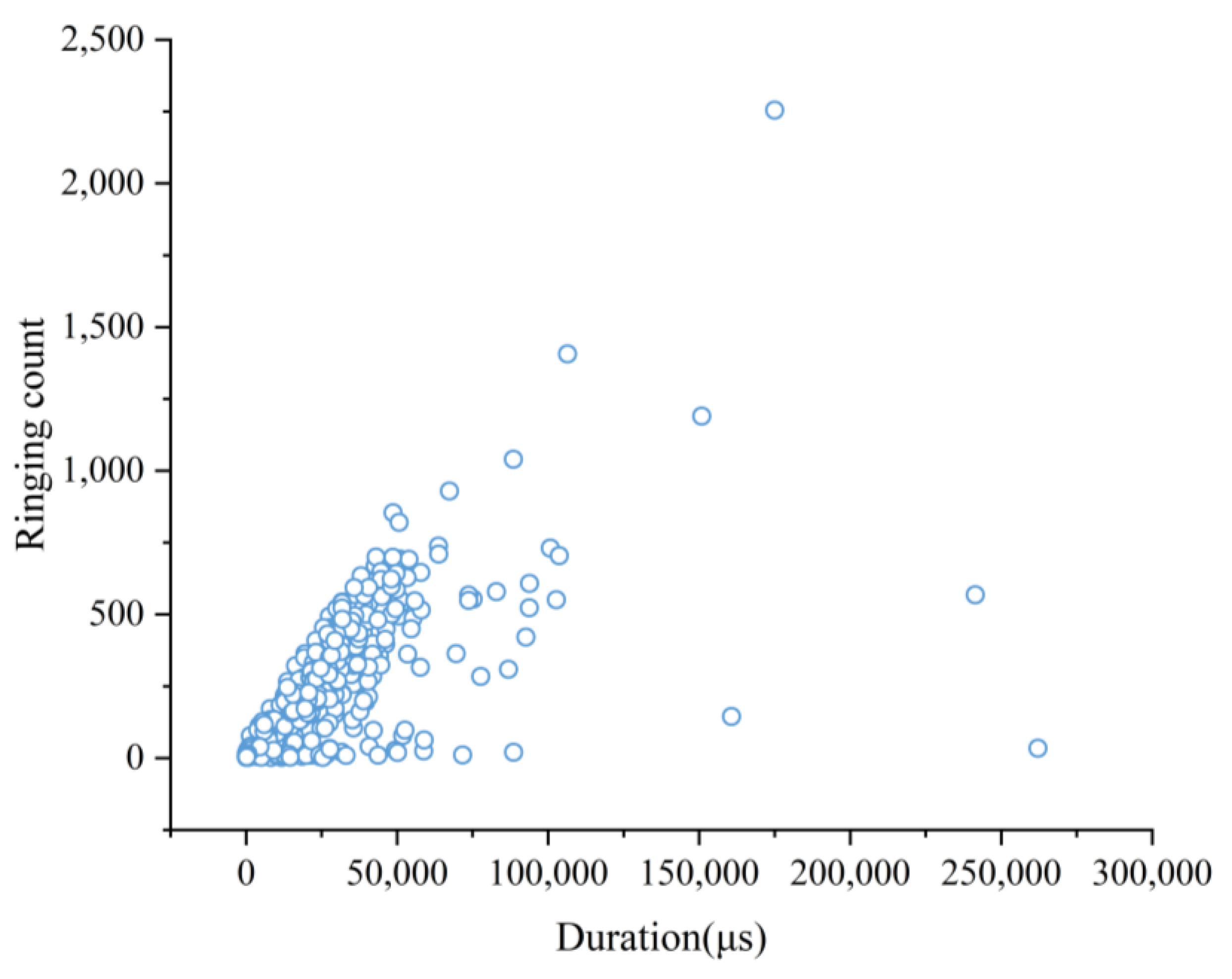
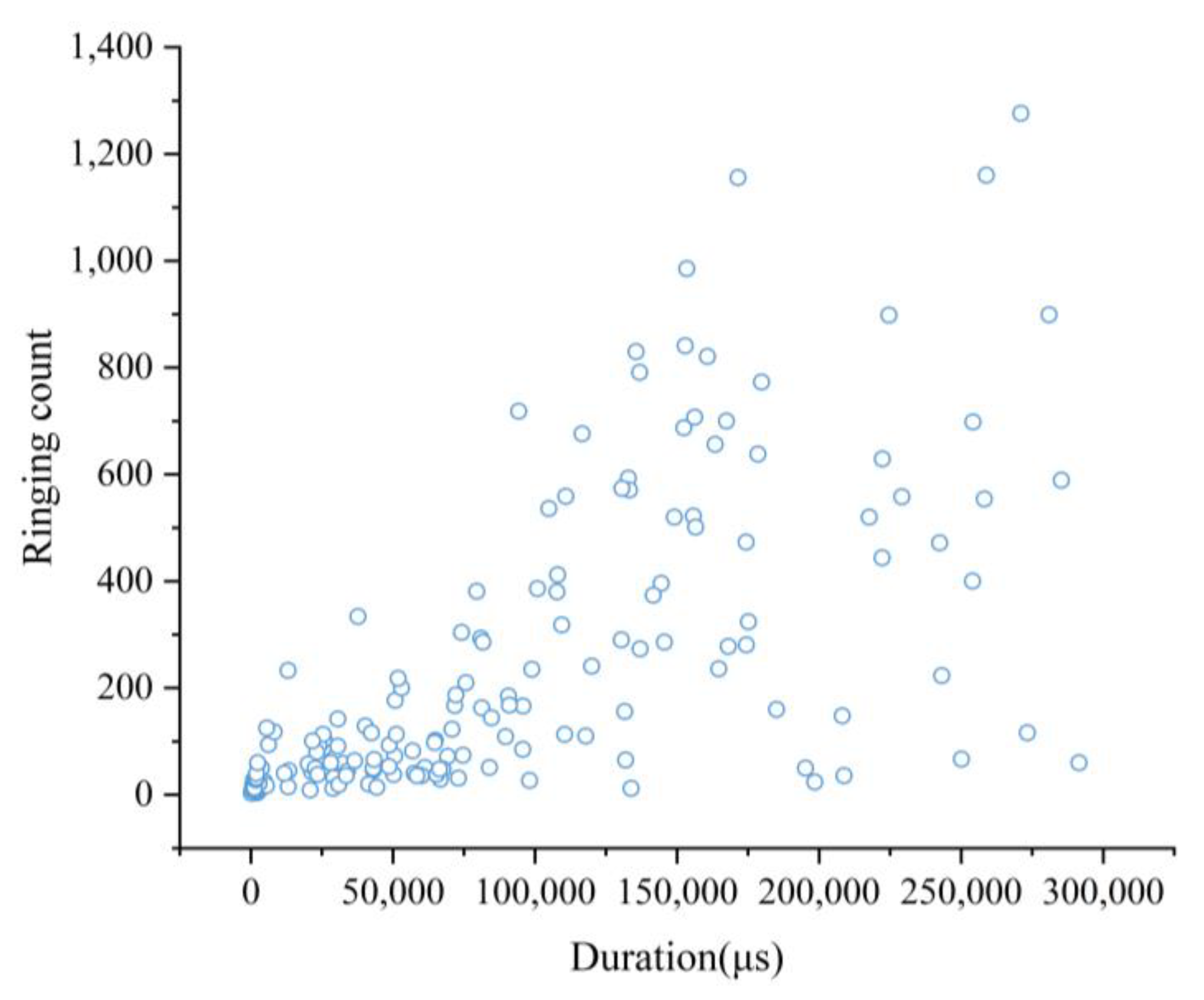
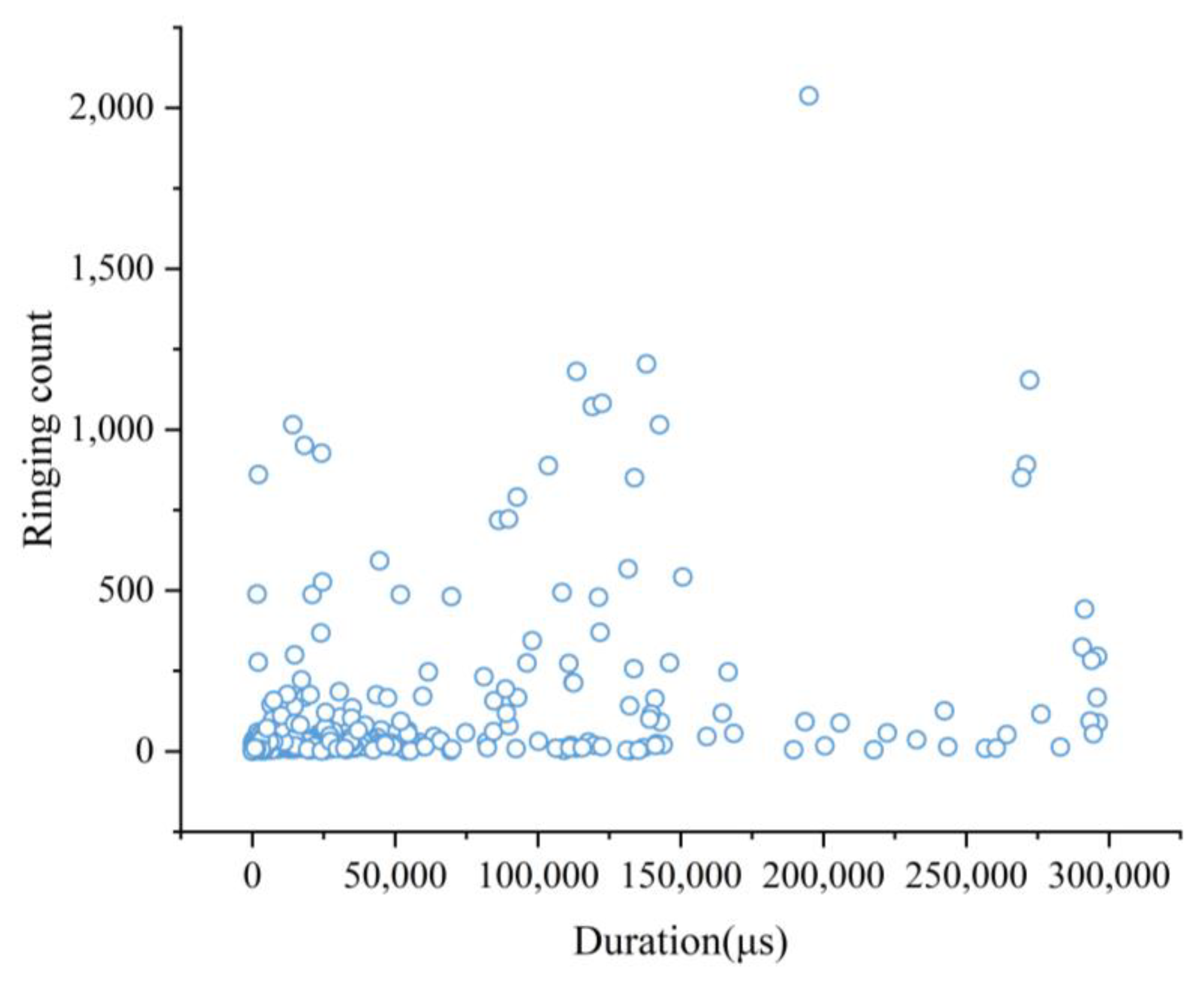
Ringing count-duration correlation analysis;

Although the amplitude is the main reference parameter for signal filtering, there may still exist cases where the signal amplitude is high but the ringing count or duration is short. Thus, other characteristic parameters are needed as the basis for filtering the noise signal. The ringing count reflects the number of pulses above the analysis threshold (45 dB) of a noise signal, representing the intensity and frequency of the noise signal. A high ringing count within a short duration indicates that the signal energy release is concentrated. The correlation analysis of the two characteristic parameters can provide a reference to the noise filtering in the time domain, and the noise signal with high energy in a short time can be filtered out by setting the appropriate time parameters. Figure 11, Figure 12 and Figure 13 depict the noise signal duration and ringing count correlation analysis for the three bridges.

From the ring count-duration correlation diagram of the noise signals of the three bridges, it can be observed that there is an obvious positive correlation between the magnitude of the ringing count and the duration, except for the fact that the noise signal is the least obvious at Yellow River Bridge. The duration and ringing counts of the noise signals collected at the three bridges are relatively small, and the noise signals generally complete the ringing counts within 0.15 s, i.e., the main energy of the signal can be released within that time. Therefore, the duration of 0.15 s and the 1000 ringing counts can be used as the threshold indicators for filtering noise signals. Signals smaller than this duration and ringing counts can be identified as noise.

3.

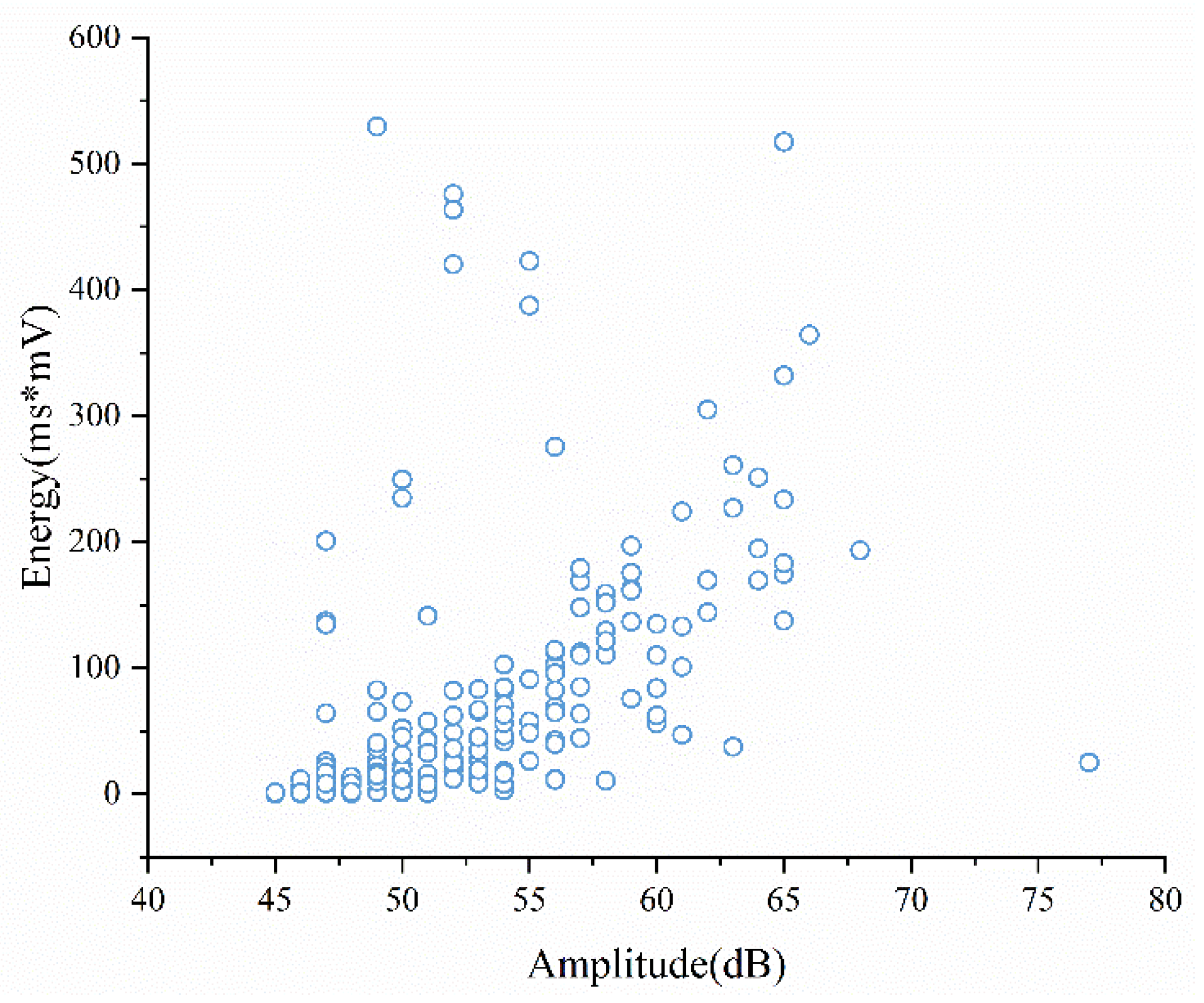
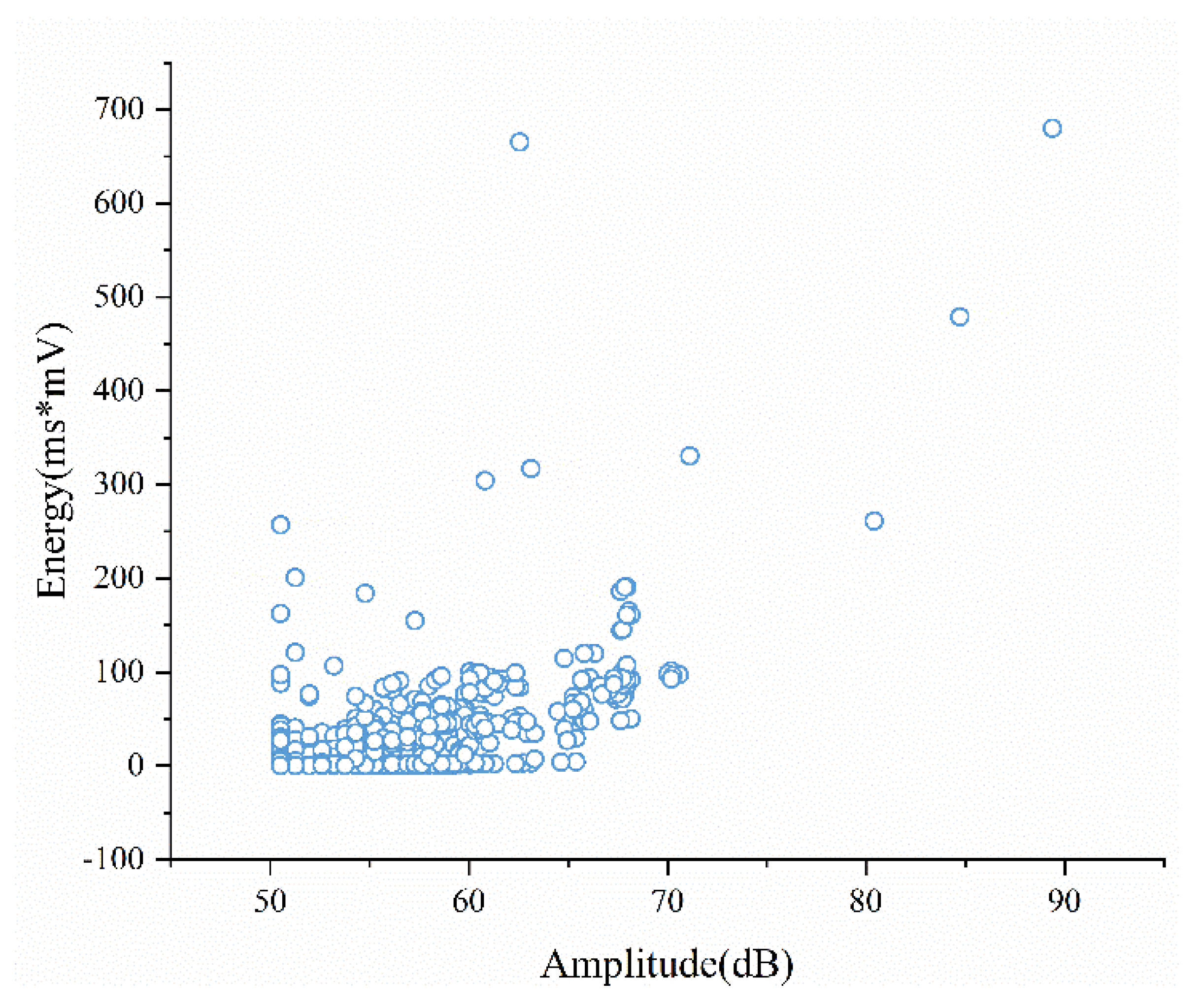
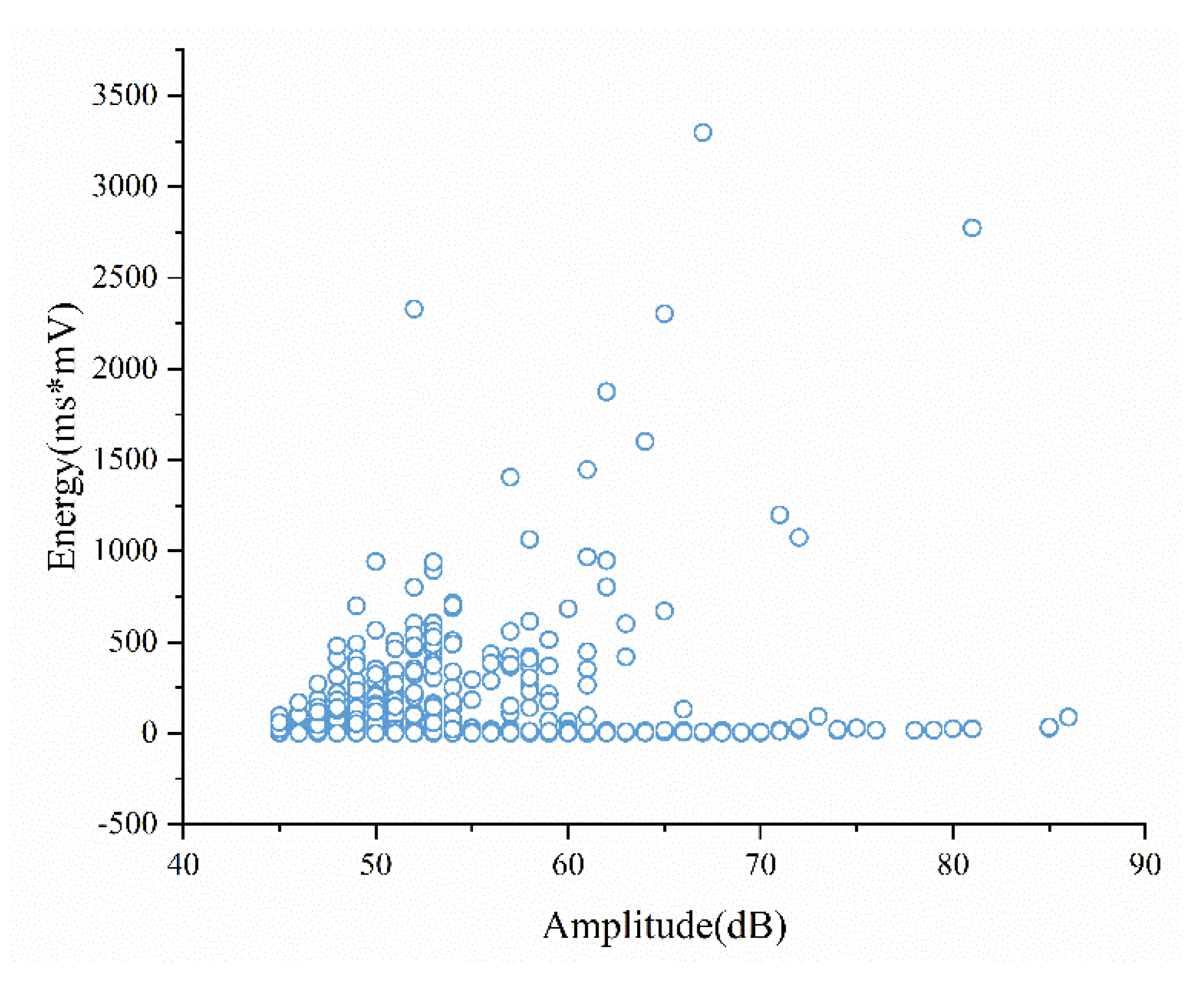
Amplitude-energy correlation analysis;

Figure 14, Figure 15 and Figure 16 depict the amplitude-energy correlation analysis of the noise signals of the three bridges. The intensity of the AE source is directly related to the magnitude of the AE signal. The correlation analysis of energy and magnitude is one of the methods to reflect the information of the AE source. In order to avoid the noise signal with high amplitude being analyzed later or being mistaken for the cable break signal, the reference of the energy characteristic parameter is added.

The experimental results show there is a positive correlation between amplitude and energy, and the noise of Yangma Island Bridge is the most obvious. The noise signals collected at the three bridges are mostly low-energy signals within 1000 ms*mV. The signal amplitudes of Yangma Island Bridge and Rainbow Bridge are lower, within 600 ms*mV and 700 ms*mV. The signal amplitudes within 1000 ms*mV of Yellow River Bridge also account for more than 99%. The signal amplitude of Yellow River Bridge within 1000 ms*mV also accounts for more than 99%. Thus, the energy parameter of 1000 ms*mV can be used as a threshold indicator to identify noise. The noise signal of Yellow River Bridge is higher in energy with the same amplitude, which is related to the intensive traffic flow of Yellow River Bridge during the experimental process.

4.

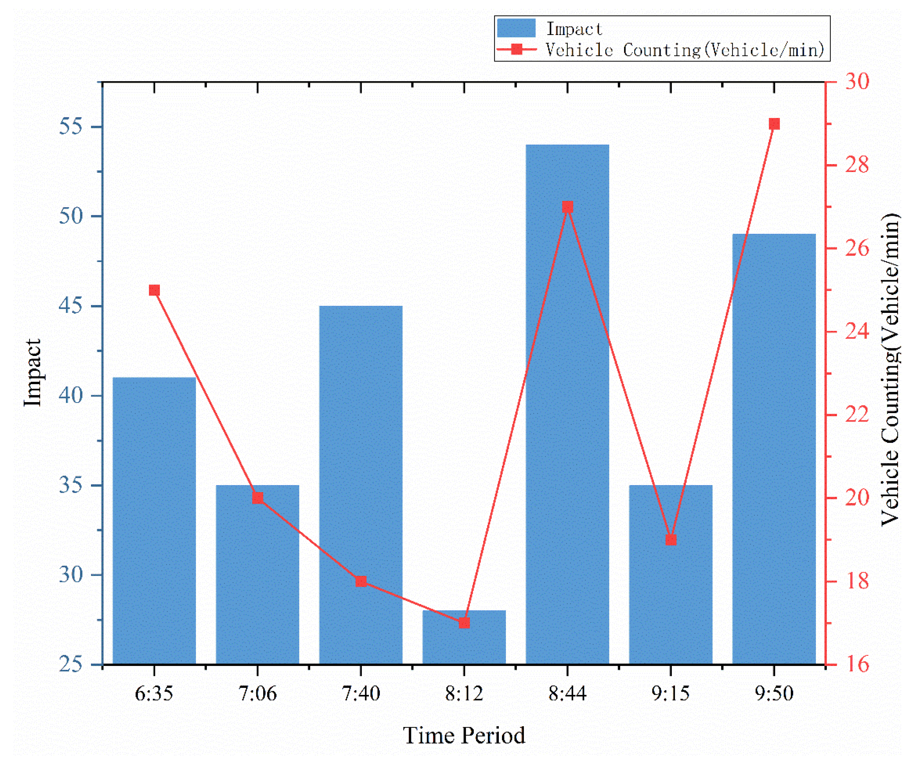
Impact-vehicle count correlation analysis;

Figure 17 and Figure 18 show the noise signal impact-vehicle count correlation plots at locations 1 and 2 of Yellow River Bridge. During the AE signal acquisition experiments at Yellow River Bridge, vehicle counts were conducted. Every 0.5 h was the period. Six vehicle counts with one-minute duration each were performed within that period. The average value of the six counts was used as the average vehicle count parameter value within that period. We can observe that there is an obvious linear relationship between vehicle counts and crash counts. The more vehicles pass by during that time period, the more noise signals with high amplitude will be generated and form more crash signals. It also indicates that the main source of noise signals is the vehicles driving by on the bridge. All other time periods are consistent with the linear relationship between the number of impacts and vehicle counts, except the time period starting from 7:06 at location 2. The noise signal at location 2 was collected at 7:00~9:00 when the traffic jam occurred in the morning traffic peak, and the number of vehicles driving through the collection point was low per unit time period. Therefore, the noise caused by the cars staying at the sampling point was not enough to cause the impact signal.

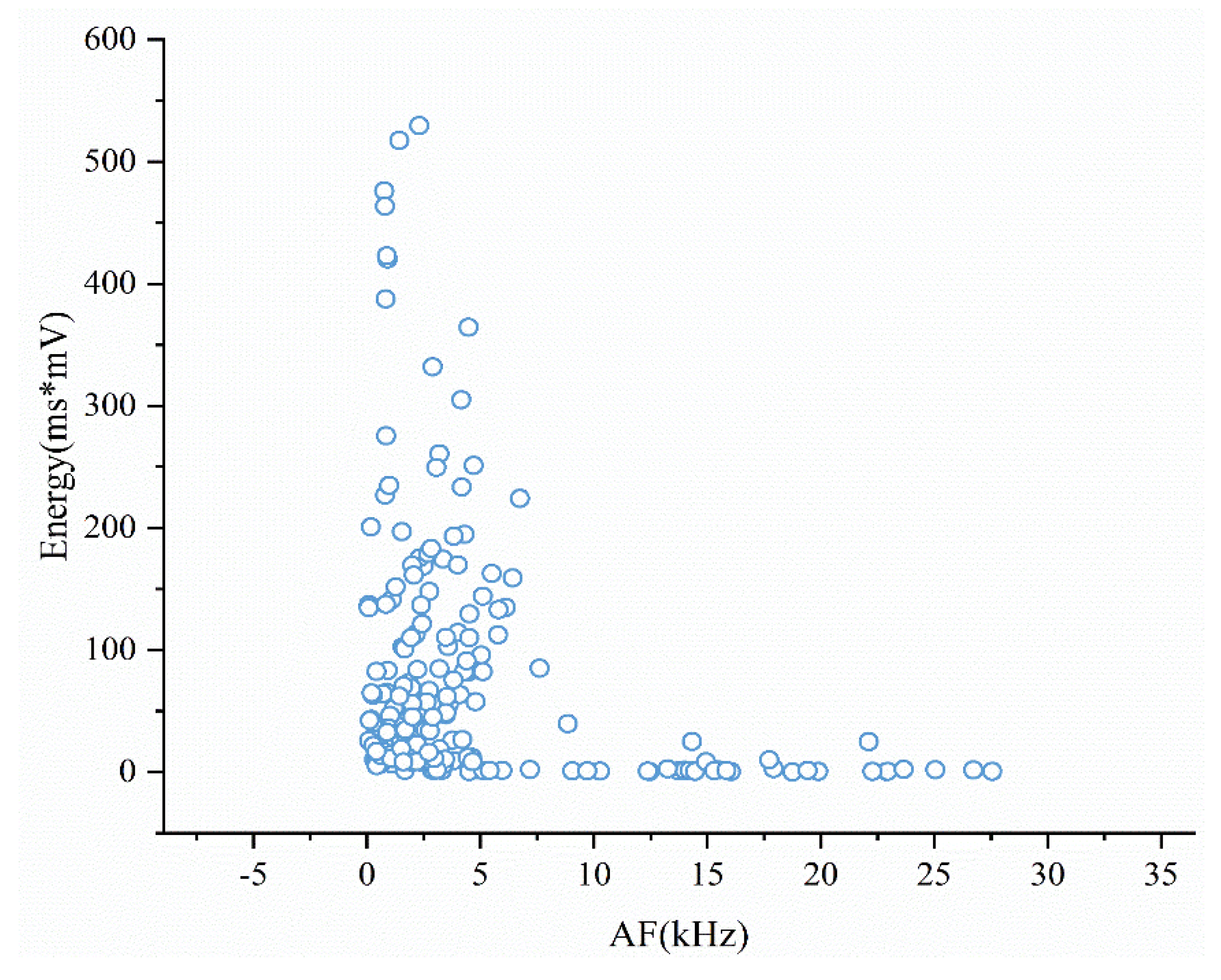
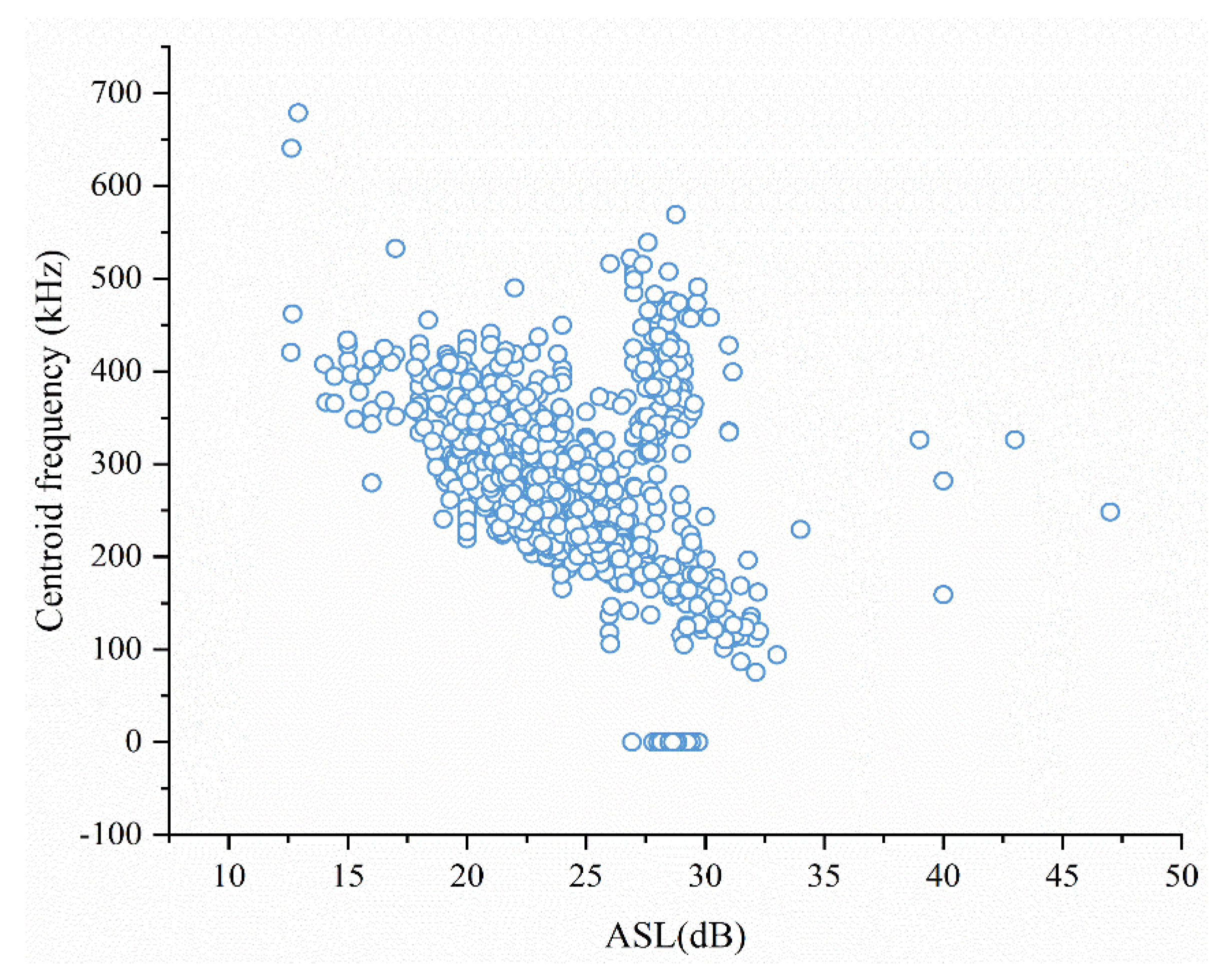
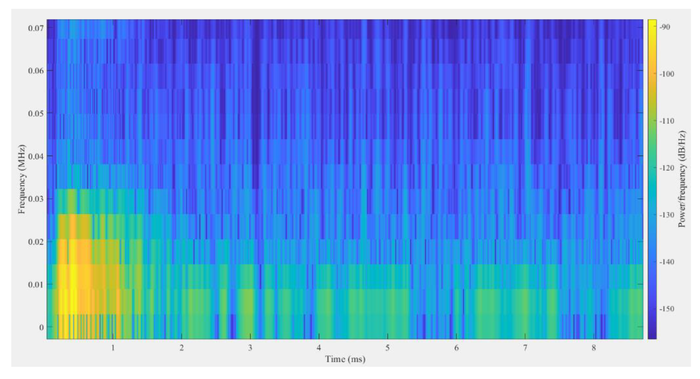
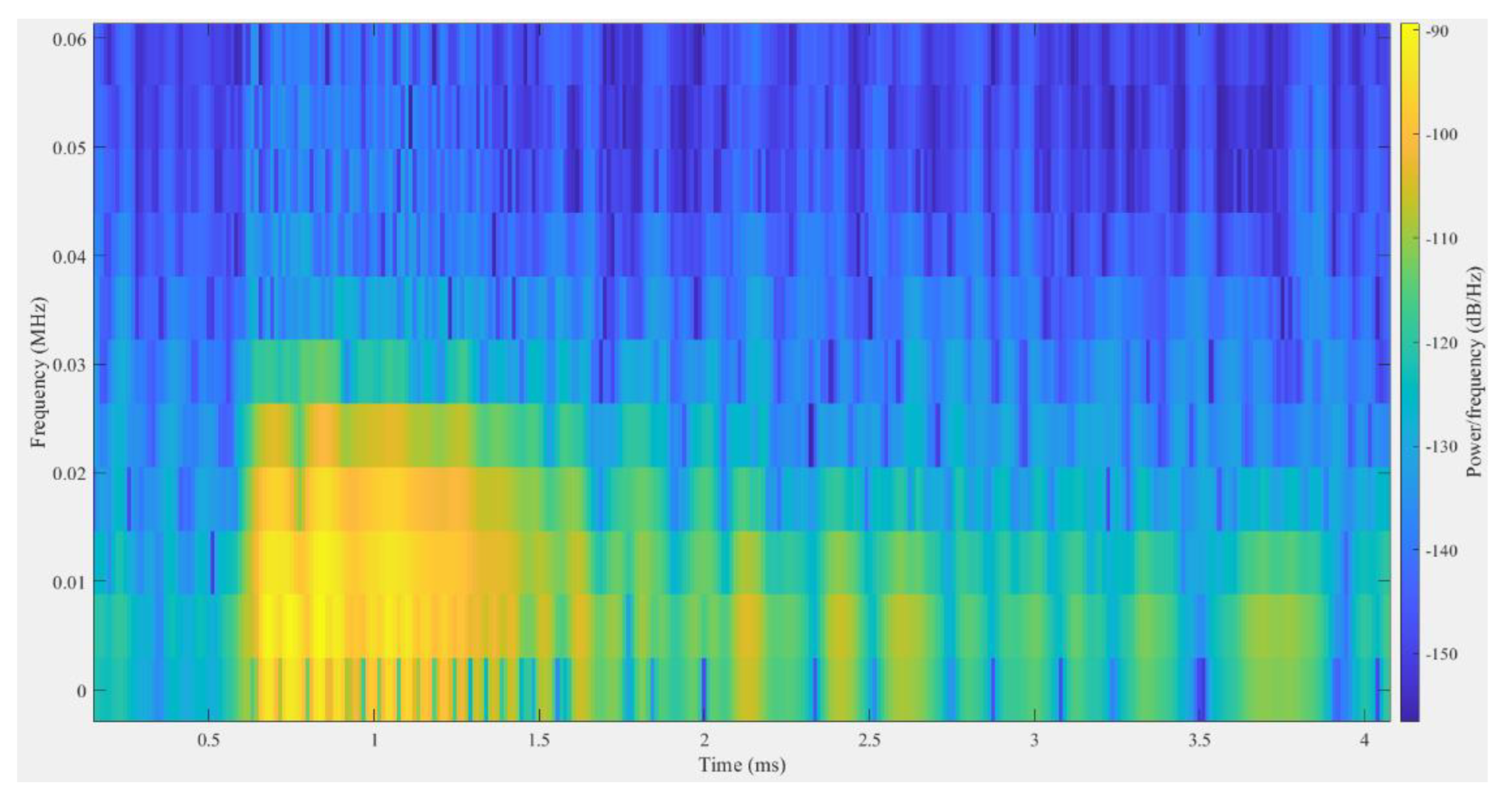
3.3.2. Frequency Domain Analysis

The following analysis of the noise signal is performed in the frequency domain:

• Signal spectrum analysis

The FFT method is used to transform the noise signal from the time domain to the frequency domain to obtain the characteristic distribution of the noise signal in the frequency domain. Nearly one hundred noise signals at each bridge cable were FFT transformed, and the representative noise signals of each bridge were selected randomly. The time and frequency domain plots of the signal are shown in Figure 19, Figure 20 and Figure 21.

From the above figures, we can learn that the spectral range of the noise signals of the three bridges are concentrated within 20 kHz.

2.

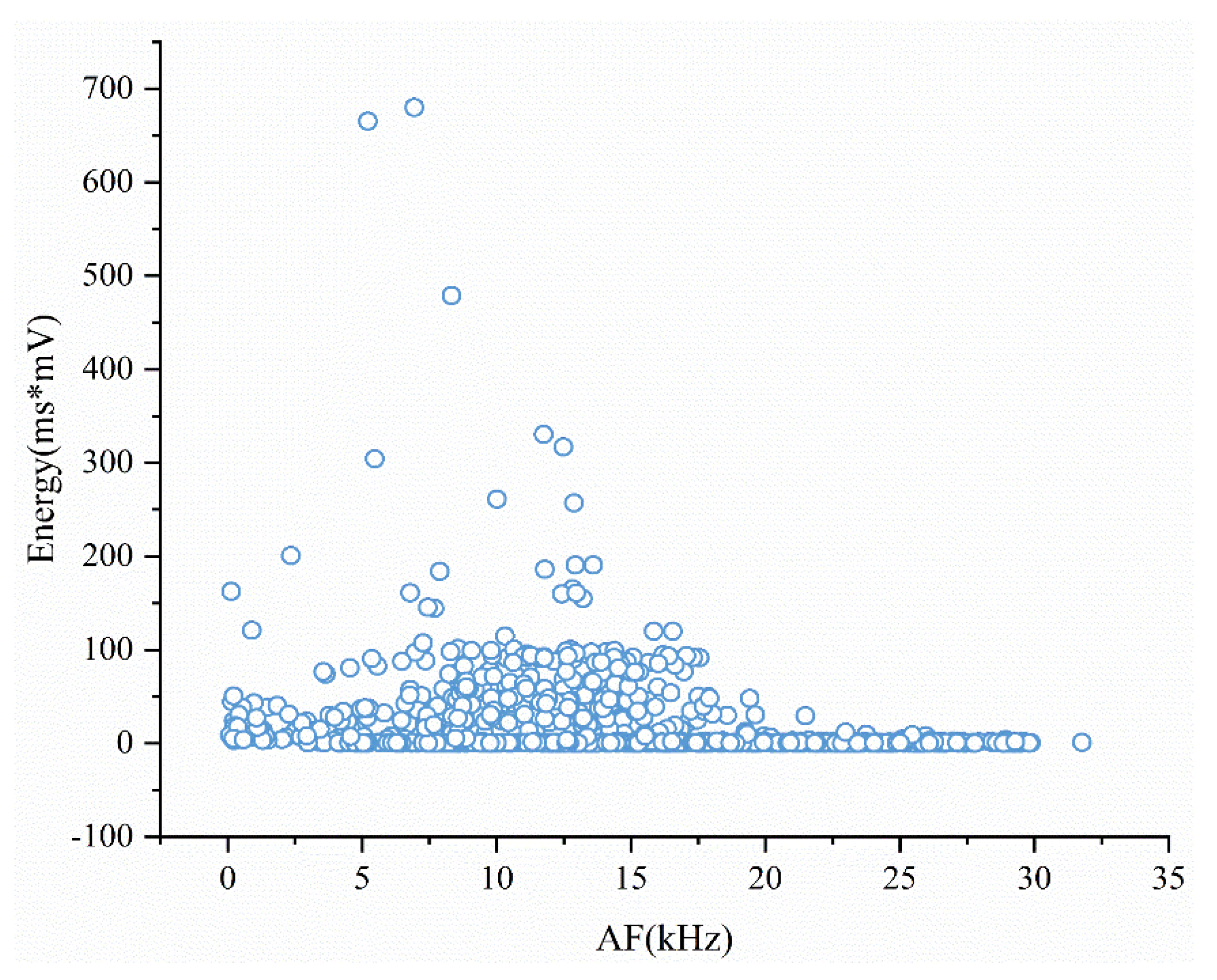
Energy-average frequency correlation analysis

Average frequency (AF) indicates the number of times the AE signal exceeds the threshold value. Thus, AF is defined as the ringing count divided by the duration. Compared with the AE signal of broken wires, the noise signal has a smaller ringing count and longer duration, i.e., smaller AF value. So, the AF value is an important discriminative parameter for the noise signal.

Figure 22, Figure 23 and Figure 24 illustrate the correlation analysis of the average frequency-energy of the noise signals of the three bridges.

From the above three average frequency-energy correlation plots, we find that the correlation between average frequency and energy is not obvious. This indicates that the activity of the AE source is relatively independent of the type of AE signal. The average frequency of high-energy noise signals is mainly concentrated in the range of 20 kHz. There are noise signals in the range of 20 kHz to 30 kHz, but the energy is low. The average frequency of the noise signal of Yangma Island Bridge is less than 20 kHz and has a proportion of 96.1%. The average frequency of the noise signal of Yellow River Bridge is also less than 20 kHz and has a proportion of 90.6%. The average frequency of the noise of Caihong Bridge is also less than 20 kHz and has a proportion of 91.7%. Therefore, the average frequency threshold of 20 kHz can filter out most of the high-energy noise signals.

3.

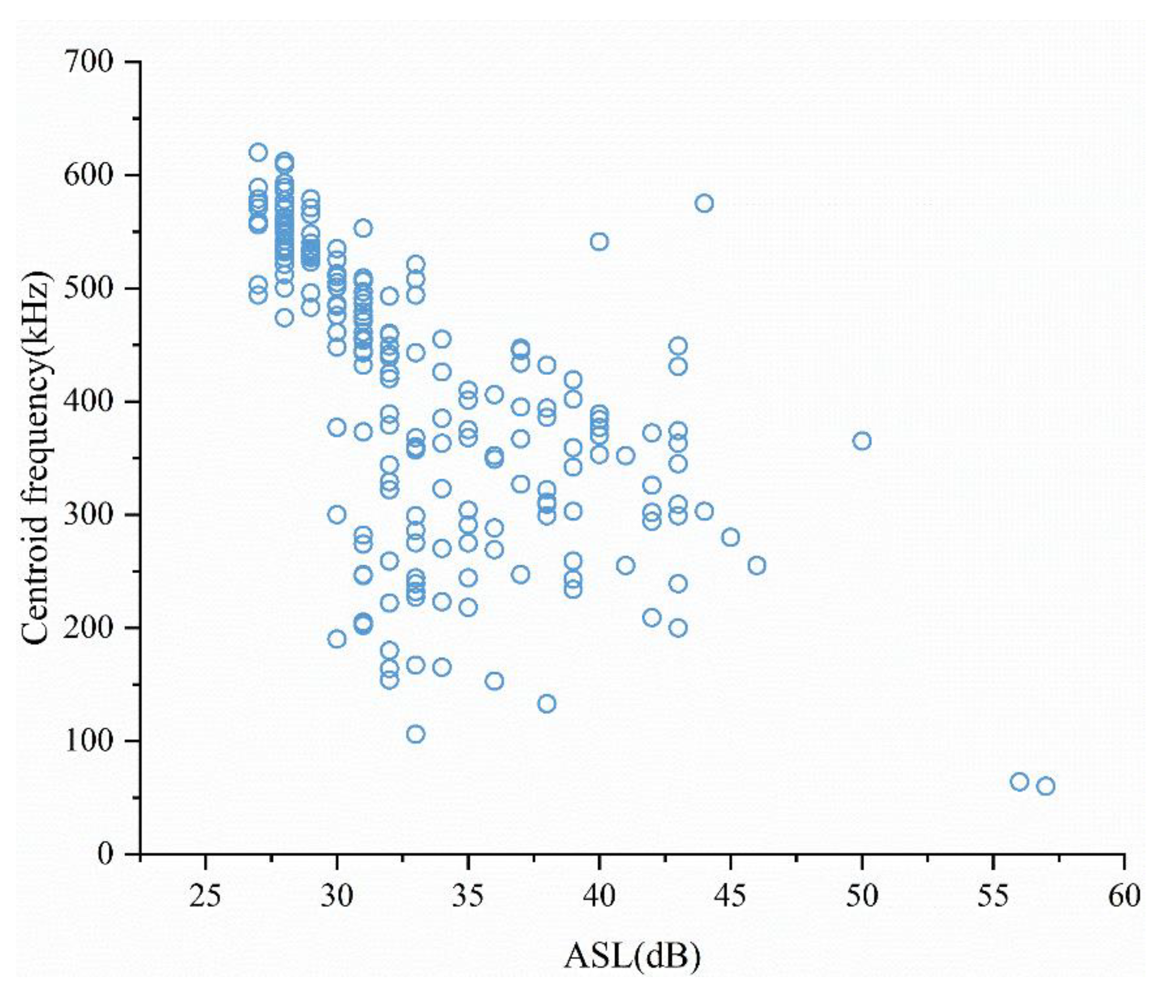
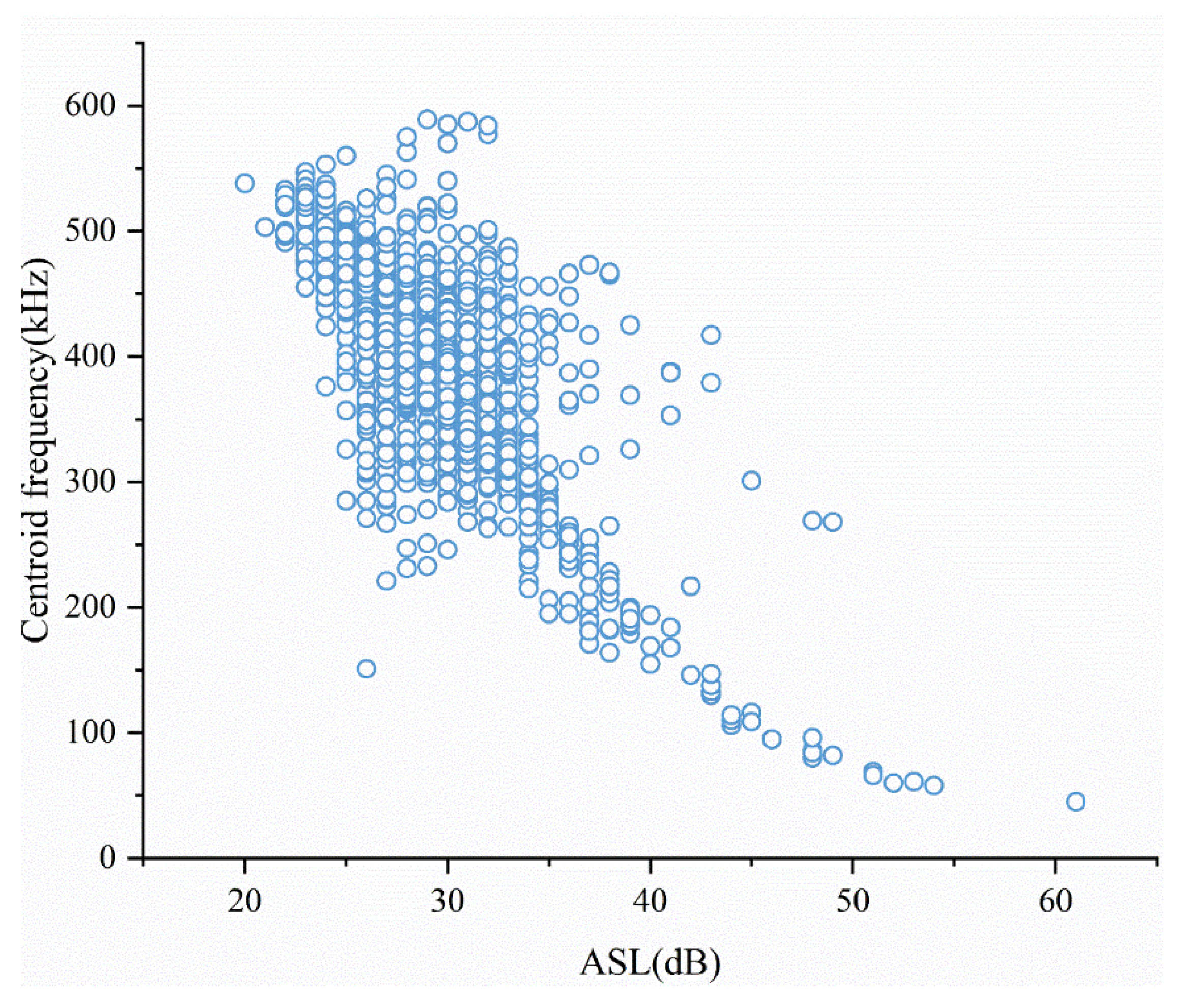
ASL-centroid frequency correlation analysis

The ASL of the signal represents the average signal amplitude in the time domain. The centroid frequency of the signal represents the location of the center of gravity of the signal frequency. The calculation is shown in Equation (4), where $f_x$ is the centroid frequency and $m_i$ is the amplitude at frequency $f_i$.

$$f_x=\frac{{\displaystyle \sum m_i{f}_i}}{{\displaystyle \sum m_i}}$$

(4)

ASL is the characteristic parameter in the time domain and the centroid frequency is the characteristic parameter in the frequency domain, respectively. Figure 25, Figure 26 and Figure 27 show their correlation analysis.

From the above figures, we find that the ASL of each bridge noise signal has a negative linear relationship with its centroid frequency. The larger the ASL, the smaller the centroid frequency. This indicates that the higher the amplitude level of the noise signal, the smaller the spectral distribution in the region. Moreover, the signal with a low signal amplitude level has wider spectral distribution.

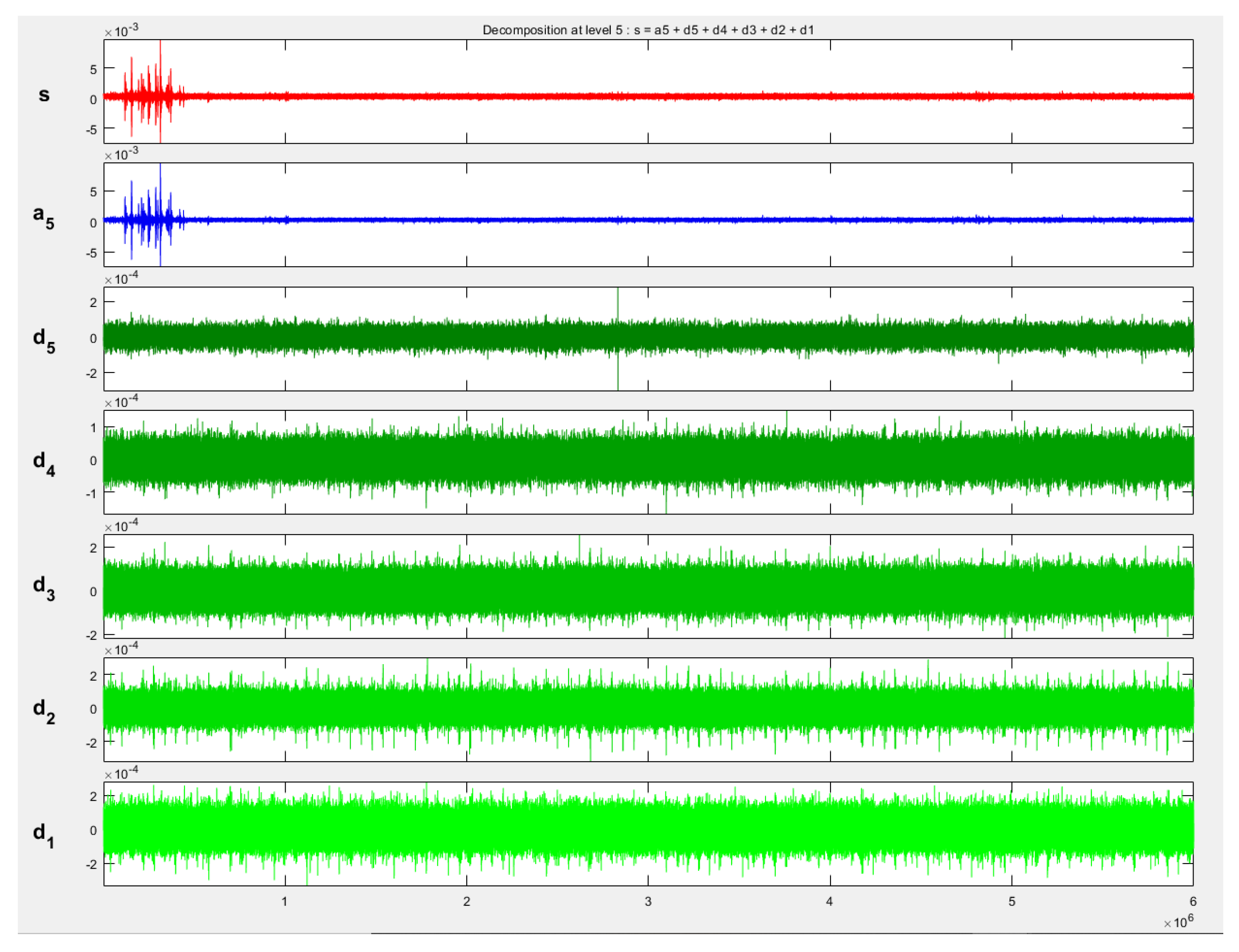
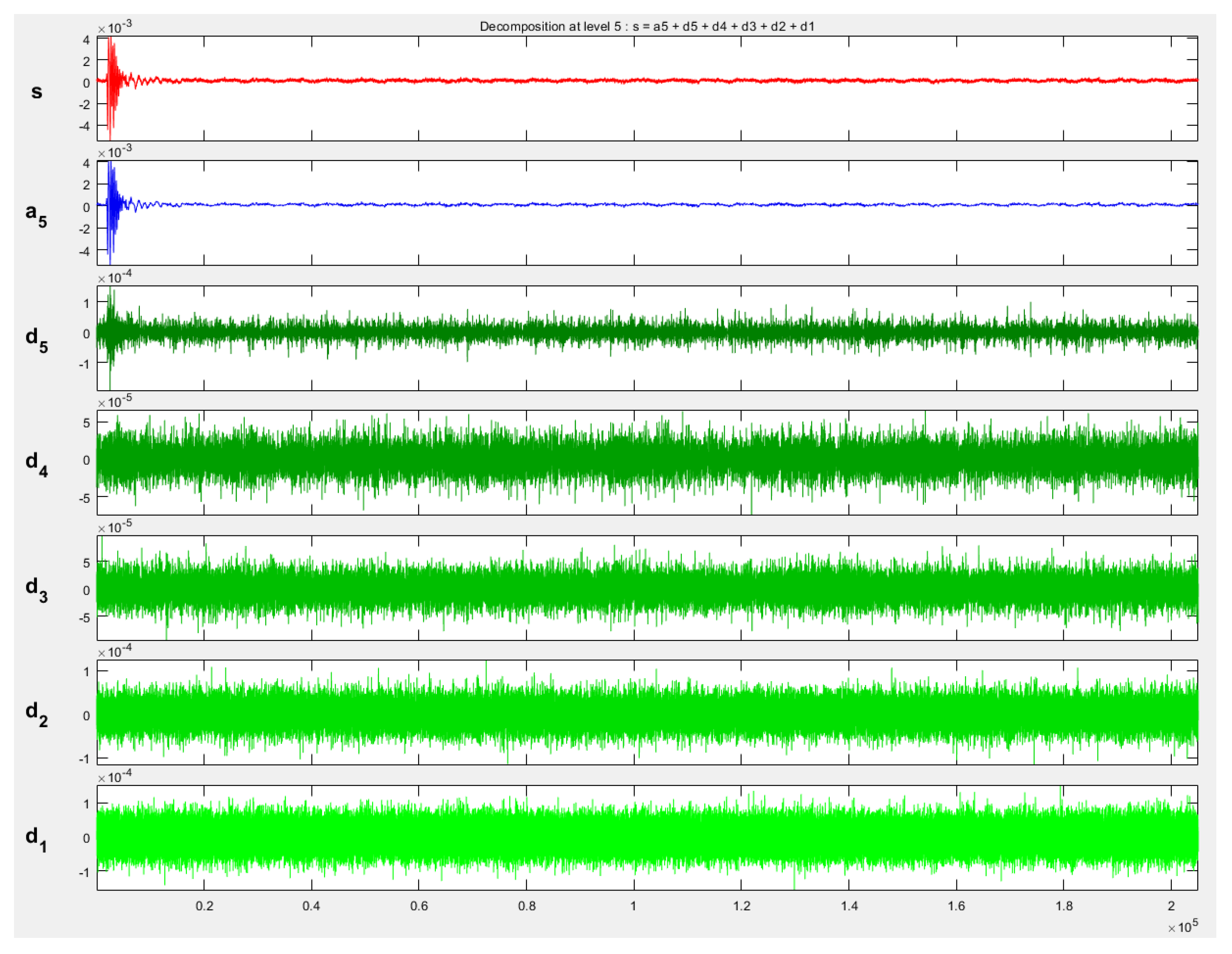
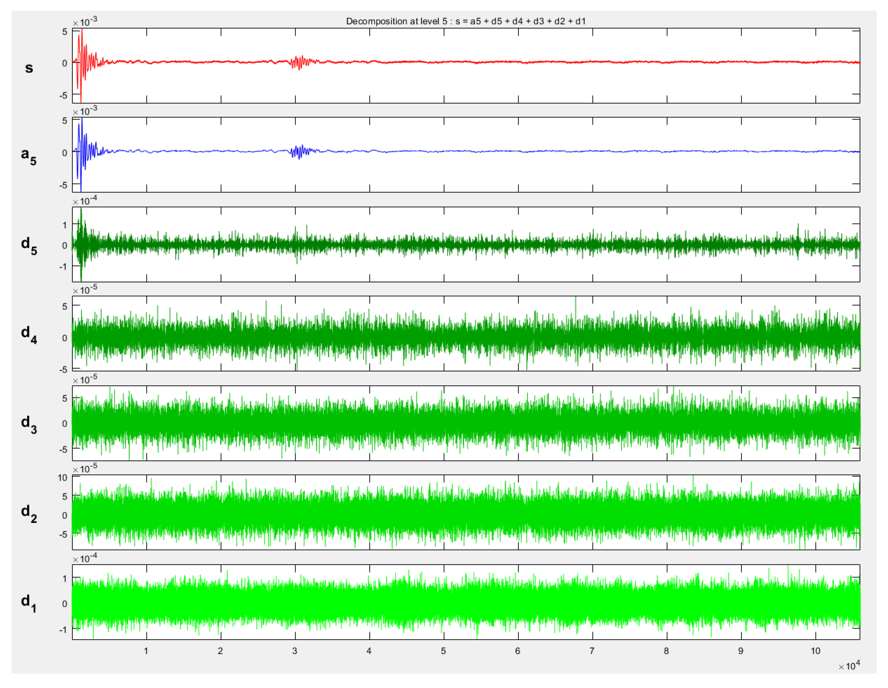
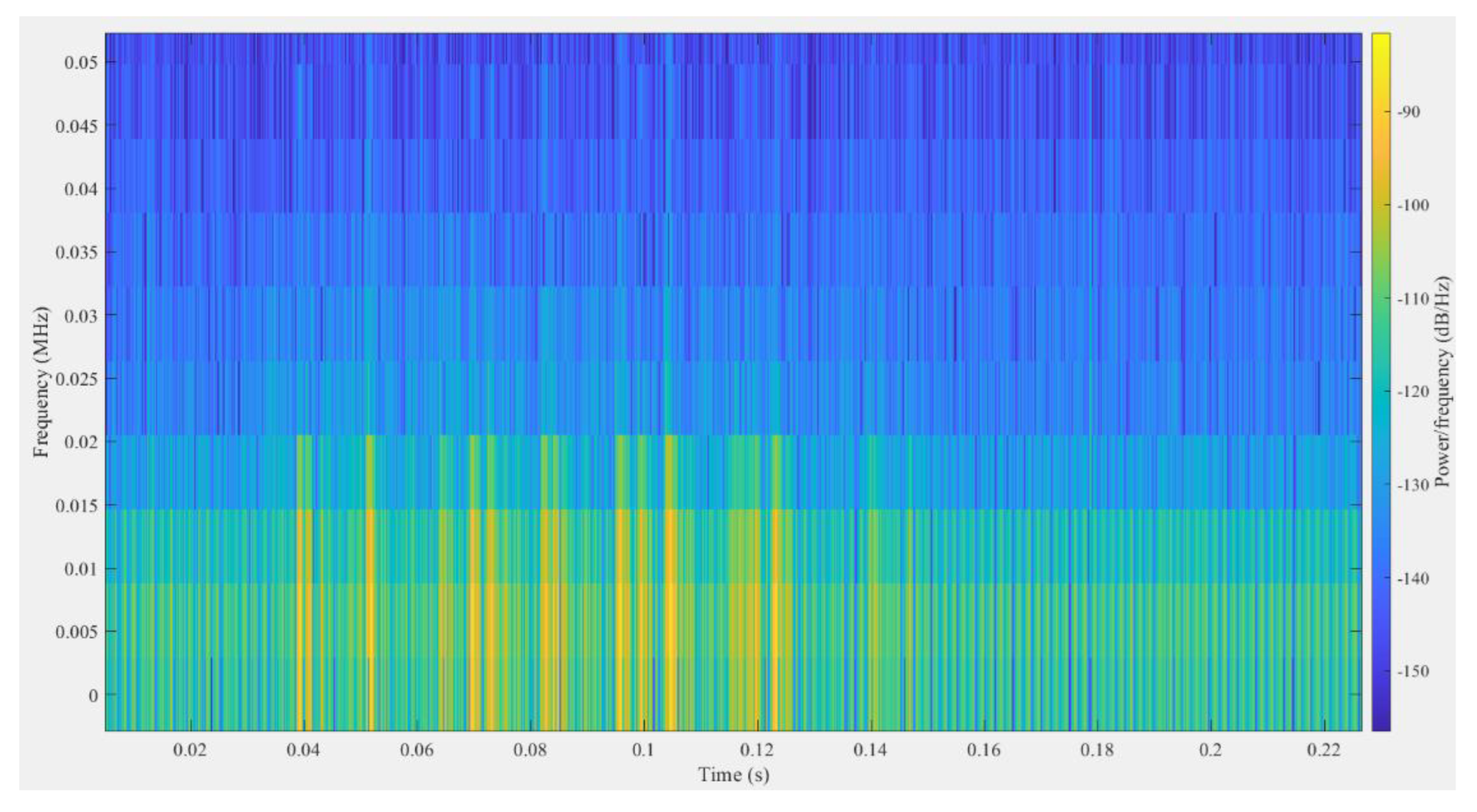
3.3.3. Wavelet Time-Frequency Analysis

The wavelet decomposition of the signals collected from the three bridges was performed using the wavelet basis functions and the number of decomposition layers determined above. Figure 28, Figure 29 and Figure 30 illustrate the signal wavelet transform decomposition.

The energy ratio of the decomposed layers is shown in

Table 2. Energy spectrum coefficient table of noise signal S1 of Yangma Island Bridge.

Wavelet Decomposition Parameters	a5	d5	d4	d3	d2	d1
Energy Spectrum Coefficient	98.17	0.20	0.19	0.48	0.38	0.59

,

Table 3. Energy spectrum coefficient table of noise signal S2 of Yellow River Bridge.

Wavelet Decomposition Parameters	a5	d5	d4	d3	d2	d1
Energy Spectrum Coefficient	98.72	0.18	0.01	0.12	0.23	0.68

and

Table 4. Energy spectrum coefficient table of noise signal S3 of Caihong Bridge.

Wavelet Decomposition Parameters	a5	d5	d4	d3	d2	d1
Energy Spectrum Coefficient	97.89	0.28	0.15	0.22	0.41	1.05

.

From the above waveform decomposition diagram, it can be observed that the amplitude of the signal is larger at low frequencies and smaller at high frequencies. Through the tables of energy spectrum coefficients of the decomposed signals of each layer, it can be observed that more than 97% of the energy of the noise signals of the three bridges are concentrated in the a5 layer, the low frequency part of the noise signals. The time-frequency analysis of the a5 part of each signal is conducted by short time Fourier transform (STFT), as shown in Figure 31, Figure 32 and Figure 33.

The above figures indicate that the signal energy of the noise signal with low frequency has a portion of more than 97%. The signal energy is concentrated in the frequency range up to 20 kHz by STFT. This frequency is also consistent with the signal frequency range analyzed above for the average frequency of the signal and the FFT transformations. The above rules and conclusions indicate that the frequency discrimination threshold for the noise signal in the health monitoring of bridge cables under real working conditions should be set to 20 kHz. The filter frequency is selected to be greater than 20 kHz, and the corresponding interference signal can be filtered out.

4. Conclusions

As a non-destructive testing method, AE technology has been widely used in many engineering fields. In this paper, an AE signal segmentation algorithm is proposed. The algorithm sets segmentation parameters to successfully segment a single AE signal in a continuous stream of acquired signals. The parameters include threshold, impact definition time, and impact blocking time. The proposed segmentation algorithm can not only facilitate the extraction of AE signal characteristics, but can also save 97.5% of storage space. This may greatly improve the application of AE technology in the health monitoring of bridge cables.

To solve the problem of the lack of study of the noise properties under real environments, experiments have been conducted in three different bridges. The experimentally acquired 5611 noise signals have been synthesized and analyzed in the time domain, frequency domain and wavelet time-frequency domain. The analysis reveals that the main characteristic parameter ranges of the noise signals of the three bridges are relatively consistent. The main cause of noise generation is vehicles passing by. The amplitude threshold of the experimentally obtained noise signal is 80 dB, the duration threshold is 0.15 s, the energy threshold is 1000 ms*mV, and the ringing count threshold is 1000 times, respectively. The average frequency of the noise signal is within 20 kHz, as determined by frequency domain analysis. In addition, 97% of the signal energy is mainly concentrated in 20 kHz, as determined by wavelet analysis and STFT analysis. According to the noise signal characteristic parameter derived from the above three real working condition experiments, the noise can be efficiently filtered and identified during or after the signal acquisition. Future studies will be conducted to investigate the probabilistic distribution of AE energies based on the collected data. Some previous work has provided effective approaches to this aspect, such as [28,29]. The additional data analysis will allow for a deeper analysis of the mechanisms in the metals.

References

1. Deng, B. Application of bridge health monitoring system in a bridge. China Sci. Technol. Inf. 2021, 18, 71–74. [Google Scholar]
2. Yuan, G.; Zhang, C.X.; Hu, S.L. Big Data Based Bridge Anomaly Detection and Situational Awareness. In Proceedings of the 2019 Chinese Automation Congress (CAC), Hangzhou, China, 22–24 November 2019; pp. 3864–3868. [Google Scholar]
3. Wang, D.L.; Zhang, Y.Q.; Pan, Y. An Automated Inspection Method for the Steel Box Girder Bottom of Long-Span Bridges Based on Deep Learning. IEEE Access 2020, 8, 4010–4023. [Google Scholar] [CrossRef]
4. Zeng, Z.W. Study on the application of nondestructive testing technology in bridge road engineering. Transp. Manag. World 2020, 9, 61–62. [Google Scholar]
5. Sherine, M.E.; Kumari, S.L. Study of acoustic emission signals in continuous monitoring: A review. In Proceedings of the International Conference on Circuit Power and Computing Technologies, Kollam, India, 20–21 April 2017; pp. 1–8. [Google Scholar]
6. Li, D.S.; Hu, Q. Wavelet analysis of fatigue damage acoustic emission signal of carbon fiber bridge cables. Disaster Prev. Mitig. Eng. J. 2010, 30, 318–322. [Google Scholar]
7. Hu, Q. Fatigue Acoustic Emission Signal Processing and Damage Analysis of Bridge Cables; Dalian University of Technology: Dalian, China, 2011. [Google Scholar]
8. Yapar, O.; Basu, P.K.; Volgyesi, P. Structural health monitoring of bridges with piezoelectric AE sensors. Eng. Fail. Anal. 2015, 56, 150–169. [Google Scholar] [CrossRef] [Green Version]
9. Xin, G.L. Research on the Identification Method of Bridge Cable Breakage Signal Based on Acoustic Emission Technology; Shandong University: Jinan, China, 2020. [Google Scholar]
10. Ren, B.; Chen, J. Fracture acoustic emission signals identification of broken wire using deep transfer learning and wavelet analysis. In Proceedings of the International Conference on Artificial Intelligence and Information Systems, Tangerang Selatan, Indonesia, 29–30 June 2021; Volume 30. [Google Scholar]
11. Carrion-Viramontes, F.J.; Hernandez-Figueroa, J.A.; Machorro-Lopez, J.M. Weld acoustic emission inspection of structural elements embedded in concrete. Sci. Prog. 2022, 105, 368504221075482. [Google Scholar] [PubMed]
12. Sarfarazi, V.; Fattahi, S.; Asgari, K.; Bahrmi, R.; Wang, X. Failure Behavior of Room and Pillar with Different Room Configuration Under Uniaxial Loading Using Experimental Test and Numerical Simulation. Geotech. Geol. Eng. 2014, 40, 2881–2896. [Google Scholar] [CrossRef]
13. Sarfarazi, V.; Tabaroei, A.; Asgari, K. Discrete element modeling of strip footing on geogrid-reinforced soil. Geomech. Eng. 2022, 29, 435–449. [Google Scholar]
14. Sarfarazi, V.; Haeri, H.; Asgari, K. Three-dimensional Discrete Element Simulation of Interaction between Aqueduct and Tunnel. Period. Polytech. Civ. Eng. 2022, 66, 30–39. [Google Scholar]
15. Li, D.S.; Ou, J.P.; Lan, C.M.; Li, H. Monitoring and failure analysis of corroded bridge cables under fatigue loading using acoustic emission sensors. Sensors 2012, 12, 3901–3915. [Google Scholar] [CrossRef] [PubMed]
16. Gaillet, L.; Zejli, H.; Laksimi, A.; Tessier, C.; Drissi-Habti, M.; Benmedakhene, S. Detection by acoustic emission of damage in cable anchorage. In Proceedings of the Non-Destructive Testing in Civil Engineering, Nantes, France, 30 June–3 July 2009. [Google Scholar]
17. Papacharalampopoulos, A.; Stavropoulos, P.; Doukas, C.; Foteinopoulos, P.; Chryssolouris, G. Acoustic emission signal through turning tools: A computational study. Procedia CIRP 2013, 8, 426–431. [Google Scholar] [CrossRef] [Green Version]
18. Stavropoulos, P.; Papacharalampopoulos, A.; Vasiliadis, E.; Chryssolouris, G. Tool wear predictability estimation in milling based on multi-sensorial data. Int. J. Adv. Manuf. Technol. 2016, 82, 509–521. [Google Scholar] [CrossRef] [Green Version]
19. Zhou, Z.L.; Zhou, J.; Cai, X. Acoustic emission source location considering refraction in layered media with cylindrical surface. Trans. Nonferrous Met. Soc. China 2020, 30, 789–799. [Google Scholar] [CrossRef]
20. Jennings, S.J.; Wu, T.; Regez, B. A Review on Effective Acoustic Emission. In Proceedings of the International Conference on Micro/Nano Sensors for Artificial Intelligence, Healthcare, and Robotics (NSENS), Shenzhen, China, 31 October–2 November 2019; pp. 113–118. [Google Scholar]
21. Rastegaev, I.A.; Danyuk, A.V.; Merson, D.L. Universal Educational and Research Facility for the Study of the Processes of Generation and Propagation of Acoustic Emission Waves. Inorg. Mater. 2017, 15, 1548–1554. [Google Scholar] [CrossRef]
22. Meng, X.; Liu, W.; Ding, E. The Research of Acoustic Emission Signal Classification. In Proceedings of the International Conference on Intelligent Information Hiding and Multimedia Signal Processing, Dalian, China, 14–16 October 2011; pp. 41–44. [Google Scholar]
23. Xu, C.L.; Li, G.L.; Dong, T.S. Research progress of acoustic emission signal analysis and processing methods. Mater. Guide 2014, 28, 56–60. [Google Scholar]
24. Liu, K.L. Acoustic Emission Feature Extraction of Axle Cracks Based on Parametric Analysis; Dalian Jiaotong University: Dalian, China, 2017. [Google Scholar]
25. Zhang, Y.B.; Wu, W.R.; Yao, X.L. Study on Spectrum Characteristics and Clustering of Acoustic Emission Signals from Rock Fracture. Circuits Syst. Signal Process. 2020, 39, 1133–1145. [Google Scholar] [CrossRef]
26. Nikkhah, M.; Goshatasbi, K.; Ahangari, K. Application of wavelet transform in evaluating the Kaiser effect of rocks in acoustic emission test. Measurement 2022, 192, 110887. [Google Scholar]
27. Yao, J. Research on the Detection of Broken Gear Teeth Based on Acoustic Emission Technology; Southwest University of Science and Technology: Mianyang, China, 2020. [Google Scholar]
28. Salje, E.K.; Dahmen, K.A. Crackling noise in disordered materials. Annu. Rev. Condens. Matter Phys. 2014, 5, 233–254. [Google Scholar] [CrossRef]
29. Chen, Y.; Gou, B.; Yuan, B.; Ding, X.; Sun, J.; Salje, E.K. Multiple Avalanche Processes in Acoustic Emission Spectroscopy: Multibranching of the Energy—Amplitude Scaling. Phys. Status Solidi B 2022, 259, 2100465. [Google Scholar] [CrossRef]
Figure 1. Acoustic emission simplified waveform characteristic parameter model.
Applsci 12 06727 g001
Figure 2. Flow chart of acoustic emission signal segmentation algorithm.
Applsci 12 06727 g002
Figure 3. Experiment site: (a) panoramic view of Yangma Island Bridge; (b) device connection.
Applsci 12 06727 g003
Figure 4. Experiment site: (a) panoramic view of Jinan Yellow River Bridge; (b) device connection.
Applsci 12 06727 g004
Figure 5. Experiment site: (a) panoramic view of Shen Zhen Caihong Bridge; (b) device connection.
Applsci 12 06727 g005
Figure 6. Acquired continuous signal waveform.
Applsci 12 06727 g006
Figure 7. Segmented acoustic emission signal. (a) Signal 1; (b) Signal 2; (c) Signal 3; (d) Signal 4; (e) Signal 5.
Applsci 12 06727 g007
Figure 8. Impact-amplitude correlation diagram of cable noise signal of Yangma Island Bridge.
Applsci 12 06727 g008
Figure 9. Impact-amplitude correlation diagram of cable noise signal of Yellow River Bridge.
Applsci 12 06727 g009
Figure 10. Impact-amplitude correlation diagram of cable noise signal of Caihong Bridge.
Applsci 12 06727 g010
Figure 11. Ring count-duration correlation diagram of cable noise signal of Yangma Island Bridge.
Applsci 12 06727 g011
Figure 12. Ring count-duration correlation diagram of cable noise signal of Yellow River Bridge.
Applsci 12 06727 g012
Figure 13. Ring count-duration correlation diagram of cable noise signal of Caihong Bridge.
Applsci 12 06727 g013
Figure 14. Amplitude-energy correlation diagram of cable noise signal of Yangmadao Bridge.
Applsci 12 06727 g014
Figure 15. Amplitude-energy correlation diagram of cable noise signal of Yellow River Bridge.
Applsci 12 06727 g015
Figure 16. Amplitude-energy correlation diagram of cable noise signal of Caihong Bridge.
Applsci 12 06727 g016
Figure 17. Noise signal impact-vehicle counting correlation diagram at position 1 of Yellow River Bridge.
Applsci 12 06727 g017
Figure 18. Noise signal impact-vehicle counting correlation diagram at position 2 of Yellow River Bridge.
Applsci 12 06727 g018
Figure 19. Time domain and frequency domain waveform diagram of noise signal of Yangma Island Bridge. (a) Signal time domain diagram; (b) signal frequency domain diagram.
Applsci 12 06727 g019
Figure 20. Time domain and frequency domain waveform diagram of noise signal of Yellow River Bridge. (a) Signal time domain diagram; (b) signal frequency domain diagram.
Applsci 12 06727 g020
Figure 21. Time domain and frequency domain waveform diagram of noise signal of Caihong Bridge. (a) Signal time domain diagram; (b) signal frequency domain diagram.
Applsci 12 06727 g021
Figure 22. Average frequency-energy correlation diagram of noise signal of Yangma Island Bridge.
Applsci 12 06727 g022
Figure 23. Average frequency-energy correlation diagram of noise signal of Yellow River Bridge.
Applsci 12 06727 g023
Figure 24. Average frequency-energy correlation diagram of noise signal of Caihong Bridge.
Applsci 12 06727 g024
Figure 25. ASL-centroid frequency correlation diagram of Yangma Island Bridge.
Applsci 12 06727 g025
Figure 26. ASL-centroid frequency correlation diagram of Yellow River Bridge.
Applsci 12 06727 g026
Figure 27. ASL-centroid frequency correlation diagram of Caihong Bridge.
Applsci 12 06727 g027
Figure 28. Waveform decomposition diagram of noise S1.
Applsci 12 06727 g028
Figure 29. Waveform decomposition diagram of noise S2.
Applsci 12 06727 g029
Figure 30. Waveform decomposition diagram of noise S3.
Applsci 12 06727 g030
Figure 31. Time-frequency diagram of low frequency signal in S1 noise signal.
Applsci 12 06727 g031
Figure 32. Time-frequency diagram of low frequency signal in S2 noise signal.
Applsci 12 06727 g032
Figure 33. Time-frequency diagram of low frequency signal in S3 noise signal.
Applsci 12 06727 g033