Abstract
To prevent lifetime shortening and premature failure in turbine runners, it is of paramount importance to analyse and understand its dynamic response and determine the factors that affect it. In this paper, the dynamic response of a Kaplan runner is analysed in air by numerical and experimental methods. First, to start the analysis of Kaplan runner mode shapes, its geometry is simplified and modelled as a bladed disk. Bladed disks with different blade numbers are investigated, by numerical simulation, in order to understand the influence of this parameter on its modal characteristics. Then, mode shapes extracted are characterized and a classification is proposed. Second, an existing Kaplan runner is simulated by Finite Elements Method (FEM) and its mode shapes are extracted. The obtained results are contrasted with the bladed disks mode shapes, in order to validate the classification proposed. The simulated Kaplan runner is also experimentally studied. A numerical modal analysis is carried out in the real runner. Different, global and local, mode shapes are identified. The global mode shapes extracted by numerical and experimental modal analysis are compared and discussed. Finally, the local mode shapes identified are commented and explained by means of numerical simulation.
1. Introduction
In recent years, new renewable energies (NRE), such as wind and solar, have experienced a strong entry into power generation [1,2]. Because the energy generated is random in nature, NRE can produce grid instabilities. Hydropower plants are the only ones that generate different levels of power depending on the demand for electricity (the generation has to match the demand for the stability of the electricity grid). As a result of this flexibility, hydroelectric power is an ideal complement to NREs. Because of this, hydraulic turbine units often undergo frequent start and stop cycles [3] and operate under out-of-design operating conditions. When the machine works in these operating conditions, fluid instabilities are induced. Due to this, turbulence and high-level pressure pulsations due cavitation, load variation and rotor-stator interaction can lead to undesirable excitations in the runner. These excitations can generate high vibration amplitudes in the runner, which can induce a useful life shortening or a premature failure in the worst cases [4,5,6,7,8,9,10]. In order to avoid the critical operating conditions, it is of paramount importance to analyze the dynamic response of the runners.
Many investigations were carried out to understand the dynamic response of the turbine runners and the parameters that affect it. For instance, Liang et al. [11] made a numerical modal analysis of a Francis runner considering the added mass effect. The mode shapes and natural frequencies were extracted in this study. Even though the natural frequencies calculated decrease significantly when the runner is submerged in water, the mode shapes undergo only small changes. Rodriguez et al. [12] made an experimental study about the added mass effect on a Francis runner in still water. It was found that the frequency decrease of a submerged Francis runner is caused by the added mass. In these works, it can be noticed that the mode shapes of the runner, extracted by numerical methods and experimentally, are mainly dominated by the deformation of the band and the blades. The global shape of these vibration modes can be found in simpler geometries, such as a thick-walled circular cylinder, like the one studied by Singhal et al. [13].
Similarly, for experimental procedures and analytical studies, it can be convenient to analyze simplified models of complex structures with similar dynamic response. Huang et al. [14] studied the dynamic behaviour of a pump-turbine runner by numerical simulation. The runner was modeled as a disk-blade-disk structure that had the same mode shapes. It was concluded that the blade number and the shape of the blades can modify the natural frequencies depending on the mode shape. Even simpler geometries were used to model these kinds of runners. For instance, Presas et al. [15] studied experimentally and analytically a rotating and submerged disk. In that study the rotation effects on the submerged disk and the transmission of the vibration to the casing were studied. The natural frequencies and mode shapes were measured from the casing. Valentín et al. [16] made an experimental study about the effect of the casing in a submerged disk, in order to understand the effect of a rigid and a flexible enclosure. It was found that while frequencies of the disk decrease when the disk gets close to the rigid wall, the opposite occurs when the disk gets close to the non-rigid wall. Louyot et al. [17] made a modal analysis of a spinning disk in a dense fluid as a model for a high-head hydraulic runner. The mode shapes were extracted and, an expression for co- and counter-rotating wave angular frequency was analytically determined.
For the study of the dynamic response of Kaplan runners, the numerical simulation of the Kaplan turbine is often built and just a few mode global mode shapes are described [18,19,20,21,22]. According to the author’s knowledge, no general description of the mode shapes of a Kaplan runner exist.
In this paper the global mode shapes of Kaplan runners are investigated. To explore the runner mode shapes, a simple model of the runner is considered (bladed disk). Bladed disks with different blade number are studied by numerical simulation. The mode shapes are characterized and a classification is carried out. These results are compared with the mode shapes obtained by the numerical simulation of a real Kaplan and are contrasted with the mode shapes extracted from the experimental data. It is important to remark that this study considers the mode shapes of the runner without the effects of rotation or water added mass. Nevertheless, as pointed out by some researchers, these effects do not substantially modify the mode shapes and therefore the conclusions obtained here can be applied to describe the dynamic response of Kaplan runners.
2. Numerical and Experimental Modal Analysis
The relation between the excitation and the response of the structure is called Frequency Response Function (FRF).
According to the modal analysis theory, every structure can be modelled as a combination of masses, dampers and springs, which are interconnected with each other. The equation of motion of a system with n degrees of freedom, which is excited with a time-dependent force, is given by:
where x, and are displacement, velocity and acceleration vectors, respectively, in the time domain. [M], [C] and [K] are the mass, damping and stiffness matrix of the system. F is the excitation force applied to each degree of freedom.
To obtain the FRF, Equation (1) has to be transformed from the time domain to the frequency domain. Thus, the Fourier transform is applied to this equation as follows:
where {X(jω)} and {F(jω)} are the above time-dependent displacement and force vectors, respectively, in the frequency domain. [H(jω)] is the frequency response function, which relates each element of the excitation vector to each element of the displacement vector.
When a FEM modal analysis is carried out, Equation (1) is often solved as an undamped system, which means [C] = 0. Natural frequencies and mode shapes are calculated from this model. Then, an individual modal damping factor ξ may be added to each vibration mode to later calculate the damped natural frequencies. The mode shapes do not change by adding this damping factor. Then, the mode shapes of the undamped system are used in this damped system model [23].
Many real structures are considered proportionally damped structures. The proportional damping model defines the damping coefficient matrix as a linear combination of the mass and the stiffness matrixes. The FRF for this kind of damped structures is given by [24]:
In Equation (3), N is the number of vibration modes of the system. Then, this equation shows a superposition of all vibration mode shapes excited by an external force. Then, for each mode r:
- ωr is the natural frequency of the corresponding vibration mode.
- θr is the damping factor of the structure.
- {θ}r is the vibration mode shape that dominates the structure near a resonance condition (ωexcitation = ωr).
- Qr is the scaling factor, which is a constant value for each mode shape.
Even though in Equation (2) the excitation force is related to the displacement, the FRF can be represented as:
- Receptance function: relation between the displacement and the excitation force.
- Mobility function: relation between the velocity and the excitation force.
- Inertance function: relation between the acceleration and the excitation force.
These three transfer functions are related to each other, as is shown in Equation (4). These transfer functions are equally valid forms of the frequency response function.
3. Natural Frequencies and Mode Shapes of Simplified Structures
As mentioned before, to understand the modal characteristics of complex geometry structures it is often convenient to model these structures as simplified geometries with similar mode shapes. In this section, some simple geometries are analyzed and discussed in order to have a better comprehension of the mode shapes of a Kaplan runner.
3.1. Modal Characteristics of a Disk-like Structure
A basic disk, defined by a radius r and a thickness h, is often used as a simplified model of some types of runners. In free vibration condition, its motion is governed by the following differential equation (in polar coordinates) [25]:
where: ρ is the density, w is the transverse displacement, t is the time, E is the Young modulus and ν is the Poisson coefficient. On one hand, by solving equation (5), the transverse displacement w can be analytically determined [25,26,27].
On the other hand, natural frequencies and mode shapes can also be obtained by performing a numerical modal analysis.
As a starting point of this study, a basic disk model, clamped at its center, is analyzed. This disk has an outer diameter D = 400 mm, an inner diameter d = 40 mm and a thickness h = 8 mm (See Figure 1a). To perform a numerical modal analysis a mesh with 41850 hexahedral elements (with a size of 3 mm) is used (see Figure 1b). Moreover, a Fixed Support condition is used and placed in the center of the disk.
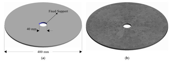
Figure 1.
Disk: (a) Geometry and fixed support location, (b) Mesh.
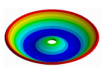
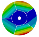
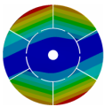
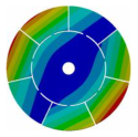
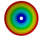
From here, mode shapes and natural frequencies of the disk are obtained. In Table 1 some mode shapes of a disk clamped at its center are shown and sorted by the number of nodal diameters (D) and nodal circles (C). As it was studied by many authors [17,26,28,29,30,31], the vibration mode shapes of a disk have combinations of nodal diameters and nodal circles, which increase their number with the mode order. For convenience, in this work, the mode shapes related to the disk will be called modes “(m, n)” for modes shapes with m nodal diameter and n nodal circles.

Table 1.
Vibration mode shapes of a disk clamped at its center.
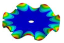
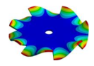
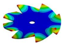
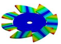
3.2. Transition from a Disk to a Bladed Structure
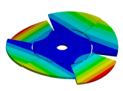
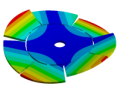
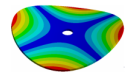
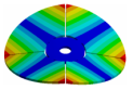
To understand the global mode shapes of a bladed structure, it is proposed to study different transition geometries starting from a basic disk. In order to get the shape of a bladed structure with mode shapes similar to a Kaplan runner, the basic disk of Figure 1 is progressively modified. Figure 2a–e shows the steps used to create a blade from a disk section. The three lengths (L1, L2 and L3), indicated in Figure 2f, are the main dimensions of the blade and are defined by:
where Z is the number of blades, δ is the cut width (1% of D), b is the blade root width (5% of D) and λ is the aspect ratio of the blade. For the following models, an aspect ratio λ = 2.3 is used. This value is obtained from a real Kaplan blade, which is used as reference geometry.
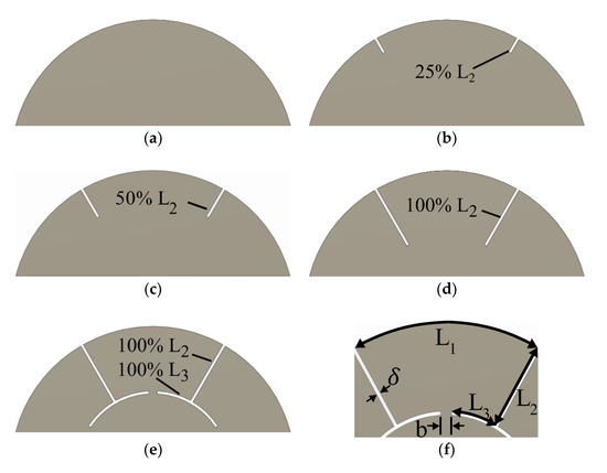
Figure 2.
Stages from the basic disk section to the blade shape: (a) Basic disk section, (b) Transition 1, (c) Transition 2, (d) Transition 3, (e) Final blade model, (f) Blade main dimensions.
Once the lengths of the cuts and the blade number are defined, the final geometries of the models to study are obtained. Table 2 shows the disk, the transition structures and the final model for a bladed structure with 4 blades, as an example of the explained procedure.
Table 2.
Progressive modification from the disk to a bladed structure (Z = 4).
3.3. Influence of the Blade Number on the Mode Shapes
This section aims to investigate the influence of the blade number on the Kaplan runner mode shapes. Bladed disks with 4 to 7 blades are studied. Each bladed disk is analyzed from the basic disk geometry, as it was explained in the above section. The detail of the geometry of the models can be seen in Appendix A, in Table A1. Using the same boundary conditions and mesh characteristics used for the disk simulation, a numerical modal analysis is carried out for each model. Then, the mode shapes and natural frequencies are extracted.
3.3.1. Mode Shapes Due to the Clamping
The first modes to analyze are mode (1,0) and (0,0), which are the modes related to the clamping condition at the center of each model [32].
In Table 3, the basic disk and the bladed disk models are shown, at the vibration mode (1,0). It is possible to see that the bladed disk becomes more similar to the disk, in this vibration mode, at a higher blade number. When the blade number is even, a blade and the blade at its counter side vibrate at the same amplitude (see Z = 4 in Table 3). But the next blade and the blade at its counter side vibrate at a different amplitude, in order to match the mode shape with the geometry of the model (see Z = 6 in Table 3). In contrast, if the blade number is odd, to match the structure geometry with the vibration mode shape, each blade may have a different vibration amplitude and deformation distributions (see Z = 5 and Z = 7 in Table 3).
Table 3.
Mode (1,0) for bladed disk models.
The detail of the transition of the mode from the disk to the geometries shown in this table can be seen in Appendix B, in Table A2.
In Table 4 the basic disk and the bladed disk models are shown, at the mode (0,0). In this case, in contrast to the mode (1,0), it is clear that the geometry of the structure is compatible with the mode shape. The mode (0,0) is not affected by the blade number. All the blades, in every model, vibrate with the same amplitude and in-phase with respect to the other blades.
Table 4.
Mode (0,0) for every bladed disk model.
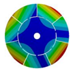
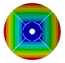
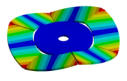
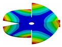
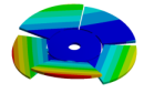
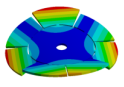
3.3.2. Diametrical Mode Shapes of Bladed Disks
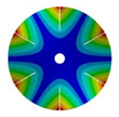
According to the literature [27], after a numerical modal analysis is performed, a pair of diametrical mode shapes is extracted at the same natural frequency. These modes have the same mode shape but different angular orientations, as shown in the “Disk” column in Table 5, Table 6, Table 7, Table 8, Table 9 and Table 10. But then, when the disk is progressively modified, the equal diametrical mode pair of the disk become two different global modes in the bladed disk (see the aforementioned tables).
Table 5.
Mode (2,0) for a bladed disk with Z = 4.
Table 6.
Mode (3,0) for a bladed disk with Z = 6.
Table 7.
Mode (4,0) for a bladed disk with Z = 4.
Table 8.
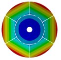
Mode (6,0) for a bladed disk with Z = 6.
Table 9.
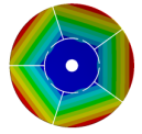
Mode (5,0) for a bladed disk with Z = 5.
Table 10.
Mode (7,0) for a bladed disk with Z = 7.
To understand the influence of the blade number on the global modes of the bladed disk, the diametrical modes of the disk are studied. For this, and in order to have a global view of this influence, the bladed disks are analysed as bladed disks with an even blade number (Z = 4 and Z = 6) or odd blade number (Z = 5 and Z = 7).
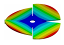
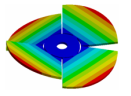
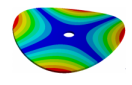
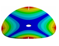
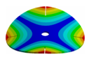
Global mode shapes of the bladed disk are generated when the “disk mode shapes” match the blade disk geometry. The first example is shown in Table 5. In this table, the transition from a disk to a bladed disk with Z = 4, at the mode (2,0), is shown. Here, it is possible to see that the nodal diameters are placed in two main directions: Between the blades (Table 5, row 1) and across the blades (Table 5, row 2). When the nodal diameter passes through the blade, the vibration of each blade is associated with a torsional movement. In contrast, when the nodal diameter is placed in between the blades, the vibration of each blade is associated with a bending movement.
The same effect occurs when a bladed disk with Z = 6 vibrates at the mode (3,0) (see Table 6). In here, the torsional and bending vibrations in the blades are also determined by the position of the nodal diameters with respect to them.
Then, when the number of nodal diameters is half the number of blades (), the global mode shapes are associated with a bending mode shape and a torsional mode shape of the blades. Furthermore, as it can be seen in the “Bladed Disk” column in Table 5 and Table 6, each blade moves in counter-phase with respect to the next blade.
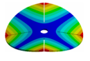
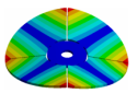
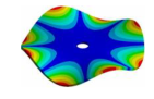
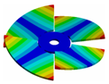
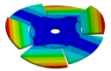
Now, when the bladed disk with Z = 4 vibrates in the mode (4,0), as shown in Table 7, the geometry of the structure and the number of nodal diameters distribution are also compatible. It can be seen that mode shapes of the bladed disk are also dependent on the orientation of the nodal diameters. In this case, also two orientations are possible. In the first one, the nodal diameters pass through the blades and in between them, which is related to a torsional vibration of each blade as a rigid body. In the second orientation, the nodal diameters pass only through the blades. A torsional vibration with two torsional axes on each blade is associated with this orientation (See Table 7, second row, “Bladed Disk” column).
As is shown in Table 8, for a bladed disk, with Z = 6, vibrating at the mode (6,0), the global mode shapes are similar to the previous case. In general, when the number of nodal diameters is equal to the number of blades (m = Z) torsional global mode shapes of the bladed disk are generated. In contrast to the case of the modes (m = Z/2, 0), in this case, every blade vibrates in-phase with respect to the next blade.
It is important to remark that in a bladed disk with an even blade number, global mode shapes that show a uniform deformation distribution of the blades are generated for every m = (k*Z)/2 nodal diameters, with k = 1,2,3…
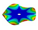
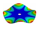
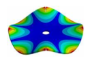
In Table 9 and Table 10, bladed disks with an odd number of blades are shown (Z = 5 and Z = 7). In both cases, the number of nodal diameters is equal to the number of blades (m = Z). Then, the same torsional global modes described before are present in these cases.
Hence, for a bladed disk with an odd blade number, the diametrical global mode shapes that show a uniform deformation distribution of the blades is generated for m = k*Z nodal diameters, with k = 1, 2, 3…
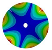
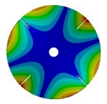
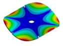
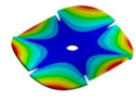
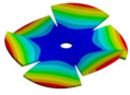
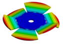
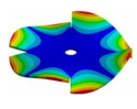
Finally, since the non-uniform deformation distribution mode shapes are also present in Kaplan runners, the cases when the nodal diameter distribution is not compatible with the bladed disks geometry are also studied. In Table 11 and Table 12, the modes (2,0) and (3,0), are shown for every bladed disk, respectively. It is possible to see that the nodal diameters of the modes are redistributed, in order to match the structure geometry with the mode shape. In this kind of mode shapes, not only different amplitude of the blades with respect to the others exists, but also different mode shapes of the blade can be seen in the bladed disk. For instance, in Table 11 columns Z = 6 and Z = 7, bending and torsion mode shapes of the blade coexist in the mode (2,0) of the bladed disk. Due to the blade number influence, the modes (2,0) and (3,0) are present in every bladed disk as a global mode shape but with a non-uniform behaviour of the blades, with the exception of the bladed disk with Z = 4 and Z = 6, respectively. The detail of the transition of the mode shapes from the disk to the different bladed disks, can be seen in Appendix B, in Table A3 and Table A4. It may be useful to the reader to have a better comprehension of the nodal diameters distribution in Table 11 and Table 12.
Table 11.
Mode (2,0) for every bladed disk.
Table 12.
Mode (3,0) for every bladed disk.
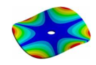
3.3.3. Circular Mode Shapes of Bladed Disks
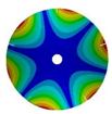
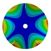
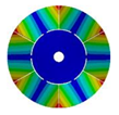
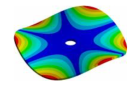
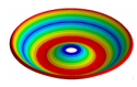
Besides the diametrical mode shapes, the first circular mode shape is studied. The mode (0,1) is shown in Table 13 for all the bladed disk models. As the mode (0,0), the geometry of the mode shape is compatible with any circular structure. This mode shape is not affected by the blade number, so, circular global mode shapes exist for any n number of nodal circles.
Table 13.
Mode (0,1) for every bladed disk model.
It is worth noting that all of the higher-order global modes for the studied bladed disks are superpositions of the global modes studied in the previous subsections for bladed disks with even and odd blade numbers.
3.4. Mode Shapes Classification
As shown in previous sections, in the transition from a disk to a bladed disk, the nodal diameters of the disk mode shapes may pass through and in between the blades of the bladed disk (see Transition columns of Table 5 and Table 8). When the nodal diameter passes through the blades, a torsion motion of the blade is associated with it (see Figure 3a). In contrast, when the nodal diameter passes in between the blades, a counter-phase motion of one blade with respect to the next blade is associated with it (see Figure 3b). Even though the diameter which provokes this counter-phase motion between the blades is not a real nodal diameter of the bladed disk, taking it into account is useful to make a comparison with the disk mode shapes. As shown in Table 5, Table 6, Table 7, Table 8, Table 9, Table 10, Table 11 and Table 12, the nodal diameters number of the disk is equal to the addition of the nodal diameters (ND) which pass through the blades and the ones which generate the counter-phase motion (cPD: counter-phase diameters) between blades in the bladed disk (see Table 14).
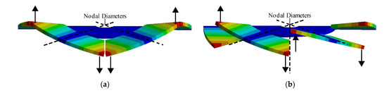
Figure 3.
Torsional modes: (a) Blades without a nodal diameter between them, (b) blades with a nodal diameter between them.
Table 14.
Z = 4: Mode shapes classification.
To classify the mode shapes a nomenclature is proposed. The first term to define is the class of the mode shape, which is given by the number of nodal diameters, counter-phase diameters and nodal circles. This class has the form “(m, n)”. As was studied before, diametrical mode shapes of the disk become two different mode shapes in bladed disks. Then, a number and a letter are added to the mode shape class to classify the mode shapes by type of motion. The letters “B” and “T” indicates a dominant bending and torsion motion of the blades, respectively. The numbers 1, 2, 3… Indicate the number of bending and torsion axes in the blades. An example of the nomenclature application is shown in Table 14.
4. Modal Characteristics of a Kaplan Runner
To complete the above analysis, the mode shapes of bladed disks are compared with the mode shapes of a real Kaplan runner with 4 blades (see Figure 4a). To make this comparison, a modal analysis of a Kaplan rotor is carried out by means of numerical simulation. The geometry of the rotor includes the runner, with its inner control system, (see Figure 4b), the shaft and the generator. An Elastic Support condition with a Support Stiffness of 109 N/mm3 is used. This boundary condition is placed in the thrust bearing location (see Figure 4c). In Table 15, the main dimensions of the rotor, indicated in Figure 4c, are defined as a function of the runner outer diameter Do.
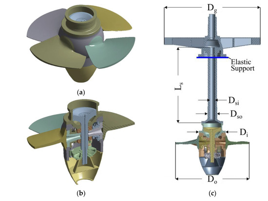
Figure 4.
Kaplan runner model: (a) Runner, (b) Runner section plane, (c) Rotor main dimensions.
Table 15.
Kaplan rotor main dimensions.
For the mesh, 931562 tetrahedral elements are used. The elements have a size of 70 mm in the blades, 30–70 mm in the inner control system, 100 and 120 mm in the hub and the cone, respectively, and 200 mm in the shaft and generator. These element size values were selected after an analysis of the mesh sensitivity was done.
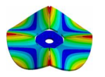
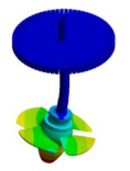
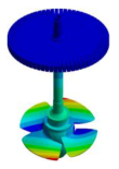
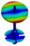
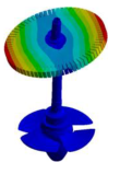
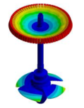
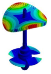
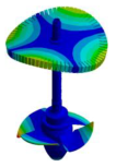
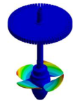
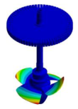
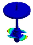
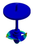
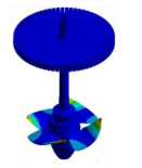
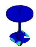
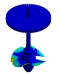
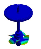
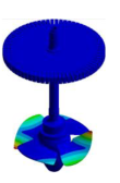
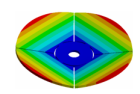
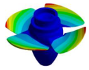
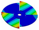
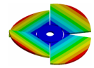
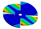
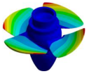
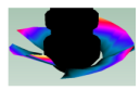
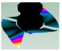
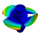
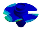
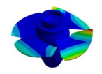
Next, the mode shapes and natural frequencies of the rotor are extracted. Even though the whole rotor is analyzed, its mode shapes are locally defined by its components (runner, shaft and generator). In Table 16, different mode shapes of the rotor are shown. These mode shapes are classified depending on the dominance of the rotor component on the mode shape. In the first row of the table a mode shape dominated by the deflection of the shaft is shown. In this mode shape, the runner moves as a rigid body. In the second row, the mode shapes dominated by the generator are shown. It can be seen that, due to its geometry, its mode shapes are related to disk-like structure mode shapes. Although these are generator-dominated mode shapes, it can be seen that the blades are also excited in global and local mode shapes. Finally, in the third and fourth rows, the ten first mode shapes dominated by the runner are shown. These last mode shapes are the ones studied in this paper.
Table 16.
Mode shapes of the Kaplan rotor.
Runner Mode Shapes and their Classifications
For a better analysis of the runner mode shapes, the shaft and generator of the rotor are not represented. In Table 17, a comparison of mode shapes of the bladed disk and the Kaplan runner is shown. In a general view, the modal characteristics of the bladed disk and the runner are similar. Although three mode shapes of the runner were not found in the bladed disk, most of the mode shapes of the runner match the mode shapes of the bladed disk. Then, the mode shapes of the Kaplan runner can be classified with the same criteria proposed for bladed disks.
Table 17.
Classification of the runner mode shapes.
The unidentified mode shapes are classified as (1,0)1B, (3,0)1T1B and (4,0)1T-1 (see Table 17). In the first unidentified mode shape, 1 nodal diameters is detected. While in the second mode shape 3 nodal diameters are detected. These mode shapes correspond to the class (1,0) and (3,0), respectively. Moreover, it can be noticed that the first mode is dominated by the first bending motion (1B) of the blades. Thus, the first mode is classified as (1,0)1B. The second mode is dominated by a combination of first torsional and first bending motion of the blades. The subclassification 1T1B is assigned to this condition. Later, the second mode is classified as (3,0)1T1B. Finally, in the third unidentified mode shape, 4 nodal diameters are detected. This mode is dominated by the first torsional motion of the blades. Its classification corresponds to the class (4,0)1T. In this case, two mode similar mode shapes (4,0)1T are detected (see Table 17). A script with a number (−1, −2, −3…) is added to the classification in order to make a difference between the modes which have the same class. These numbers are assigned by the extraction order of the mode shape. As this unidentified mode is detected first, “−1” is added to its classification ((4,0)1T−1).
5. Experimental Modal Analysis of a Kaplan Runner
To complete the analysis of the Kaplan runner mode shapes, the theoretical results in previous sections are contrasted with experimental data. The rotor geometry studied in the above section belongs to a real machine, which is experimentally studied in this section. Taking advantage of the fact that the runner of the machine was accessible during a scheduled plant stop, different sensors were installed in the runner and an experimental modal analysis (EMA) was carried out. It is important to remark that the EMA was carried out with the runner attached to the rotor.
5.1. Instrumentation
To carry out the modal analysis, the blades are hit several times at different points with a Dytran 5802A instrumented hammer (Dytran Instruments, Chatsworth, United States of America), which has a sensitivity of 220 μV/N. For the vibration measurements, Kistler 8752A ICPaccelerometers (Kistler, Jonsered, Sweden) with a sensitivity of 100 mV/g are used. Both excitation and response signals are recorded by a Brüel & Kjaer Type 3053-B-120 (Brüel & Kjaer, HBK Company, Virum, Denmark)acquisition system, in the time domain, with a sampling frequency of 16384 samples/s. Finally, the data acquired is processed by means of the commercial software BK Connect (by Brüel & Kjaer).
5.2. Runner Mode Shapes
At each hit point, excitation and response signals are recorded in the time domain. In order to calculate the FRF, the acquired signals have to be converted to the frequency domain. To process these signals, exponential windows of 8 s are used. The spectrums are calculated by using the fast Fourier transform (FFT), with a frequency resolution of 0.125 Hz in every window. The spectrums obtained are averaged and a final averaged spectrum is calculated for each excitation and response signal. Then, the FRF of every point is calculated directly from these processed signals. An experimental mesh which represents the location of every hit point with respect to the others is built-in. Each of the obtained FRF is assigned to each degree of freedom of the experimental mesh shown in Figure 5.
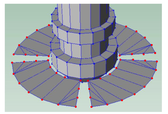
Figure 5.
Experimental mesh and degrees of freedom (red points).
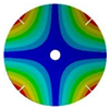
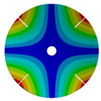
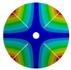
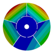
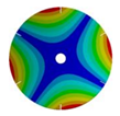
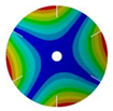
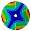
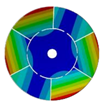
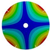
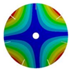
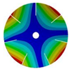
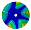
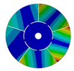
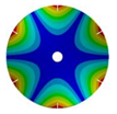
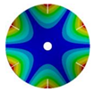
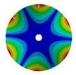
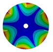
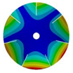
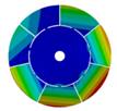
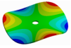
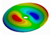
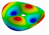
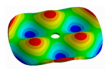
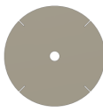
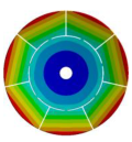
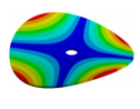
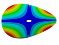
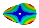
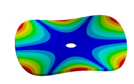
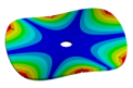
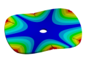
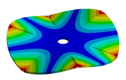
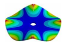
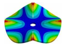
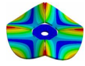
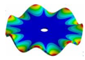
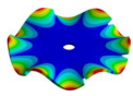
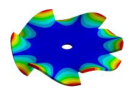
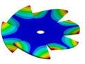
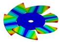
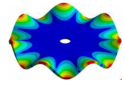
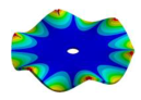
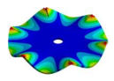
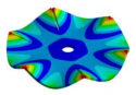
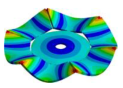
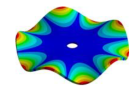
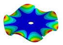
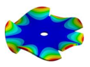
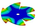
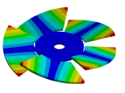
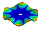
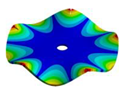
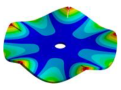
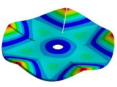
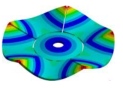
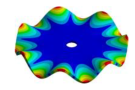
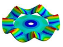
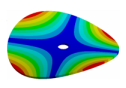
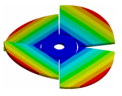
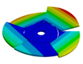
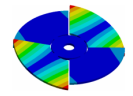
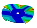
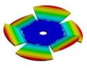
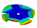
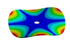
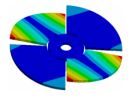
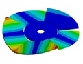
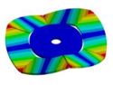
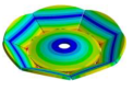
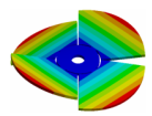
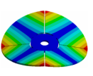
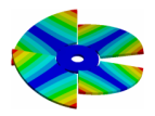
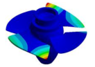
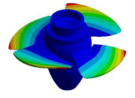
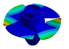
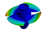
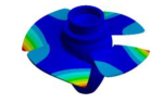
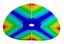
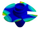
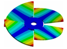
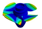
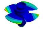
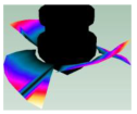
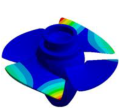
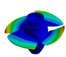
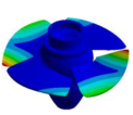
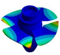
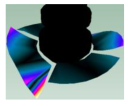
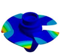
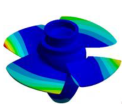
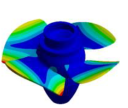
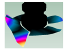
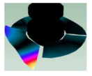
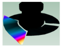
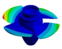
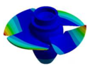
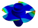
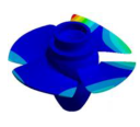
Since the mode shapes of interest are the ones corresponding to the runner, the FRF are analysed from 0 to 100 Hz. Finally, by the peak-picking method, the natural frequencies and the mode shapes of the runner are extracted. An FRF and the mode shapes extracted at each peak, with their respective natural frequencies, are shown in Figure 6.

Figure 6.
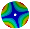
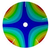
Frequency response function of the Kaplan runner and the mode shapes extracted: (a). 31.625 Hz, (b). 35.875 Hz, (c). 36.625 Hz, (d). 39.375 Hz, (e). 45.625 Hz, (f). 49.625 Hz, (g). 50.375 Hz, (h). 54.125 Hz, (i). 68.750 Hz, (j). 87.625 Hz, (k). 91.500 Hz.
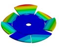
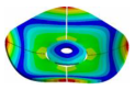
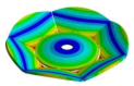
In the shown spectrum, it is possible to see that the mode shapes are dominated by three main blade motions. In the range of 30 to 42 Hz, the mode shapes are dominated by the bending motion of the blades (1B). Then, from 42 to 70 Hz the mode shapes are dominated by the torsional motion of the blades (1T). Finally, the mode shapes between 80 and 100 Hz are dominated by the double torsional motion of the blades (2T). Although in some mode shapes such as Figure 6a,e,f,g, one blade has more amplitude than the other blade, the general motion of all the blades describes a global mode shape. These modes can be classified as shown in Table 18. As seen in this table, not all the mode shapes extracted by FEM are detected in the experimental modal analysis. This can be related to structural damping, which is not considered in the theoretical model. The effect of the damping is that some mode shapes, theoretically extracted, can be merged when their natural frequencies are not well separated.
Table 18.
Runner mode shapes: comparison between numerical and experimental modal analysis.
Finally, the global mode shapes experimentally detected match the FEM model in the mode shapes (1,0), (0,0)1B, (2,0)1B, (2,0)1T and (3,0)1T-1. Therefore, the numerical analysis has been validated with the experimental data.
It is worth saying that a global mode shape that was detected in the EMA was not extracted from the FEM analysis. Following the previously explained criteria, this mode was classified as (3,0)1T.
5.3. Local Mode Shapes
In some cases, such as Figure 6h,j, where the mode shapes are dominated by one blade, the other blades of these mode shapes have no motion. The same effect occurs in Figure 6i, where, just two blades vibrate with the double torsional motion and the counter-side blade of each one does not move (see Table 19). These mode shapes are considered as local mode shapes. The nomenclature proposed to classify these modes is composed by the number of axes of motion (1,2,3….), the type of motion (T for torsion, B for bending), b (for blade) and the identification number of the blades which are excited (1,2,3… < Z) (see Figure 7).
Table 19.
Local mode shapes.
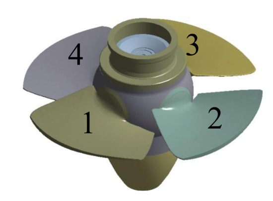
Figure 7.
Identification of the blades.
5.4. Variation of Stiffness
In numerical simulations of Kaplan runners, every blade is considered equal to each other. Nevertheless, in a real runner, slight variations of the stiffness may exist among the blades. These variations can be originated in fabrication processes, surface treatments, by material defects, etc. In order to study the effect of slight variations in the stiffness, the Young modulus of blade 1 (see Figure 7) is reduced by 2%. Then, a numerical modal analysis is carried out with the same mesh characteristics and boundary conditions exposed in Section 4.
The mode shapes extracted after the stiffness variation in blade 1 are shown in Table 20. In this table, it is possible to see that the first mode shape ((0,0)1B at 34.593 Hz) is not affected by the stiffness variation in the blade. In contrast, the second mode shape ((2,0)1B at 37.977 Hz) is affected by this variation in the blade stiffness and some blades have higher amplitude than others. At higher mode shapes, for instance, at 50.498 Hz and 52.712 Hz, the blades vibrate with the same torsion motion but one local mode shape is dominated by the blade 3 and the other one dominated by the blade 4, respectively. It can be concluded that the global mode shapes can be separated in different combinations of local mode shapes due to the variation in the blade stiffness. Even though only one blade stiffness is modified, these numerical results give an idea about the influence of the slight variations of this parameter in the runner blades. It is important to remark that the blade stiffness variation, in a real runner, is distributed in all the blades. Then, different combinations of local mode shapes may be detected.
Table 20.
Mode shapes extracted after a blade stiffness variation.
6. Conclusions
In this study, the mode shapes of Kaplan runners have been thoroughly analyzed and discussed.
To understand the modal characteristics of these bladed structures, four different bladed disks, with 4, 5, 6 and 7 blades, have been studied as simplified models of a Kaplan runner. The mode shapes of bladed disks have been classified according to the number of nodal diameters identified, using the mode shapes of a simple disk as a reference. The mode shapes of a bladed disk model and a real runner geometry have been compared using numerical simulations. Next, the results obtained from the real Kaplan simulation have been validated using experimental data obtained from an experimental modal analysis.
By the tracking and identification of the disk nodal diameters on the bladed disks, it is found that the blade disk mode shapes are dependent on the blade number. On one hand, bladed disks with an even blade number have a uniform deformation distribution in the mode shape when the mode has (k*Z)/2 nodal diameters (with k = 1,2,3… and Z is the blade number). On the other hand, bladed disks with an odd blade number have a uniform deformation distribution, when the mode has k*z nodal diameters. In other cases, the mode shapes match the structure by a non-uniform deformation of the blades. Then, bending and torsional modes of the blades can coexist in a global mode shape, vibrating at different amplitudes.
A classification of the mode shapes of bladed disk has been carried out. The disk mode shapes have been extracted and its nodal diameters have been tracked in the progressive modification of the disk to model a bladed disk. It was found that not only the disk nodal diameters can be seen in the blades but also in the phase shift between the blades. Then, the mode shapes can be classified as disk mode shapes. The equivalent nodal diameters number is obtained by adding the number of nodal diameters which pass through the blades and the diameters which provokes the counter phase motion between the blades.
Using numerical simulation, it has been proved that the bladed disk model with 4 blades and a real Kaplan runner with the same blade number have similar mode shapes. This was validated by comparing the numerical results with the obtained mode shapes from experimental modal analysis. In the experimental results, global and local mode shapes have been identified and classified. Global mode shapes experimentally found are dominated by the first bending (1B) and first torsion (1T) motion of the blades.
In addition, local mode shapes experimentally found, have been investigated by numerical methods. It is found that slight stiffness variations in the blades can affect the global mode shapes of the runner leading to the generation of local mode shapes.
In this paper, a complete description of mode shapes of Kaplan runners and simplified models is given. This information is useful for the reader to understand the influence of parameters, such as the blade number, on the global mode shapes in the design stage of the runner. Moreover, with this information, an estimation of the mode shapes which can be excited, e.g. if the runner is excited by a rotor-stator interaction, can be carried out.
Author Contributions
Writing-original draft preparation, G.M.; Investigation and numerical study of the bladed disk, G.M.; Numerical simulation of the Kaplan rotor, M.E.; Experimental Modal Analysis, A.P. and D.V.; Supervision, C.V. All authors have read and agreed to the published version of the manuscript.
Funding
This work was funded by the National Agency for Research and Development (ANID)/Scholarship Program/DOCTORADO BECAS CHILE/2020–72210054. Furthermore, this research activity is framed within the context of the XFLEX HYDRO project. The project has received funding from the European Union’s Horizon 2020 research and innovation program under grant agreement No 857832.
Institutional Review Board Statement
Not applicable.
Informed Consent Statement
Not applicable.
Data Availability Statement
Not applicable.
Acknowledgments
Alexandre Presas and David Valentín want to acknowledge the Serra Hunter Program from Generalitat de Catalunya. Mònica Egusquiza would like to acknowledge the Margarita Salas program funded by the European Union.
Conflicts of Interest
The authors declare no conflict of interest.
Appendix A. Detailed Geometries of Bladed Disk and Its Transitions
Table A1.
Transition model and final bladed structure with 4,5,6 and 7 blades.
Table A1.
Transition model and final bladed structure with 4,5,6 and 7 blades.
| Z | Transition 1 | Transition 2 | Transition 3 | Final Model |
|---|---|---|---|---|
| 4 | 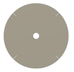 | 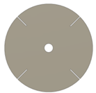 | 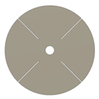 |  |
| 5 | 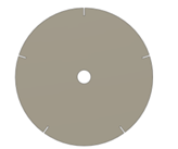 | 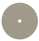 | 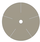 | 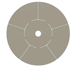 |
| 6 | 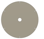 | 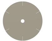 | 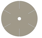 | 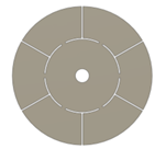 |
| 7 | 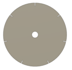 | 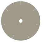 | 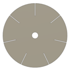 | 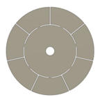 |
Appendix B. Mode (1,0), (2,0) and (3,0) for All Transition Geometries and Bladed Disks
Table A2.
Transition from the disk to the bladed disk at the vibration mode (1,0).
Table A2.
Transition from the disk to the bladed disk at the vibration mode (1,0).
| Z | Transition 1 | Transition 2 | Transition 3 | Final Model |
|---|---|---|---|---|
| 4 |  |  |  |  |
| 167.55 | 166.92 | 150.75 | 104.52 | |
| 5 | 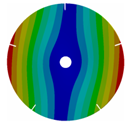 | 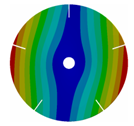 | 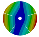 | 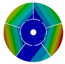 |
| 167.47 | 167.36 | 158.63 | 118.19 | |
| 6 | 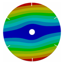 | 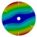 | 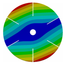 | 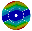 |
| 167.57 | 167.43 | 162.73 | 133.65 | |
| 7 |  | 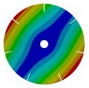 | 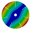 | 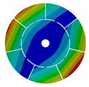 |
| 167.62 | 167.66 | 164.79 | 145.46 |
Table A3.
Transition from the disk to the bladed disk at the modes (2,0).
Table A3.
Transition from the disk to the bladed disk at the modes (2,0).
| Z | Transition 1 | Transition 2 | Transition 3 | Final Model |
|---|---|---|---|---|
| 4 | 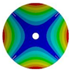 | 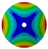 |  | 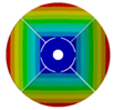 |
| 264.98 Hz | 245.03 Hz | 152.50 Hz | 101.26 Hz | |
 |  |  |  | |
| 266.55 Hz | 254.25 Hz | 216.49 Hz | 144.87 Hz | |
| 5 | 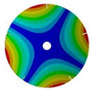 | 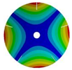 | 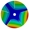 | 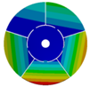 |
| 268.07 Hz | 257.62 Hz | 188.58 Hz | 120.32 Hz | |
 |  |  |  | |
| 268.07 Hz | 257.62 Hz | 188.59 Hz | 120.31 Hz | |
| 6 | 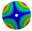 | 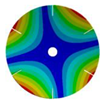 | 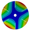 | 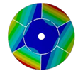 |
| 267.42 Hz | 254.97 Hz | 208.35 Hz | 143.41 Hz | |
 |  |  |  | |
| 267.42 Hz | 254.97 Hz | 208.35 Hz | 143.41 Hz | |
| 7 | 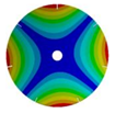 | 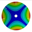 | 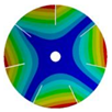 | 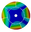 |
| 268.08 Hz | 257.89 Hz | 220.39 Hz | 163.58 Hz | |
 |  |  |  | |
| 268.08 Hz | 257.90 Hz | 220.38 Hz | 163.58 Hz |
Table A4.
Transition from the disk to the bladed disk at the vibration mode (3,0).
Table A4.
Transition from the disk to the bladed disk at the vibration mode (3,0).
| Z | Transition 1 | Transition 2 | Transition 3 | Final Model |
|---|---|---|---|---|
| 4 | 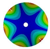 | 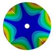 | 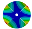 |  |
| 576.89 Hz | 507.55 Hz | 283.68 | 154.12 Hz | |
 |  |  |  | |
| 577.27 Hz | 510.25 Hz | 283.67 Hz | 154.13 Hz | |
| 5 | 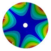 | 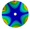 | 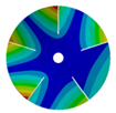 | 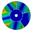 |
| 586.92 Hz | 541.60 Hz | 336.81 Hz | 177.91 Hz | |
 |  |  |  | |
| 586.93 Hz | 541.60 Hz | 336.80 Hz | 177.91 Hz | |
| 6 | 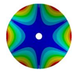 | 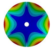 | 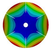 | 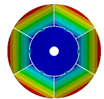 |
| 583.52 Hz | 520.45 Hz | 313.76 Hz | 163.84 Hz | |
 |  |  |  | |
| 583.99 Hz | 539.40 Hz | 430.09 Hz | 224.71 Hz | |
| 7 | 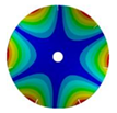 | 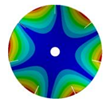 | 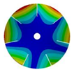 | 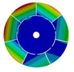 |
| 586.53 Hz | 541.55 Hz | 382.78 Hz | 206.30 Hz | |
 |  |  |  | |
| 586.53 Hz | 541.54 Hz | 382.78 Hz | 206.31 Hz |
References
- IEA. Global Energy Review 2021; IEA: Paris, France, 2021; Available online: https://www.iea.org/reports/global-energy-review-2021 (accessed on 26 June 2022).
- IRENA. Renewable Energy Statistics 2021; The International Renewable Energy Agency: Abu Dhabí, United Arab Emirates, 2021. [Google Scholar]
- Deschênes, C.; Fraser, R.; Fau, J.-P. New trends in turbine modelling and new ways of partnership. In Proceedings of the International Group of Hydraulic Efficiency Measurement (IGHEM), Toronto, ON, Canada, 17–19 July 2002; pp. 1–12. [Google Scholar]
- Valentín, D.; Presas, A.; Valero, C.; Egusquiza, M.; Egusquiza, E. Detection of Hydraulic Phenomena in FrancisTurbines with Different Sensors. Sensors 2019, 19, 4053. [Google Scholar] [CrossRef] [PubMed] [Green Version]
- Egusquiza, E.; Valero, C.; Valentin, D.; Presas, A.; Rodriguez, C.G. Condition monitoring of pump-turbines. New challenges. Meas. J. Int. Meas. Confed. 2015, 67, 151–163. [Google Scholar] [CrossRef] [Green Version]
- Valero, C.; Egusquiza, M.; Egusquiza, E.; Presas, A.; Valentin, D.; Bossio, M. Extension of Operating Range in Pump-Turbines. Influence of Head and Load. Energies 2017, 10, 2178. [Google Scholar] [CrossRef] [Green Version]
- Trivedi, C.; Gandhi, B.; Cervantes, M. Effect of transients on Francis turbine runner life: A review. J. Hydraul. Res. 2013, 51. [Google Scholar] [CrossRef]
- Zhang, M.; Valentín, D.; Valero, C.; Egusquiza, M.; Egusquiza, E. Failure investigation of a Kaplan turbine blade. Eng. Fail. Anal. 2019, 97, 690–700. [Google Scholar] [CrossRef]
- Luo, Y.; Wang, Z.; Zeng, J.; Lin, J. Fatigue of piston rod caused by unsteady, unbalanced, unsynchronized blade torques in a Kaplan turbine. Eng. Fail. Anal. 2010, 17, 192–199. [Google Scholar] [CrossRef]
- Wang, Z.W.; Luo, Y.Y.; Zhou, L.J.; Xiao, R.F.; Peng, G.J. Computation of dynamic stresses in piston rods caused by unsteady hydraulic loads. Eng. Fail. Anal. 2008, 15, 28–37. [Google Scholar] [CrossRef]
- Liang, Q.W.; Rodríguez, C.G.; Egusquiza, E.; Escaler, X.; Avellan, F. Numerical Modal Analysis on a Francis Turbine Runner With Finite Element Method Considering Added Mass Effect. 2005. Available online: https://www.semanticscholar.org/paper/1-Numerical-modal-analysis-on-a-Francis-turbine-Liang-Rodr%C3%ADguez/69fe05340c0ed131fbeb83236ffe56f5633a6154 (accessed on 26 June 2022).
- Rodriguez, C.G.; Egusquiza, E.; Escaler, X.; Liang, Q.W.; Avellan, F. Experimental investigation of added mass effects on a Francis turbine runner in still water. J. Fluids Struct. 2006, 22, 699–712. [Google Scholar] [CrossRef]
- Singhal, R.K.; Guan, W.; Williams, K. Modal analysis of a thick-walled circular cylinder. Mech. Syst. Signal Process. 2002, 16, 141–153. [Google Scholar] [CrossRef]
- Huang, X.X.; Egusquiza, E.; Valero, C.; Presas, A. Dynamic behaviour of pump-turbine runner: From disk to prototype runner. IOP Conf. Ser. Mater. Sci. Eng. 2013, 52, TOPIC 2. [Google Scholar] [CrossRef]
- Presas, A.; Valentin, D.; Egusquiza, E.; Valero, C.; Seidel, U. On the detection of natural frequencies and mode shapes of submerged rotating disk-like structures from the casing. Mech. Syst. Signal Process. 2015, 60, 547–570. [Google Scholar] [CrossRef] [Green Version]
- Valentin, D.; Presas, A.; Egusquiza, E. Influence of Non-Rigid Sufaces on the Dynamic Response of a Submerged and Confined Disk. In Proceedings of the 6th IAHR International Meeting of the Workgroup on Cavitation and Dynamic Problems in Hydraulic Machinery and Systems, Ljubljana, Slovenia, 9–11 September 2015. [Google Scholar]
- Louyot, M.; Nennemann, B.; Monette, C.; Gosselin, F.P. Modal analysis of a spinning disk in a dense fluid as a model for high head hydraulic turbines. J. Fluids Struct. 2019, 94, 102965. [Google Scholar] [CrossRef] [Green Version]
- Muhsen, A.A.; Al-Malik, A.A.R.; Attiya, B.H.; Al-Hardanee, O.F.; Abdalazize, K.A. Modal analysis of Kaplan turbine in Haditha hydropower plant using ANSYS and SolidWorks. IOP Conf. Ser. Mater. Sci. Eng. 2021, 1105, 012056. [Google Scholar] [CrossRef]
- Vialle, J.-P.; Lowys, P.-Y.; Dompierre, F.; Sabourin, M. Prediction of natural frequencies in water-Application to a Kaplan runner. In Proceedings of the HydroVision 2008, Sacremento, CA, USA, 14–18 July 2008; p. 252. [Google Scholar]
- Zhang, M.; Chen, Q.G. Numerical Model on the Dynamic Behavior of a Prototype Kaplan Turbine Runner. Math. Probl. Eng. 2021, 2021, 4421340. [Google Scholar] [CrossRef]
- Zhang, M. On the Changes in Dynamic Behavior Produced by the Hydraulic Turbine Runner Damage. Tesi Doctoral, UPC, Departament de Mecànica de Fluids, Barcelona. 2019. Available online: http://hdl.handle.net/2117/166975 (accessed on 26 June 2022).
- Cao, J.; Luo, Y.; Presas, A.; Ahn, S.H.; Wang, Z.; Huang, X.; Liu, Y. Influence of rotation on the modal characteristics of a bulb turbine unit rotor. Renew. Energy 2022, 187, 887–895. [Google Scholar] [CrossRef]
- Modal Analysis Theory. In Noise and Vibration Analysis; John Wiley & Sons Ltd.: Hoboken, NJ, USA, 2011; pp. 119–146. [CrossRef]
- Heylen, W.; Lammens, S.; Sas, P. Modal Analysis Theory and Testing; Katholieke Universiteit Leuven: Leuven, Belgium, 2007. [Google Scholar]
- Southwell, R.V. On the Free Transverse Vibrations of a Uniform Circular Disc Clamped at Its Centre; and on the Effects of Rotation. Proc. R. Soc. London. Ser. A Contain. Pap. A Math. Phys. Character 1922, 101, 133–153. [Google Scholar]
- Leissa, A.W. Vibration of Plates; Scientific and Technical Information Division, National Aeronautics and Space Administration: Washington, DC, USA, 1969. [Google Scholar]
- Braun, S.; Diego, S.; Francisco, S.; York, N.; London, B.; Tokyo, S. Encyclopedia of Vibration; Academic Press: Cambridge, MA, USA, 2001. [Google Scholar] [CrossRef]
- Presas, A.; Valentin, D.; Valero, C.; Egusquiza, M.; Egusquiza, E. Experimental measurements of the natural frequencies and mode shapes of rotating disk-blades-disk assemblies from the stationary frame. Appl. Sci. 2019, 9, 3864. [Google Scholar] [CrossRef] [Green Version]
- Berger, S.; Aubry, E.; Marquet, F.; Thomann, G. Experimental Modal Shape Identification Of A Rotating Asymmetric Disk Subjected To Multiple-Frequency Excitatoin: Use Of Finite Impulse Response (FIR) Filters. Soc. Exp. Mech. 2003, 27, 44–48. [Google Scholar] [CrossRef]
- Oldac, O.; Tufekci, M.; Genel, O.E.; Tufekci, E. Free Bending Vibrations of Rotating Disks With A Concentric Hole. Int. J. Technol. Eng. Stud. 2017, 3, 253–263. [Google Scholar] [CrossRef]
- Zhao, J.; Zhang, Y.; Jiang, B. A Study on Mode Shape and Natural Frequency of Rotating Flexible Cracked Annular Thin Disk. Shock Vibrat. 2021, 2021, 6533487. [Google Scholar] [CrossRef]
- Blevins, R.D. Formulas for Natural Frequency and Mode Shape/Robert D. Blevins; Van Nostrand Reinhold Co.: New York, NY, USA, 1979. [Google Scholar]


Publisher’s Note: MDPI stays neutral with regard to jurisdictional claims in published maps and institutional affiliations. |
© 2022 by the authors. Licensee MDPI, Basel, Switzerland. This article is an open access article distributed under the terms and conditions of the Creative Commons Attribution (CC BY) license (https://creativecommons.org/licenses/by/4.0/).