Depth Estimation for Egocentric Rehabilitation Monitoring Using Deep Learning Algorithms

Abstract

Upper limb impairment is one of the most common problems for people with neurological disabilities, affecting their activity, quality of life (QOL), and independence. Objective assessment of upper limb performance is a promising way to help patients with neurological upper limb disorders. By using wearable sensors, such as an egocentric camera, it is possible to monitor and objectively assess patients’ actual performance in activities of daily life (ADLs). We analyzed the possibility of using Deep Learning models for depth estimation based on a single RGB image to allow the monitoring of patients with 2D (RGB) cameras. We conducted experiments placing objects at different distances from the camera and varying the lighting conditions to evaluate the performance of the depth estimation provided by two deep learning models (MiDaS & Alhashim). Finally, we integrated the best performing model for depth-estimation (MiDaS) with other Deep Learning models for hand (MediaPipe) and object detection (YOLO) and evaluated the system in a task of hand-object interaction. Our tests showed that our final system has a 78% performance in detecting interactions, while the reference performance using a 3D (depth) camera is 84%.

1. Introduction

Upper limb impairment is one of the most common problems for people with neurological disabilities. If affects the activity, performance, quality of life (QOL), and independence of the person [1]. There are different reasons why a patient may experience upper limb impairment. Stroke is the most common cause of long-term disability worldwide and is known to cause various impairments such as weakness or cognitive deficits in body functions. Each year, 13 million new strokes occur, and nearly 75% of stroke victims suffer from various degrees of functional impairment [2,3,4]. Moreover, it is estimated that by 2030, approximately 973 million adults worldwide will be 65 years of age or older [5]. As people age, more and more are affected by limb impairments and neurodegenerative diseases that cause them difficulties in activities of daily life (ADLs) [1,6].

People who have suffered an accident or stroke must undergo a rehabilitation process to relearn skills that have been suddenly lost due to damage to part of the brain. As part of the rehabilitation process, occupational therapy aims to improve people’s ability to perform activities they need to do (self-care and work) or want to do (e.g., leisure) [7]. Rehabilitation may initially take place in a specialized rehabilitation unit in the hospital before continuing in day rehabilitation centers or at home. Unfortunately, it has been found that patients respond very differently to interventions aimed at restoring upper limb function and that nowadays there are no standard means to objectively monitor and better understand the rehabilitation process [8,9,10]. Objective assessment of limb movement limitations is a promising way to help patients with neurological upper limb disorders. To objectively assess patients’ performance in activities and understanding the impact of intervention, it is first necessary to record what tasks they perform in activities of daily living and during occupational therapies. Therefore, an automatic logging application that provides the interaction of the hand with the environment based on data from an egocentric camera will facilitate the assessment and lead to better rehabilitation process.

ADLs monitoring patient requires a use of 3D (depth) cameras, such as active cameras with time-of-flight sensors, which measure the time it takes for a light pulse to travel from the camera to the object and back again; or stereo-vision cameras, which allow the camera to simulate human binocular vision, giving it the ability to perceive depth.

Consequently, the depth map of the scene provides depth data to any given point in a scene. Accuracy of depth information in active cameras compared to stereo vision cameras is higher [11]. However, using 3D (depth) cameras is associated with some challenges: they are more expensive compared to normal 2D cameras, have a smaller field of view (FOV), are bulky, and require an external battery and memory. Using normal 2D (RGB) cameras, it is possible to only infer the distance of objects in a plane, but not in the 3D space [12].

Depth estimation based on a single image is a prominent task in understanding and reconstructing scenes [13,14,15,16]. Thanks to the recent development of Deep Learning models, depth estimation can be done using deep neural networks trained in a fully supervised manner with the RGB images as input and the estimated depth as output. The accuracy of reconstructing 2D to 3D images has steadily increased in recent years, although the quality and resolution of these estimated depth maps is still poor and often results in a fuzzy approximation at low resolution [13].

Previous studies have shown that 3D (depth) cameras are used in clinical settings, e.g., to prevent/detect falls in the elderly [17,18,19] and to detect activities of daily living [20]. Most applications use a third view and multiple cameras rather than a single and egocentric view. In their study, Zhang et al. proposed a framework to detect 13 ADLs to increase the independence of the elderly and improve the quality of life at home using third-vision RGB-D cameras [20]. In another work, Jalal and colleagues demonstrated lifelong human activity recognition (HAR) using indoor depth video. They used a single camera system with third vision and trained Hidden Markov Models (HMMs) for HAR using the body’s joint information [21].

To the best of the author’s knowledge, monitoring of patients with 2D (RGB) cameras has not been used by taking advantage of deep learning models for depth estimation.

We are currently working on the development of a wearable system that integrates an egocentric camera (first-person perspective) to provide objective information particularly interested in monitoring upper limb rehabilitation, such as the objects the patient can interact with, the type of activities the patient can successfully perform, etc. The camera should capture the objects in the environment and the patient’s hands during ADLs, such as during occupational therapy. This requires three-dimensional data to be captured so that the objects in the scene can be accurately located. Given the aforementioned drawbacks of 3D (depth) cameras, we use deep learning models to reconstruct the depth map from 2D (RGB) images.

Considering this study and its final goal, some considerations must be made to choose the right Deep Learning model for our application. The robustness of the method with respect to different conditions, such as the ability to process a large amount of data, since our final goal is an application with embedded systems to monitor ADLs over a period of time (e.g., 2 months), resulting in a large amount of data, force us to choose a model with high accuracy and fast computational effort. More importantly, another condition to consider is lighting, since the environment is not controlled during the acquisition of patients’ ADLs.

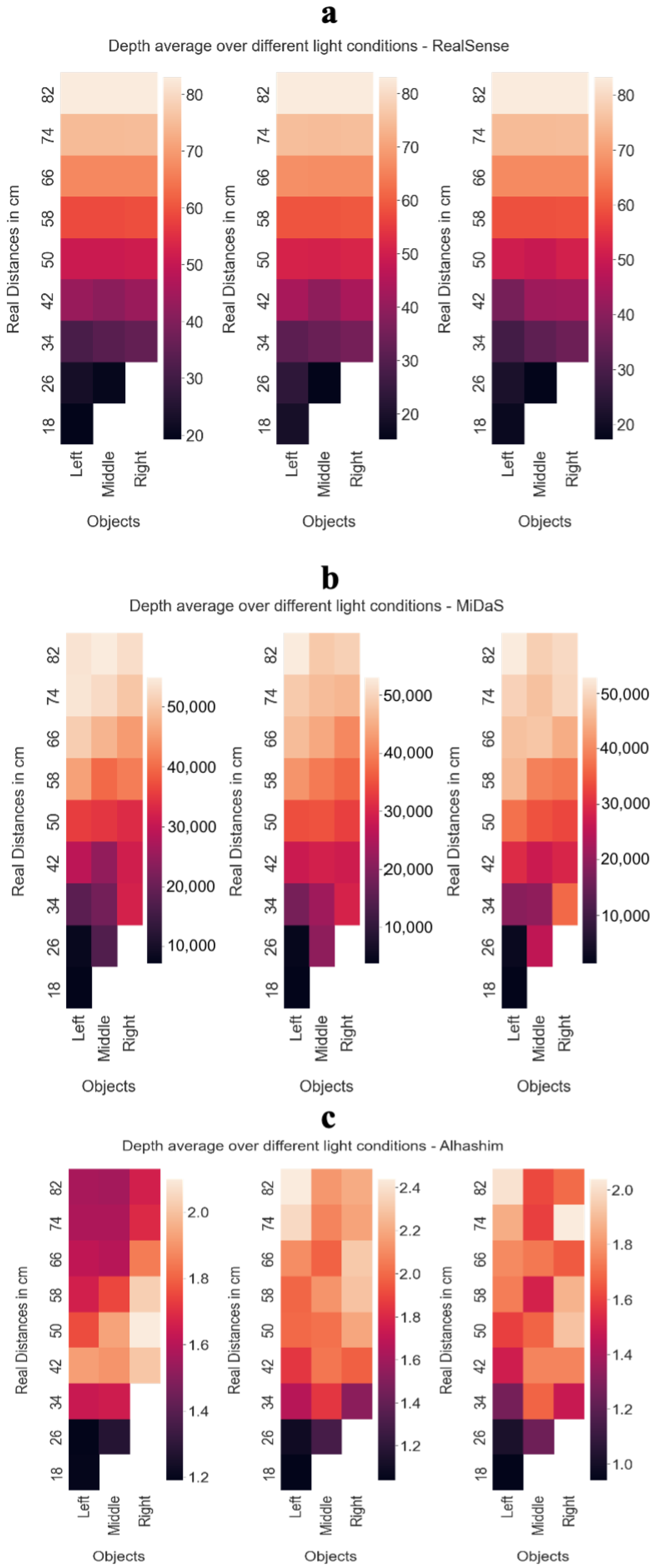
Accordingly, this work focuses on comparing the estimated depth difference based on two different depth estimation methods and a 3D (depth) camera under different lighting conditions: MiDaS (Mixing Datasets for Zero-shot Cross-dataset Transfer [22]), High Quality Monocular Depth Estimation via Transfer Learning (based on Alhashim et al. [13]), and Intel RealSense D435i 3D (depth) camera. We used MiDaS and Alhashim pre-trained models for our comparison to account for extreme cases, as we do not have enough data sets for fine-tuning. The models were already trained on large, diverse datasets with different range of depths, including indoor and outdoor environments, all of which are privileged in our case, to have a generalized model.

The following parts of the article are organised as follows. In Section 2, we explain the depth estimation based on deep learning models in more detail. In Section 3, we describe our experimental setups, dataset preparation and outlines the methodology behind the work. In Section 4, we present results of the different depth estimation methods and, more importantly, examine the consistency of the depth difference between objects in each method. We also briefly inspect the effects of light on depth estimation. The final part of the Section 4 devotes to the application of depth estimation in hand-object interaction. Later, Section 5 dedicates to a discussion of results. Finally, in Section 6, we draw our conclusions.

2. Deep Learning for Depth Estimation

The depth information of the surrounding is useful to understand the 3D scene. The traditional approach to provide depth information is to use 3D (depth) cameras that provide depth information. However, nowadays, commercially available 3D (depth) cameras have some disadvantages as mentioned before. Therefore, this has led us to search for and explore depth estimation possibilities with 2D (RGB) cameras. To select the appropriate model for our application, some considerations must be made, such as the loss function of deep learning models, which can have a significant impact on the training speed and overall performance of depth estimation [13]. Moreover, fast computation of the image is also crucial for the applicability of the methods, since in our final application with embedded systems we have to deal with a large amount of daily recording data for each patient. In addition, the robustness of the method to different conditions, such as light is important since the environment is not controlled during the acquisition.

Therefore, a flexible loss function was proposed based on recent literature and the robustness and generality of the models were evaluated by zero-shot cross-dataset transfer [22]. Furthermore, providing high quality depth maps that more accurately capture object boundaries plays an important role in selecting the model for depth estimation. Therefore, two current candidates were applied to our dataset to verify their compatibility and test their robustness.

The first candidate is a model whose robustness and generality was evaluated using zero-shot cross-dataset transfer (MiDaS), i.e., authors evaluated datasets that were not seen during training. The experiments confirm that mixing data from complementary sources significantly improves monocular depth estimation. They intentionally merged datasets with different properties and biases to scale depth in different environments and guide it through deep networks. Ranftl et al. have presented a flexible loss function and a principled strategy for mixing datasets [22]. They also have shown that training models for monocular depth estimation on different datasets is challenging due to the differences in ground truth. Therefore, they needed to develop a loss function that is flexible enough to work with different data sources. Hence, they compared different loss functions and their results and evaluate the impact of encoder architectures such as ResNet-50 encoder, ResNet-101, ResNeXt-101 and so on. Finally, they proposed a flexible loss function and a principled shuffling strategy for monocular depth estimation.

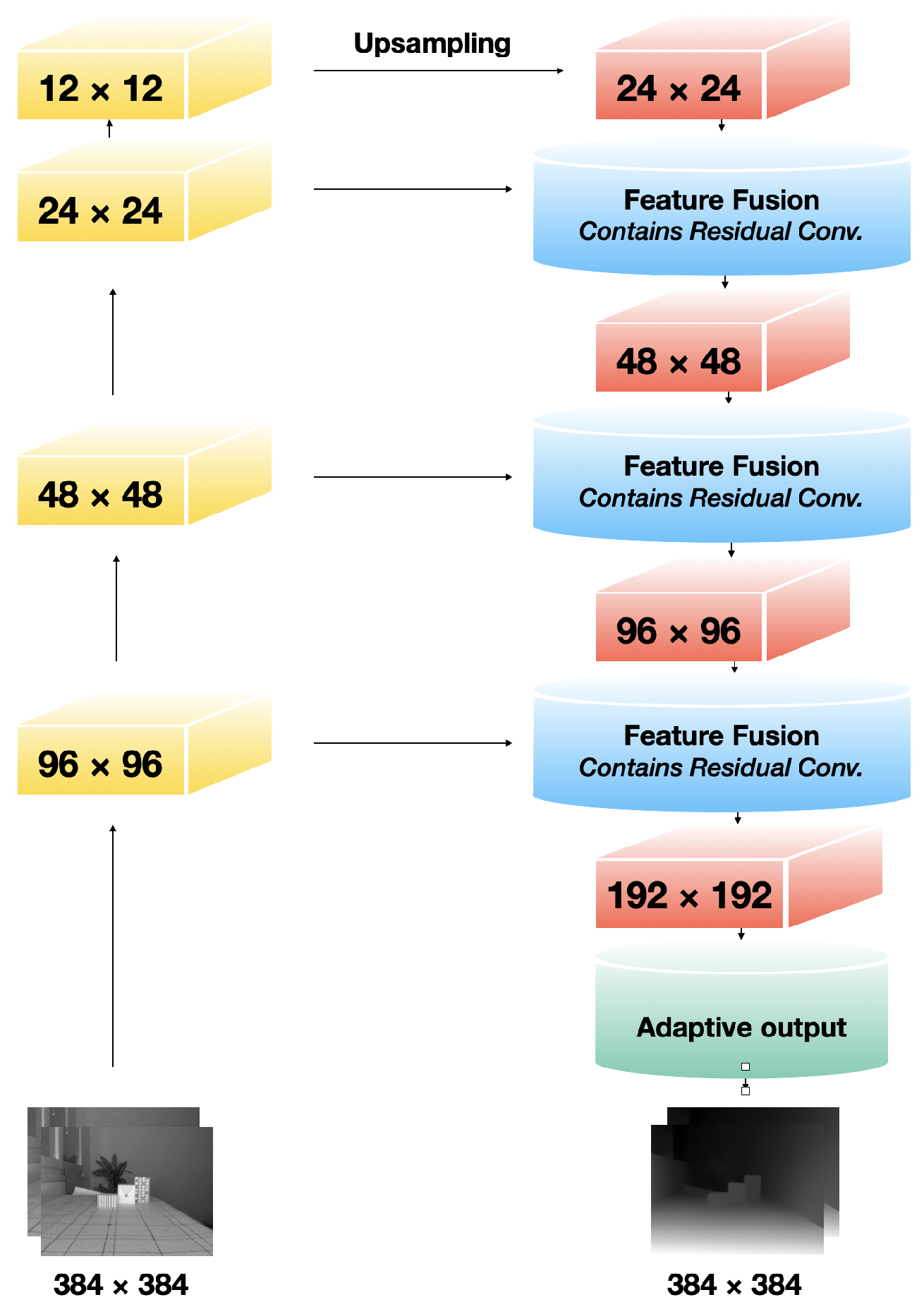
Figure 1 shows the network architecture proposed by K. Xian et al. [23] used in the MiDaS method as their base architecture. Their network is based on a feed-forward ResNet [22]. To obtain more accurate predictions, they used a progressive refinement strategy to fuse multi-scale features. They used a residual convolution module and up-sampling to fuse the features. At the end, there is an adaptive convolution module that adjusts the channels of the feature maps and provides the final output. Ranftl et al. used K. Xian et al. ResNet-based and multi-scale architecture to predict single-image depth. For the encoder part they initialized it with the pretrained ImageNet weights, and for other layers they initialized weights randomly using Adam.

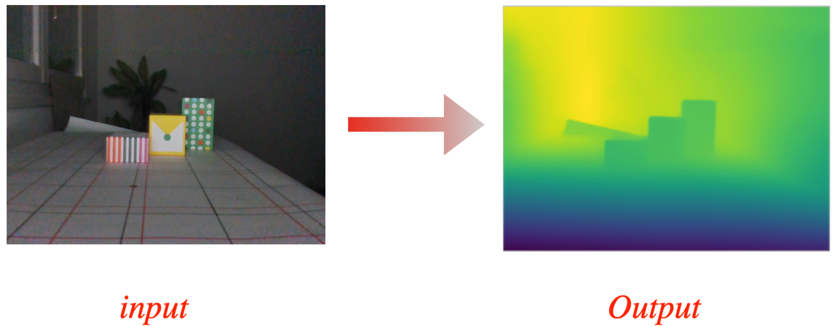
Figure 2 shows the result of depth estimation based on the MiDaS method for a single RGB image from our dataset.

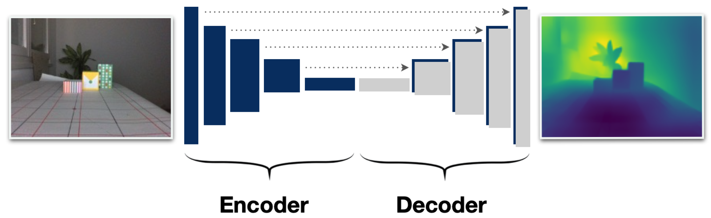
The second method we chose is the work of Alhashim et al., which proposes a convolutional neural network to compute a high-resolution depth map for a single RGB image using transfer learning [13]. They have shown that the standard encoder-decoder method shows in Figure 3 can extract a high-resolution depth map that outperforms more complex training algorithms in terms of accuracy and visual quality. We chose this method since it is computationally cheap. They use a straightforward encoder-decoder architecture. The encoder part is a pretrained DenseNet-169 model. The decoder consists of 2× bilinear up-sampling step followed by two standard convolutional layers [13]. The key factor in their proposed model is the use of encoders that do not greatly reduce the spatial resolution of the input images.

The output depth data of each method for RGB images have different resolutions. Therefore, we modified the structure of the networks in MiDaS and Alhashim to be compatible with the inputs and provide the same resolution in the output. A detailed explanation can be found in Section 3. Also, to obtain a unit for the estimated depth, we need to perform the calibration for each model by comparing it to the ground truth. However, since we are interested in the difference in depth and not necessarily the absolute values, we did not perform complex calculations to create equations for assigning estimated values to cm. Therefore, what is important to us is the change in difference of depth for each model separately, even there is no relative unit to cm for the estimations.

3. Materials and Methods

3.1. Experiment Setup A

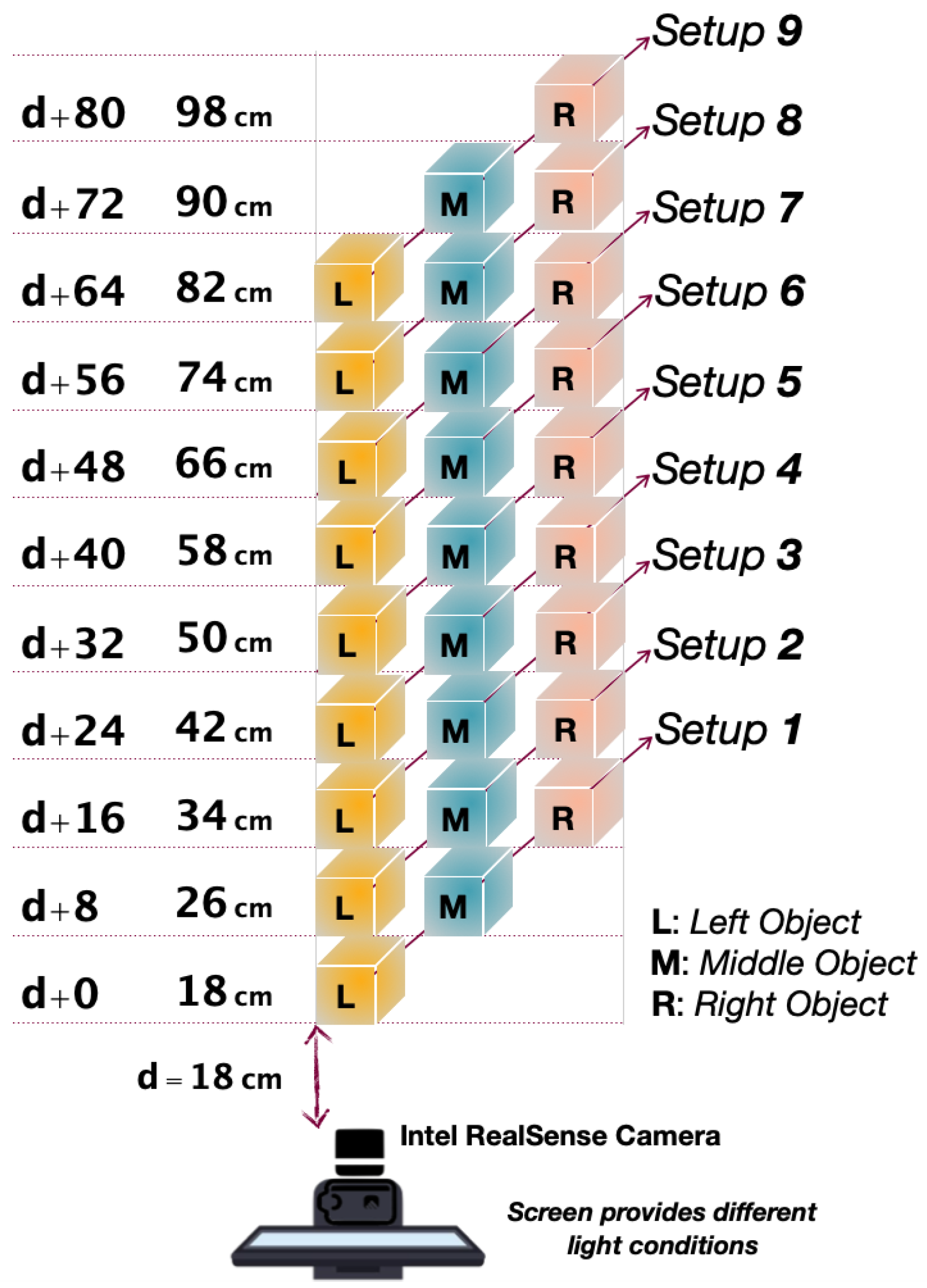
We conducted an experiment under different lighting conditions to capture RGB-Depth images of the scene with objects at different distances from the camera. We designed a configuration showed in Figure 4 and collected data. The back of the camera was in front of the screen, which provides different lighting conditions (Figure 4). The camera used in these experiments was the Intel RealSense D435i, which uses an infrared (IR) projector to provide depth data of the scene and copes with the requirements of our application.

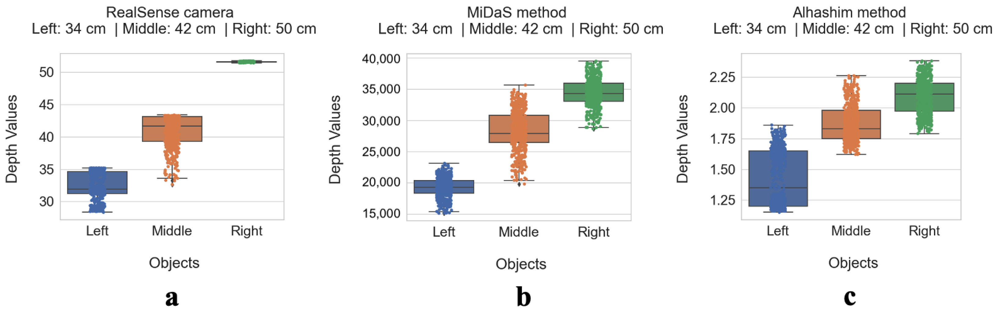
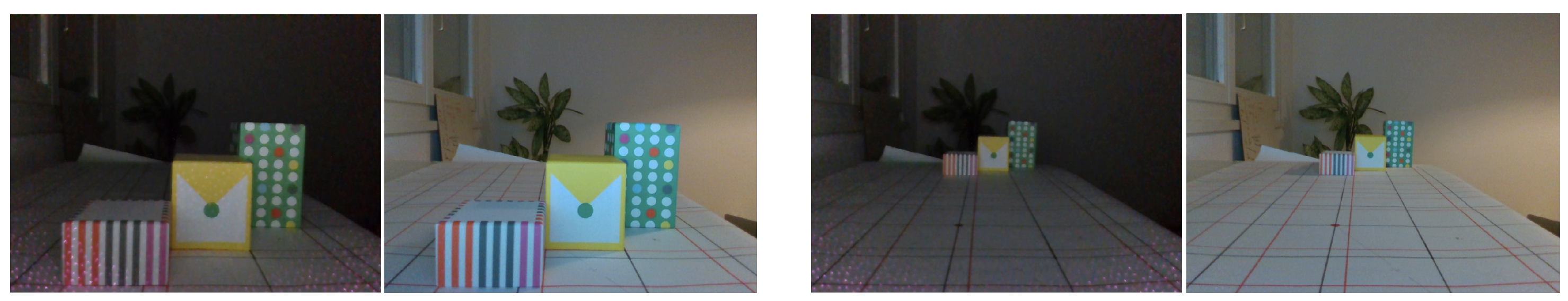
In this experiment, there are 9 configurations in which the objects are positioned at different distances from the camera. This is shown in Figure 4, where the initial distance d is equal to 18 cm. Three objects (L:Left, M: Middle, R: Right) were positioned in each configuration in diagonal order with a horizontal distance of 8 cm between them. Images have been captured for each 9 configurations under different lighting conditions as can be seen in the Figure 5. We were able to achieve the different lighting conditions with a screen behind the camera (Figure 4) where we could automatically increase the brightness by 15 units each time and captured 30 frames of the scene in front.

In the next step, we changed the distances of the objects from the camera (8 cm further from the camera each time) and run the program again to capture another set of images under different lighting conditions. The lighting conditions start at “L-0” (L stands for Lighting), which means there is no light in the scene, and then the brightness increases to the maximum lighting condition (“L-17”). So there are 18 lighting conditions in total: “L-0”, “L-1”, “L-2”, …, “L-16”, “L-17” and 9 configurations. In each setup the 3 objects (Left, Middle and Right) are at a certain distances from the camera, with a 8 cm difference of distance from each other, as shown in Figure 4.

We collected RGB images and depth data using the RealSense D435i camera to create 3 datasets. One is dedicated to the RealSense dataset, which is a kind of off the shelf since it contains depth data based on the proprietary depth sensor IR. The second dataset is based on the MiDaS depth estimation method and the third dataset is dedicated exclusively to the depth estimation method of Alhashim. These last two methods use deep learning to estimate depth based on RGB images. The resolution of the RGB images captured by the Intel RealSense D435i camera is 640 × 480 with a sampling frequency of 30 frames per second.

The Intel RealSense camera provides depth data at the same size as the RGB image, with each pixel having a depth value. The outputs of the Alhashim and MiDaS methods also provide depth data, each in a different range of values.

For MiDaS, the input resolution for the evaluation was adjusted so that the larger axis corresponds to 384 pixels, while the smaller axis was adjusted to a multiple of 32 pixels (a limitation imposed by the encoder), keeping the aspect ratio as close as possible to the original aspect ratio. Thus, for our collected data, the input resolution was 640 × 480, so we had to adjust the encoder to be compatible.

In addition, the architecture of the encoder in Alhsahim expects the image size to be divisible by 32. During testing, the input image was first scaled to the expected resolution, and then the output depth image of 624 × 192 was extrapolated to the original input resolution. The final output was calculated by taking the average of the prediction of an image and the prediction of its mirror image. Therefore, we had to adapt the encoder to accept an input image with a resolution of 640 × 480 and produce an output image with the same resolution of the input data.

Thus, the output depth data of each method for RGB images have the same resolution, which is necessary for comparison.

Outlier Removal—Experiment A Setup

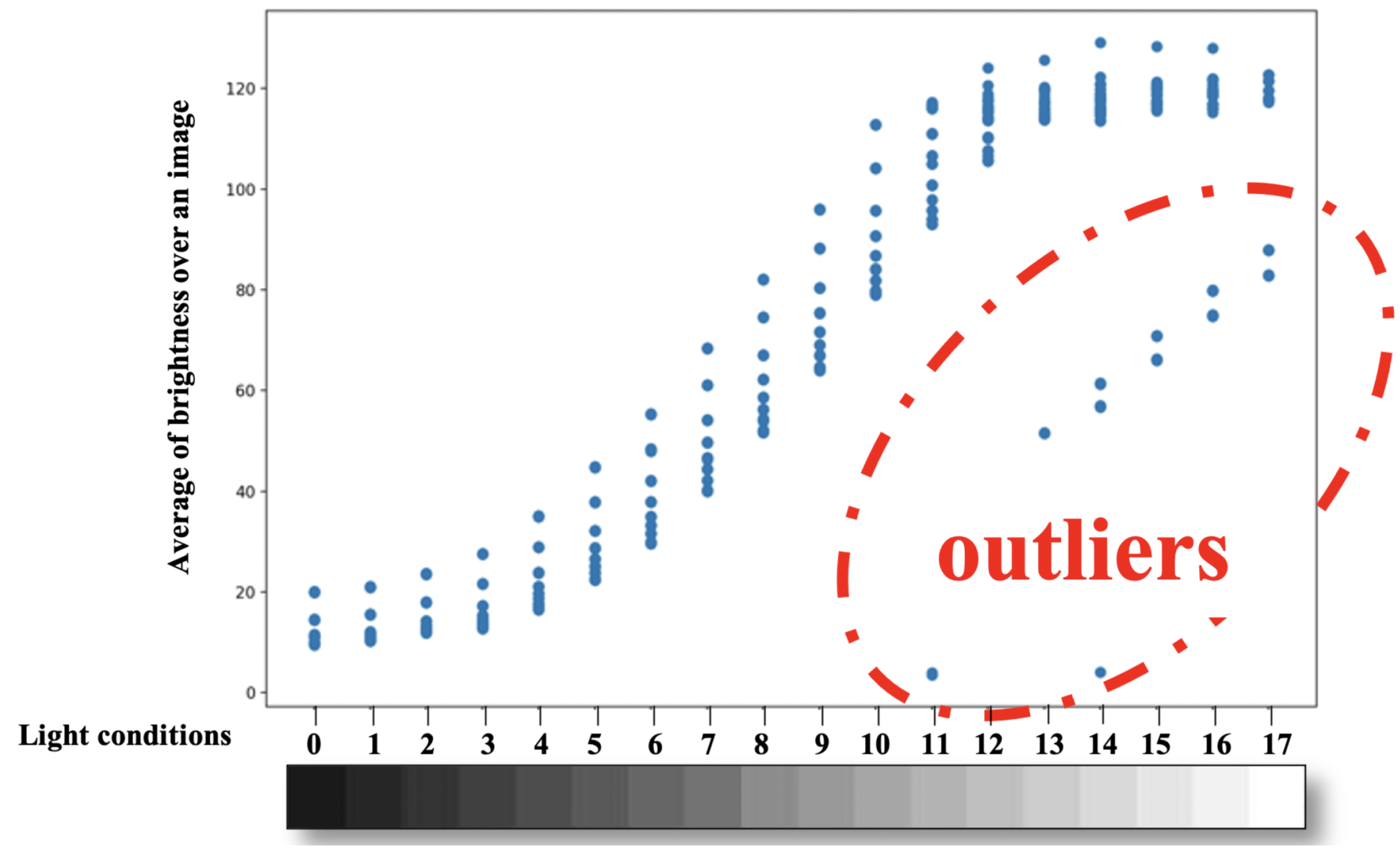
To remove outliers from the datsets collected based on the experimental design A, we visually indicate outliers in Figure 6 by plotting the average of the brightness across all pixels of each image in the direction of the illumination conditions. In Figure 6, the images that do not match their labels are identifiable because the labels of the illumination conditions increase with increasing brightness, but this is not the case for the outlier points. Therefore, we eliminated images whose averaged brightness is below the mode of the values at the same illumination conditions with a threshold of 25 and cleaned the datasets of errors that could be due to the camera or unintended changes in ambient illumination.

3.2. Experiment Setup B

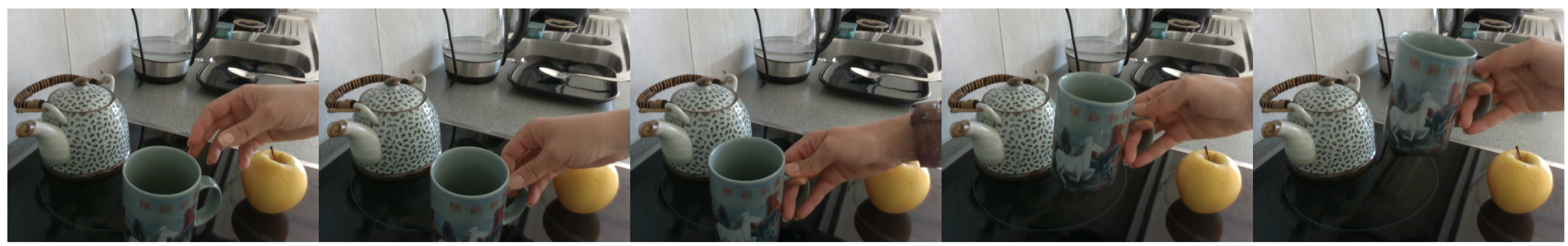
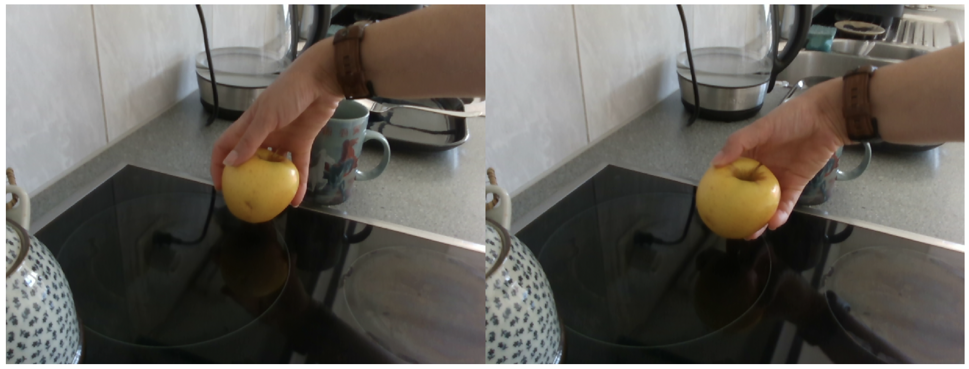
We conducted a simple experiment in which we performed 100 interactions of the hand with objects in different situations, in the office, at home, and in the kitchen, as different locations convey different lighting conditions and the arrangement of objects in the scene. We recorded different videos containing hand reaching, grasping and interaction of the hand with the objects on a table at different distances, as shown in Figure 7 as an example. We recorded our data which contains more than 6000 frames from the egocentric view with similar internal parameters of the camera as we recorded with the Intel RealSense camera in this study. For example, the resolution of the RGB images recorded by the Intel RealSense D435i camera is 640 × 480 and the sampling frequency is 30 frames per second. Similar to the capturing in Section 3.1, there are two images, an RGB image and a depth image as a reference, captured by Intel RealSense camera.

3.3. Dataset Preparation—Experiment A

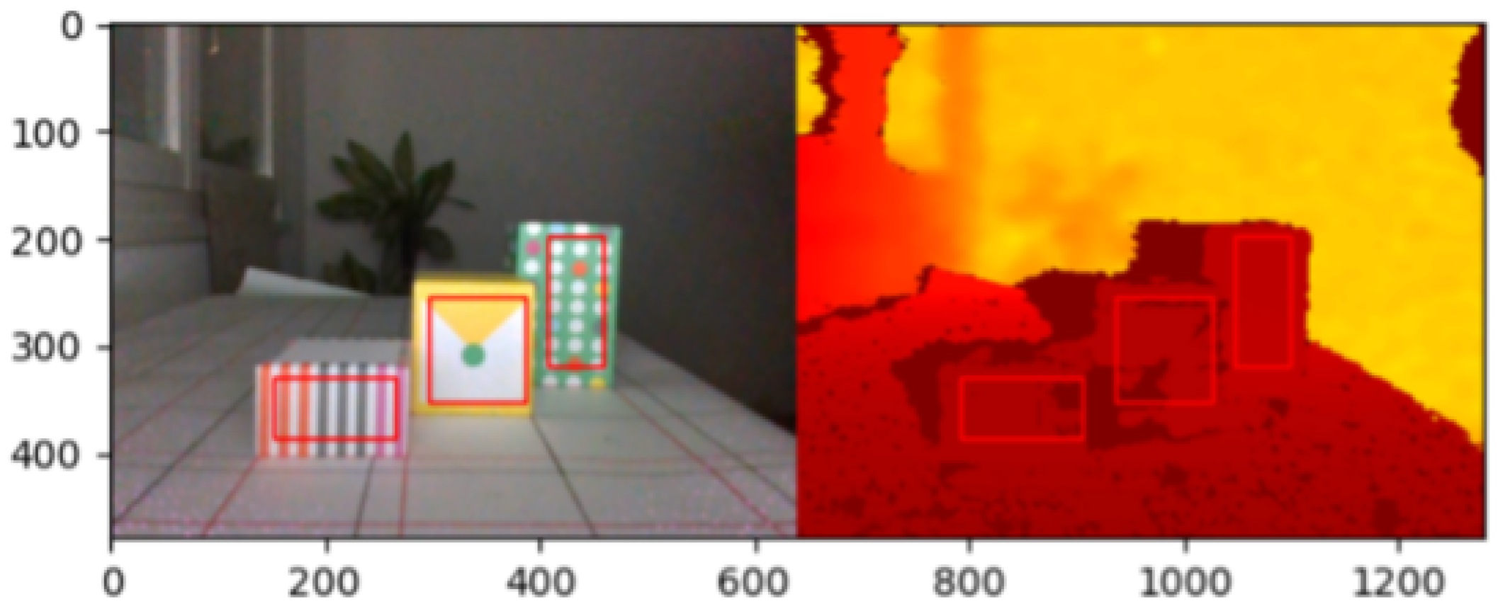
Preparing the dataset is an important step before analysis to remove outliers and refine the datasets. There are “18” lighting conditions. So for each scene there are 18 observations. To increase the accuracy of the measurement, the camera took 30 images for each scene and each lighting condition. Therefore, in each scene there are 540 observations for an object at a certain distance from the camera. The main goal is also to provide a value for each object as a depth representation. To achieve this, we averaged over all pixels within a rectangular boundary for each object (Figure 8).

At the end, there are a total of 3 (objects) × 3 (methods for capturing depth values) × 18 (lighting conditions) × 30 (images for each scene) × 9 (setups) = 43,740 observations.

After collecting the dataset, we must exclude outliers so as not to compromise the analysis. The technique we used to remove outliers from our data frames is based on a correlation between lighting conditions and the average of brightness over an RGB image. Image brightness was calculated for averaging all pixels within a rectangular boundary in an image for R, G, and B, and then averaged to determine the total brightness of a 2D image. We then plotted the total brightness of a 2D image as a function of lighting conditions. To identify outliers, we remove images whose illumination labels do not follow the corresponding line for brightness.

After filtering out the data from outliers, the data were averaged over 30 images of each scene within each light condition by each object. Thus, we obtained one representative for all 30 observations of each object, for a given distance from the camera at a given lighting condition.

3.4. Dataset Preparation—Experiment B

In this experiment, we recorded videos using the Intel RealSense D435i. Therefore, we need to extract the RGB and depth data captured by the camera. After that, no further preparation is required as we will apply our hand-object interaction detection algorithm to detect the interactions.

3.5. Methodology: Hand-Object Interaction Detection

In order to evaluate the usefulness of the depth estimation algorithms in a more realistic setup, we proceeded to use MiDaS for depth estimation in a task where the objective is to detect hand-object interactions based on, Section 3.4 (setup experiment B). We estimated Depth using the MiDaS Deep Learning model from the 2D RGB images to proceed with our analysis. Later, all recorded data were labelled for interactions, such as hand-cup and hand-apple. Therefore, the successes of interaction detection were measured by the type of depth data used by the algorithm. To determine the reliability of depth estimation by MiDaS and compare it with the results of RealSense, we used other Deep Learning models to detect the hand (MediaPipe [24]) and the objects (YOLOv3 [25]). MediaPipe detects 21 3D landmarks and YOLO provides a list of detected objects and the position of bounding boxes indicating their position in the scene. Therefore, in each frame, we compared the interaction between hand and object and check the two below criteria to report an interaction. Since we wanted to keep the analysis simple, we limited ourselves to two criteria, namely the difference in depth between the hand and the object and the difference in pixels in the 2D image. To simplify the measurement of depth, we average over the depth values of the pixels of a region smaller than the detected object (see Figure 8). So, we resized the bounding rectangle and created a smaller rectangle over the surface of the detected object and then average over the depth values of the pixels within the smaller rectangle. For the hand, we also selected three landmarks, drew a bounding rectangle over them, and averaged over the rectangular surface of the hand.

Therefore, in each frame there are the results of hand and object detection, as well as the results of the depth difference between the hand and the object, and the pixel difference in the RGB image between the hand and the object. To decide which image is showing the interaction between the hand and an object, we set a threshold value for the depth difference in the RealSense system and also a different value for the threshold in the MiDaS system because they have different units. However, we chose the same value for the pixel difference because the RGB images are used in both systems are the same. We computed the precision, F1-score and sensitivity to compare the performance of a system using MiDaS and RealSense as our reference.

3.6. Statistical Analysis

3.6.1. Statistical Analysis on Depth Estimation

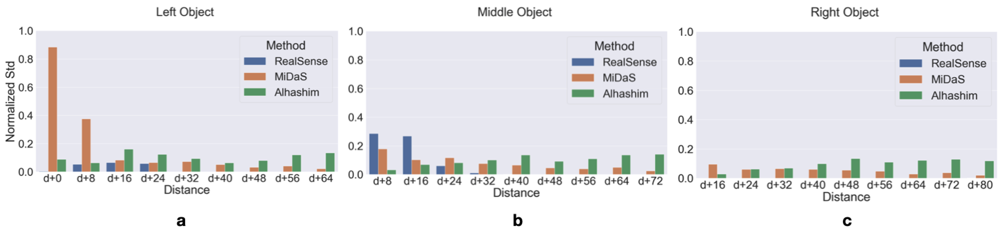
To quantitatively measure the dispersion of depth estimation by each method, we calculated the dispersion based on the normalized standard deviation. We selected the maximum normalized standard deviation across all objects through different distances and lighting conditions to measure the maximum standard deviation corresponding to a distance in each method. Thus, the standard deviation is measured by multiplying the maximum normalized standard deviation by a distance.

3.6.2. Statistical Analysis on Depth Difference Estimation

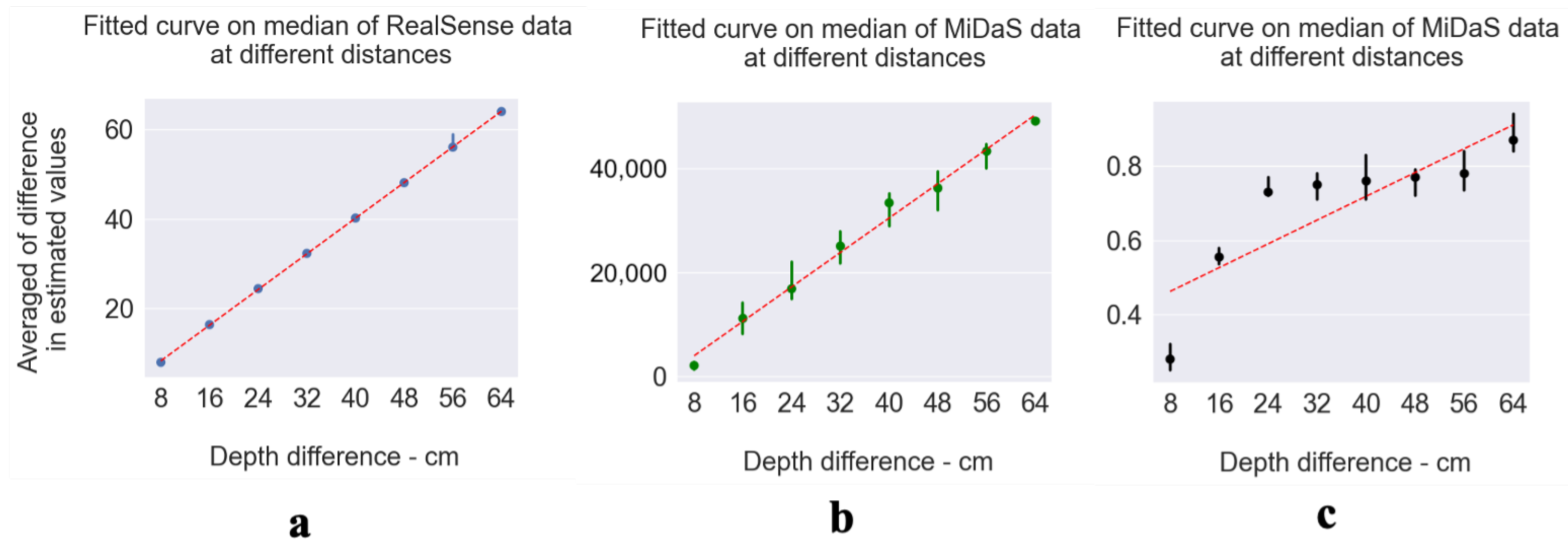
Depth estimation by means of Deep Learning models exploiting an RGB 2D image can be quite noisy and can be affected by light condition. However, we wanted to test if such models can be useful for estimating the depth difference of a pair of objects in the scene, thus allowing us to infer which object is closer to the camera, and whether this depth estimate is consistent and to what extent it is affected by lighting conditions. To get an answer to this question, we calculated the median values of the averaged depth difference estimates under different lighting conditions for each possible combination over different distances (8 cm to 64 cm) for all three objects. By plotting the median values over different distances, we can fit a line to the points and obtain the coefficient of determination (R-squared) of such linear regression from the perfect line with p-values less than 0.0005 for each method. The perfect diagonal line (with a slope of 45 degrees) indicates that the average of the depth differences is stable for closer and further distances (the difference in distances between each median point is 8 cm).

To evaluate the usefulness of the capability of the MiDaS and Alhashim algorithms to estimate depth differences, we calculated the success rate in discriminating depth differences of each pair in the scene ( distinguishing further distances from closer distances), starting from “d + 16”, which corresponds to 34 cm. Thus, we calculated the correct differentiation of depth estimation in the method for each scene where the object is at different distance and under different lighting condition. In a simple way, we measure the performance of each method in differentiating between, for example, 8 cm (closer) and 16 cm (farther) distances. To measure the performance of each method, we calculated how many times the method was successful in estimating the relative depth between three objects, and divided this by all combinations to determine the method’s success percentage. In this way, we indirectly account for each lighting condition in each scene.

3.6.3. Statistical Analysis on Effect of Light in Depth Difference Estimation

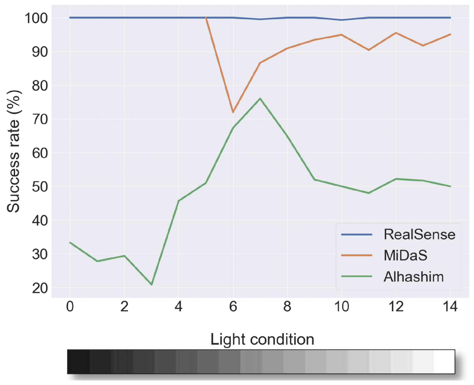
Different lighting conditions affect the quality of image captured by a camera and cause the depth differences between objects to be inconsistent. To get a more accurate idea of the robustness of the two algorithms for estimating depth differences under different lighting conditions, we examine the success rate in discriminating between various differences for three objects at different distances from the camera for each method and each lighting condition.

Accordingly, we calculated how often the algorithms of MiDaS and RealSense are able to detect the correct interactions for the cup and the apple (True Positive—TP), how often the algorithms missed the existing interaction (False Negative—FN), and also how often the algorithms detected a non-existing interaction (False Positive—FP). In addition, it is worth mentioning that we cannot quantify how often the algorithm correctly detected the nonexistent interactions (True Negative—TN), so TN is not applicable in our case.

4. Results

In this section, we will present results of the different depth estimation method and, more importantly, examine the precision of the depth difference in each method. We will also briefly inspect the effects of light on depth estimation. The final part of this section is devoted to the application of depth estimation in hand-object interaction detection.

4.1. Results on Depth Estimation and Its Precision—Experiment A

We examined how measured depths based on RealSense behave under different lighting conditions, and similarly estimated depths in MiDaS and Alhashim. The Figure 9 shows the depth values of all 3 objects corresponding to the different methods.

Figure 9a shows the RealSense data with objects situated like in experiment setup 3 in Figure 4. As we can see, the variance of the values for the right object is surprisingly lower than for the others under different illumination conditions. Moreover, the values are in the range of the real values in centimeters. For the MiDaS method (Figure 9b), we can confirm the progressive trend of depth values with increasing distances. Moreover, the estimated depth values in MiDaS are on the order of 100,000 with unknown scale. In the Alhashim method (Figure 9c), the estimated depth increases with increasing distance and the values are in the range of 0 to 10 without unit. Since we will later compare the results of the depth estimation and the depth difference estimation for each method itself, we do not need to use the same unit for all methods, since this would require additional measurements to find the scale and the shift to obtain absolute measurements in centimeters, and this is not our goal.

In addition, there is a possibility that the figure raises a question regarding the points that can be considered as outliers in the boxplots. However, it is important to consider the fact that these values occur under different illumination conditions and we do not want to ignore the effect of this parameter in our data set. Therefore, we did not remove these points but kept them to consider them in the analysis.

Figure 10 shows the dispersion of the datasets corresponding to the boxplots in the Figure 9. The estimated depth values of the left object at the distances “d + 0” and “d + 8” are more scattered with the MiDaS method than with other methods under different lighting conditions (Figure 10). In addition, the depth of the middle object measured by the RealSense cameras at distances “d + 8” and “d + 16” shows a larger discrepancy in the data than the other methods. It should be noted that the range of the standard deviation is different for the different objects. For example, for the left object there is a high standard deviation (more than 0.8) and for the right object there is a low standard deviation (less than 0.14). But if we look at the Figure 10, we can easily see the big difference between Alhashim and the other methods.

Table 1. Dispersion on measured and estimated values based on different methods.

Method	RealSense	MiDaS	Alhashim
Double of maximum normalized standard deviation corresponding to distance (cm)	5.1	9.8	25.3

reports the quantification of the dispersion of the estimated depth for different methods. As explained in Section 3.6.1, the dispersion is calculated by multiplying the maximum normalized standard deviation by a distance. For example, for the RealSense data, the maximum standard deviation (0.061) is at distance “d + 24”. Thus, the value for RealSense given in Table 1 shows the two standard deviations measured by multiplying 0.061 by “d + 24” twice, which is 2 × (0.061 × 42 cm) = 5.1. In general, the depth estimation is more consistent when the dispersion is smaller. The results show that 95% of the values provided by RealSense have a standard deviation of less than 5.1 cm at different distances and lighting conditions, while this value is 9.8 cm for MiDaS and 25.3 cm for Alhashim (Table 1).

Results on Effect of the Light in Depth Estimation

Poor lighting conditions affect the quality of image captured by a camera and can make object detection and hand-object interaction difficult. To get a more accurate idea of the robustness of the two depth estimation algorithms studied in this work, we computed the average of the depth estimation for each object and for each analysed distance. Figure 11 shows the depth estimate for three lighting samples representing the dark, medium, and light brightness ranges of the scene. The x-axis refers to the different objects and the y-axis refers to the actual distances. For each object, we have studied the effects of light with respect to the different camera-object distances. Figure 11a shows the effects of the minimum depth information that RealSense can provide. We should observe similar colours in the horizontal sections and a slight gradient in the estimated depth in the vertical columns, which is the case for distances greater than 34 centimetres in the RealSense method.

In the MiDaS method in Figure 11b, the values of the estimated depth change as a function of distance and become brighter as the distance increases. However, there are some errors in the middle object that also seem to be present in the RealSense results. This can also be seen in Figure 9b due to the high standard deviation.

On the other hand, for the Alhashim method in Figure 11c, the colour of the cells in each column does not change consistently with the distance in each light condition, indicating poor performance in estimating depth.

4.2. Result on Depth Difference between Two Objects and Its Precision—Experiment A

Figure 12 shows a plot of the median values and the median fitted curve of the averaged depth difference estimates for all different lighting conditions for each possible combination over different distances for all three objects.

As a measure of consistency of the estimated and measured depths, we calculated the coefficient of determination (R-squared) of such linear regression with p-values less than 0.0005 for each method. We obtained that 87% of consistency in the depths measured by RealSense over different lighting conditions and that for MiDaS 59% of consistency. However, only 22% of the depths estimated by Alhashim has consistency over different lighting conditions, as shown in

Table 2. R-squared of median in average of difference at each distance estimated by different Methods.

Method	RealSense	MiDaS	Alhashim
R-Square	0.87	0.59	0.22

.

To assess the practicality of MiDaS & Alhashim’s algorithms in estimating the depth difference, one of the ways is to calculate the correct differentiation of the depth estimation in the method for each setups in Figure 4 within each illumination condition. As shown in

Table 3. Performance of each method in estimating the correct relative depth difference between objects.

Method	RealSense	MiDaS	Alhashim
Range of Distances
Include shortest distance of objects from camera (start at 18 cm to the farthest, which is 98 cm)	86%	93%	58%
Include distances of objects from 34 cm to 98 cm	99%	91%	48%

, we achieved 99% success rate in discriminating depth differences for RealSense, compared to 91% for MiDaS and 48% for Alhashim. These results support the use of the MiDaS method for depth discrimination in our application, as it is able to distinguish which object is closer to the egocentric camera and which object is farthest away, like our off the shelf solution (Intel RealSense Camera).

4.2.1. Result on Effect of Light in Depth Difference Estimation

To investigate the effect of light on depth difference estimation, we examined the success rate in discriminating between distance differences for three objects at different setups (Figure 4) for each method and each illumination condition. We considered distances greater than 34 cm, starting at “d + 16”, since RealSense can only accurately provide a minimum amount of depth information. The Figure 13 shows the results of successfully estimating the depth difference for different illumination conditions. As expected, based on the results in Table 3, RealSense is quite consistent with a high success rate over the selected range of distances (34 cm to 98 cm) for different lighting conditions (99%). Using the MiDaS method for the available data, the smaller value is 72% for light number 6 and 91% for the overall success rate. The reason for the overall lower rate compared to RealSense is due to the two further distances “d + 56” and “d + 64”, where the success rate in estimating the depth corresponding to the distance differences between objects seems to be lower at distances greater than 74 cm than at the closer distances. However, in our application, it is important to monitor hand interaction with objects whose total distance is less than 70 cm, so MiDaS still be a compatible option for our application.

All in all, based on the above analysis and taking into account the disadvantages of 3D (depth) cameras mentioned at the beginning, as well as the advantages of 2D cameras (RGB cameras), we decided to use a 2D camera in our application and to use MiDaS for depth estimation in hand-object interaction detection.

4.3. Performance in Hand-Object Interaction Detection—Experiment B

To evaluate MiDaS in the hand-object interaction detection application, we compared the number of detected interactions based on the RealSense depth data and estimated depth by MiDaS (

Table 4. Summary of Confusion matrices for two selected methods.

Method	RealSense	MiDaS
TP	81	77
FP	28	34
FN	4	9
Total No. of Interactions	86	86

).

We mentioned that we recorded 100 interactions, but as you can see in the Table 4, there are 86 interactions because we focused only on the interactions where the algorithm could detect both the hand and the object in the same frame.

For hand-object interactions, it is important for a reliable performance that the system does not detect activity that does not exist. Therefore, it is especially important that there are fewer FP cases. To determine the reason for the 34 cases in MiDaS, we reviewed the images that were incorrectly detected as interactions. As you can see in the Figure 14, there is an interaction between hand and apple, but no interaction between hand and cup. Since we have two criteria to report the interaction, we can see the difference in depth between the hand and the cup. Also, the difference between the pixels is very small, so the system incorrectly detected this as an interaction between the hand and the cup. Fortunately, this kind of FP cases can be mitigated by adding a third criterion, such as the speed of the hand and the object. So, in this case, if we compute the velocity of the apple, the hand and the cup, we will see that the system can easily detect the interaction between the hand and the apple and not with the cup in these images, since the velocity of the cup is about zero in the different images.

More importantly, the system is able to detect the difference in depth between different objects and the hand, as confirmed by the results in the table. This is because in order to report the interaction (TP), the system must be consistent in measuring the difference of depth between the object and the hand.

The

Table 5. Performance in RealSense and MiDaS.

Method	RealSense	MiDaS
Precision	0.74	0.69
Recall	0.95	0.90
F1-Score	0.84	0.78
Sensitivity	0.95	0.90

shows different performance metrics. We can see that the performances of MiDaS and RealSense are quite similar.

From the above results, we can see that the MiDaS and RealSense results are quite similar if we consider the RealSense results as a kind of ground truth. Precision indicates the percentage of all positive detections that are truly positive: 74% for RealSense and about 70% for MiDaS. Recall, which indicates the percentage of all positive detections that are correct, is also about 90% for the methods. Moreover, the F1 score for RealSense and MiDaS are quite good and close to each other, namely 90% for MiDaS and 95% for RealSense.

5. Discussion

We must take into account that such 3D (depth) cameras usually need to be calibrated according to different lighting conditions in order to provide precise depth estimation. In our application, there is also a possibility that the lighting conditions are different in daily life. So, we do not have the freedom to calibrate for every kind of lighting situation, which is not feasible and also time consuming. This is another reason for possible use of 2D (RGB) cameras in depth estimation.

Based on the results shown in Figure 10, the depth estimation of Alhashim is not as consistent as the results of RealSense and MiDaS at different distances and lighting conditions. Moreover, Alhashim’s results (Section 4.2.1) show that we have a different low success rate in different lighting conditions, which is still lower than the other methods.

Moreover, regarding the effect of light on depth estimation, we observed in Figure 11a that the colours of the display are not stable horizontally at distances less than 34 centimetres. This is because the Intel RealSense camera can only provide accurate depth measurements up to a certain value. However, we observe a colour gradient that shows consistency in both depth estimation and depth difference estimation. In Figure 11b, we can observe the change in light with distance in both vertical and horizontal directions, but of course not as clearly as with the Intel RealSense data (Figure 11a). The results of the Alhashim method, shown in Figure 11c, show a chaotic estimation and do not follow any pattern. It can be concluded that the Alhashim method is intolerant to light changes.

6. Conclusions

Detecting hand-object interactions from an egocentric perspective by using 2D (RGB) cameras instead of 3D (depth) cameras is a first step toward objectively assessing patients’ performance in performing ADLs. To achieve this goal, we first demonstrated the feasibility of replacing depth cameras with 2D cameras while providing depth information. We used Deep Learning Methods for depth reconstruction from RGB images to make this possible.

In this paper, we presented the results of using Deep Learning models for estimating the depth information from only a single RGB image and compared the results with a 3D (depth) camera. We also examined the results under different lighting conditions. The results have shown that one of the methods, MiDaS is robust under different lighting conditions and the other method, Alhashim is very sensitive to different lighting conditions. In addition, we presented the results of using the depth estimated by MiDaS in a hand-object interaction detection task, which is common in ADLs, especially during drinking and eating. The performance of MiDaS has a slightly lower F1 score than that of the 3D (depth) camera but has the advantage of allowing us to envision monitoring patients with more ergonomic 2D (RGB) cameras. Moreover, such cameras are lighter, less bulky, do not need an external source of energy and the means for storage, and most importantly, they have a wider field of view.

For future research, further studies on different depth estimates are needed to apply and compare with the current model in terms of complexity and time. There are potential studies that have shown promising results, e.g., single-stage refinement CNN [26], embedding semantic segmentation by using a hybrid CNN model [27] for depth estimation. In addition, future research could explore the appropriateness of data augmentation in our case, which is consistent with exploring datasets that are more conducive to the research topic. Furthermore, semantic segmentation may be an important component in future object recognition experiments to increase the accuracy of recognition with respect to position of objects in the scene.

In addition, our next step will be to investigate the performance of our hand-object interaction detection system using known databases that are more related to activities of daily life where hands are visible in the scenes.

It is important to mention that in our application we do not guarantee the absolute value of depth, but for us, it is the consistency of providing the depth difference of close objects in the scene that is important, because it can be enough to identify the disposition of the objects in the scene, which one is closer to the camera or to other objects.

The purpose of our hand-object interaction application is to be able to create a log of patients’ interactions and help in the objective assessment of the patient during his/her rehabilitation. Soon, we should be able to extend the use of this technology to the monitoring of patients at home allowing their assessment without the need for hospitalization.