Article

Semantic Segmentation of 12-Lead ECG Using 1D Residual U-Net with Squeeze-Excitation Blocks

Department of Biosensors and Processing of Biomedical Signals, Faculty of Biomedical Engineering, Silesian University of Technology, Roosevelta 40, 41-800 Zabrze, Poland
*
Author to whom correspondence should be addressed.
Appl. Sci. 2022, 12(7), 3332; https://doi.org/10.3390/app12073332
Submission received: 14 February 2022 / Revised: 15 March 2022 / Accepted: 23 March 2022 / Published: 25 March 2022
(This article belongs to the Special Issue New Trends in Machine Learning for Biomedical Data Analysis)

Abstract

:
Analyzing biomedical data is a complex task that requires specialized knowledge. The development of knowledge and technology in the field of deep machine learning creates an opportunity to try and transfer human knowledge to the computer. In turn, this fact influences the development of systems for the automatic evaluation of the patient’s health based on data acquired from sensors. Electrocardiography (ECG) is a technique that enables visualizing the electrical activity of the heart in a noninvasive way, using electrodes placed on the surface of the skin. This signal carries a lot of information about the condition of heart muscle. The aim of this work is to create a system for semantic segmentation of the ECG signal. For this purpose, we used a database from Lobachevsky University available on Physionet, containing 200, 10-second, and 12-lead ECG signals with annotations, and applied one-dimensional U-Net with the addition of squeeze-excitation blocks. The created model achieved a set of parameters indicating high performance (for the test set: accuracy—0.95, AUC—0.99, specificity—0.95, sensitivity—0.99) in extracting characteristic parts of ECG signal such as P and T-waves and QRS complex, regardless of the lead.

1. Introduction

Electrocardiography (ECG) is a golden diagnostic standard for measuring the electrical activity of the heart. This signal has its reflection in the mechanical action of the heart and can inform us about the physiological condition of this organ. The analysis of an electrocardiogram is a complex process that requires specific knowledge. Engineers try to help physicians by creating expert systems. This process requires transfer of the specialist’s knowledge to a computer by feeding it with examples and a set of rules about how to treat specific cases. There are many possibilities of creation of an expert system—one of the most developed is using machine learning-based technologies.
One of the subfields of machine learning methods is deep learning (DL)—containing many hidden layers in the Artificial Neural Network (ANN) structure, which mimics the performance of the human brain [1].
The convolutional neural network, CNN for short, is a specialized type of neural network designed for working with two-dimensional data. It creates rich representations of the input data by sequentially stacking the convolution operations over the image. To reduce the data size, CNNs are often equipped with pooling layers. The filter values are being updated using a backpropagation algorithm. Figure 1 presents a sample of 1D CNN.
These structures can be applied for analyses of physiological signals, such as ECG. The conventional deep convolutional networks are designed to operate exclusively on two-dimensional data. As described in [2], 1D CNNs are more advantageous than their 2D counterparts in dealing with one-dimensional data.
Data annotation is a time-consuming activity, so especially in the era of big data, systems that automatically (but also reliably) label the data are absolutely necessary.

Related Work

The application of deep learning techniques in processing different physiological signals was summarized by Faust et al. They analyzed 53 publications from 1 January 2008 to 31 December 2017, 17 concerning ECGs [3]. Another review of using DL methods for ECG data was performed by Hong et al. in [4]. They evaluated 191 articles published between 1 January 2010 and 29 February 2020. The authors of this work confirm that the application of DL methods in ECG analysis (including signal annotation) is becoming an increasingly frequently discussed topic.
The most frequently discussed issue in relation to the ECG signal is undoubtedly the anomaly detection. Novotna et al. used DL methods for premature ventricular contractions (PVCs) localization. On the CPSC2018 (China Physiological Signal Challenge 2018) database, they achieved the dice coefficient 0.947 for the model with a max pooling layer [5].
Du et al. presented a fine-grained multilabel ECG framework to detect correlated cardiac abnormalities in clinical ECG data using convolutional neural network (CNN) and recurrent neural network (RNN) [6]. The authors of [7] used U-Net with bidirectional LSTM for the automated detection of QRS complexes. They achieved an accuracy of 78.73% and 98.29% on the CPSC2019 (China Physiological Signal Challenge 2019) and mitdb datasets, respectively.
In their work, Weinman and Conrad used transfer learning for improving CNNs classification of heart rhythm and atrial fibrillation (AF) from short ECG signals [8]. The authors explored both unsupervised and supervised pretraining of CNN on the Icentia11K (Icentia11K contains ECG data from 11,000 patients, who wore a monitoring device for up to two weeks resulting in 630,000 h of ECG signal with over 2,700,000,000 beats labeled by the device and then again by a specialist) dataset. They showed that pretraining improves CNN’s performance by over 6% and scored the maximum of F 1 -score 0.926 for beat classification.
Another interesting issue is the analysis of the ECG signal in terms of detecting individual features in physiological biometrics. Zheng et al., in their work, used BP and DNN for ECG-based identification [9]. They created and tested their model on two databases: mitdb (MIT arrhythmia database) and a self-collected one. The database consisted of signals obtained during various emotions. The authors achieved a 94.39% recognition rate on the combined datasets.
An automatic segmentation of a signal, which is nothing more than finding the reference points within it, is crucial in order to perform automatic interpretation of the signal. There are many different algorithms for segmentation of the ECG signal that use many signal processing methods and work on different databases. In their work, Beraza and Romero compared algorithms for ECG segmentation [10]. The authors performed signal segmentation on ECG using nine different algorithms [11,12,13,14,15,16,17,18,19] and PhysioNet’s QT database [20]. They achieved the best results while using probabilistic methods and methods based on wavelet transform.
In our study, we propose an alternative approach for the segmentation of a one-dimensional signal segmentation such as ECG. We created a tool for semantic segmentation that used a one-dimensional U-Net containing squeeze-excitation blocks.

2. Materials and Methods
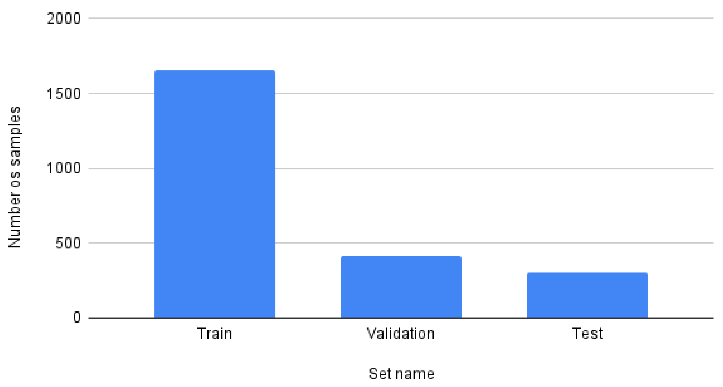
2.1. Dataset

In this study, we used the dataset provided by Lobachevsky University [21], available on the Physionet website. The dataset consists of 200, 10-second, and 12-lead ECG signals, representing different morphologies. Each of the signals comes with an annotation describing the starting, stopping, and peak points of the P and T waves and QRS complexes. The data are compatible with the popular wfdb toolbox. For a more detailed description, please refer to [21].

Data Preparation

In the provided dataset, some of the annotations were incorrect, containing an annotation without the peak point or with it being mislabeled. These samples were removed from the data along with its paired signals. In total, there were 2377 signals with a length of 5000 samples. As mentioned, the annotation came in the form of point collection. To create suitable masks for our model, we transformed the points collection into masks matching the shape of the input signal. For the specific fragments corresponding to the annotations, we applied a label in the form of an integer number as follows:
  • “0”—background;
  • “1”—QRS block;
  • “2”—T-wave;
  • “3”— P-wave.
Then, we took the generated sparse masks that are one-hot-encoded, and the final labels have the shape k × 5000 × 4 , where k indicates the number of samples. The input signals were normalized using the min–max scaling technique, which is defined as:
x = x m i n ( x ) m a x ( x ) m i n ( x ) .
Then, the dataset was split into training, validation, and testing sets as follows: first, we divided the data into a training and testing set with 80% and 20%; then, we extracted 20% of the training set into the validation set. The distribution of the dataset is presented in the Figure 2.
The distributions between categories across the dataset are as follows:
  • Background—7,309,154 points,
  • QRS complex—894,721 points;
  • P-wave—1,516,929 points;
  • T-wave—814,196 points.

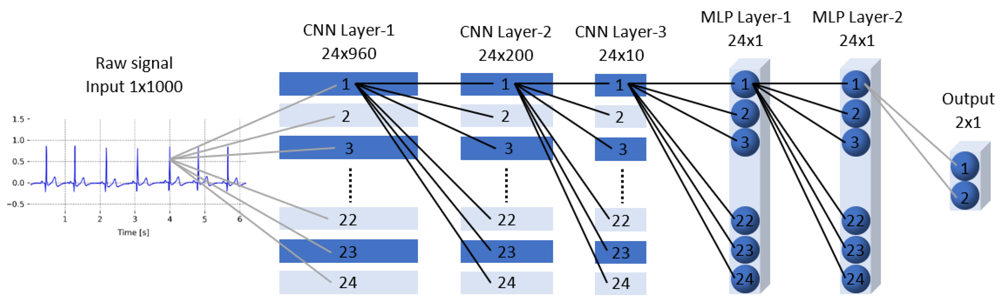
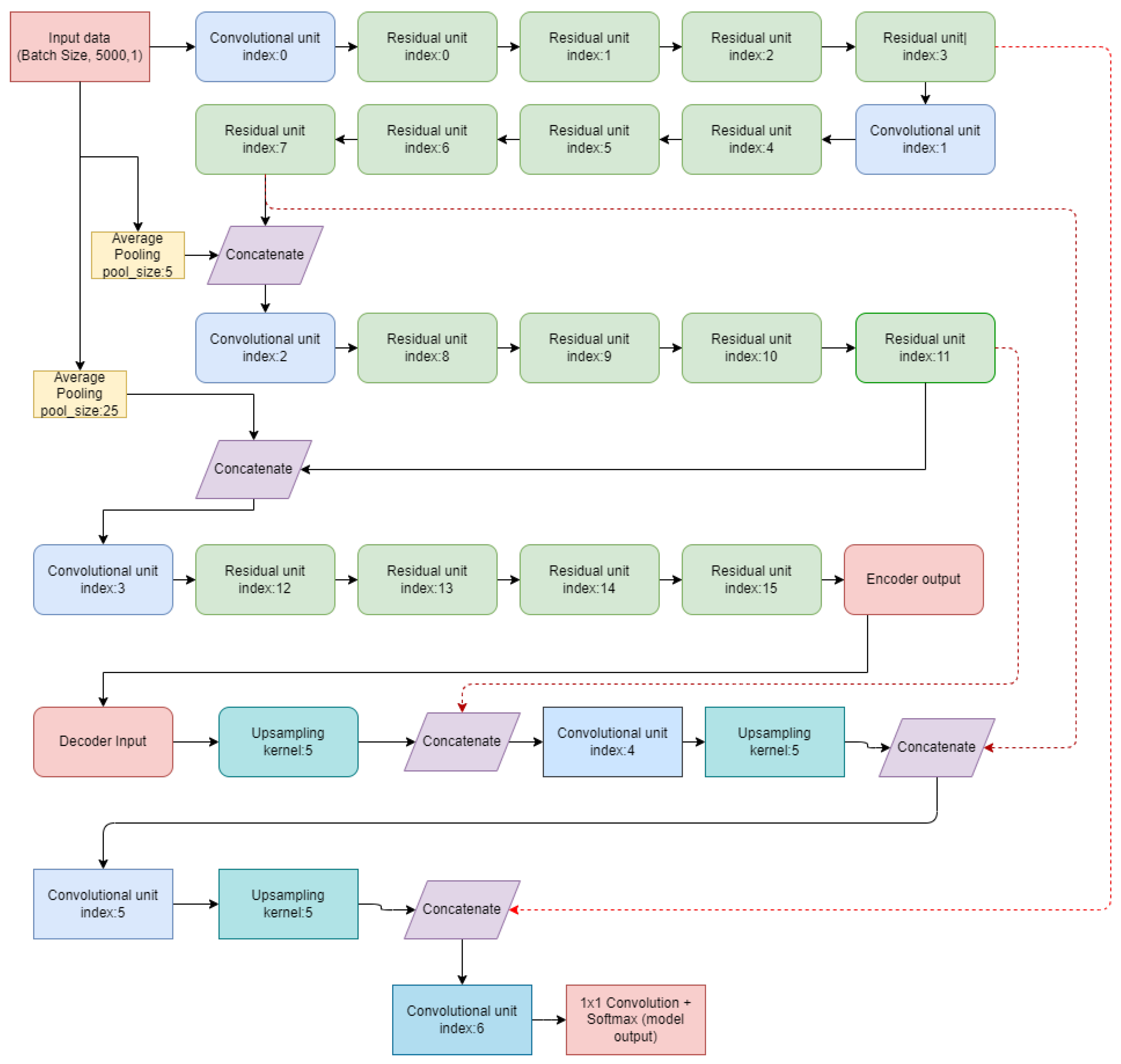
2.2. Model Architecture

For our study, we chose the U-Net architecture design proposed by Ronnenberger et al. [22] and adapted it for the task of 1D semantic segmentation. Inspired by the paper [23], we have decided to incorporate residual and squeeze-excitation blocks into our model. A diagram of the model architecture is presented in Figure 3. A full diagram of the model is available as supplementary material (File S1).

2.2.1. Encoder

The encoder part of our network is a modified ResNet [24] convolutional neural network. It was designed with four sequentially connected blocks. The single block was made of 3 functional units:
  • Convolutional unit—this unit consists of a one-dimensional convolutional layer followed by batch normalization [25];
  • Squeeze-exciting unit—is a cell designed to improve the representational power of a network by enabling it to perform channel-wise feature calibration. The inputs to this block are the feature maps generated by the convolutional unit. Each of the channels is being “squeezed” into a single numeric value using global average pooling. This value will be passed through two feed-forward layers activated by the ReLU and sigmoid functions to add nonlinearity and give each channel a smooth gating function. Then, the output of the sigmoid function is weighted by the input feature maps to get the excitation [26];
  • Residual unit—this unit stacks two convolutional units, and on top of them, the squeeze-exciting unit is being stacked. The output is being added to the input feature maps.
The encoder consists of four of these blocks as a single convolutional unit followed by four consecutive residual blocks. The outputs of the second and third block are being concatenated with the averaged pooled input data.

2.2.2. Decoder

The decoder part consists of up-sampling layers followed by concatenation with encoder feature maps and convolutional units. In total, there were 34,305,156 parameters from which 34,816 were not trainable.

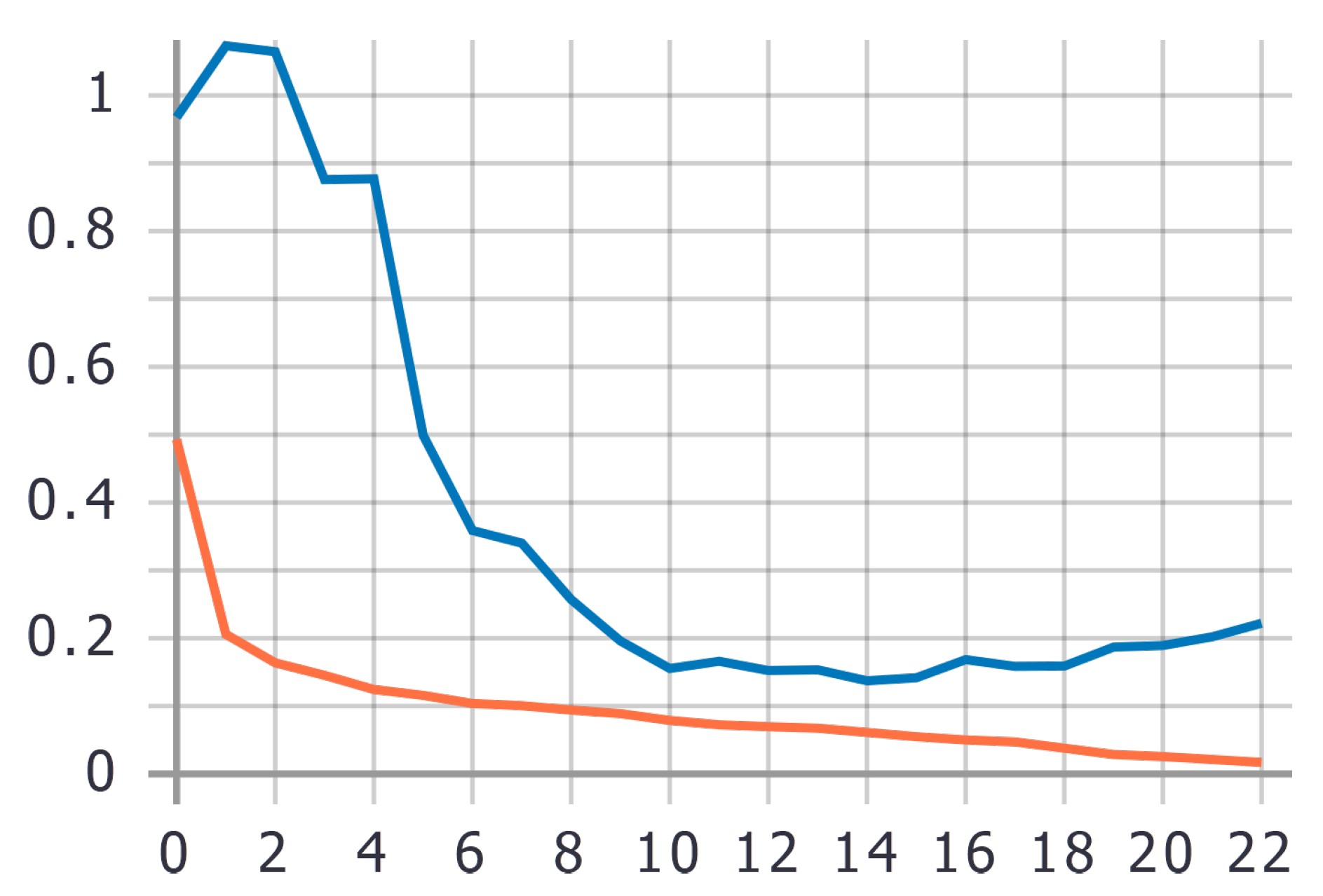
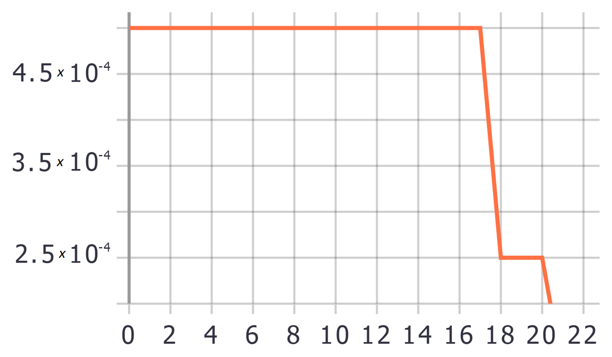
2.3. Training Process

The training procedure was conducted using the Adam optimization algorithm [27] and categorical cross-entropy as the loss function. We have examined two versions of our model—one with and one without squeeze-exciting blocks. Both models were trained with the following parameters:
  • 32 mini-batch size;
  • starting learning rate of 0.0005.
The hyperparametrs were tuned empirically. For this procedure, we have defined a set of callbacks to prevent overfitting and optimize learning:
  • Model checkpoint—saving the model that achieves the best validation loss score;
  • Reduce learning rate—dynamic learning rate set to decrease by half each 3 epochs when the validation loss is not improving;
  • Early stopping—stopping the training procedure when the model overfits the data (after 3 epochs).
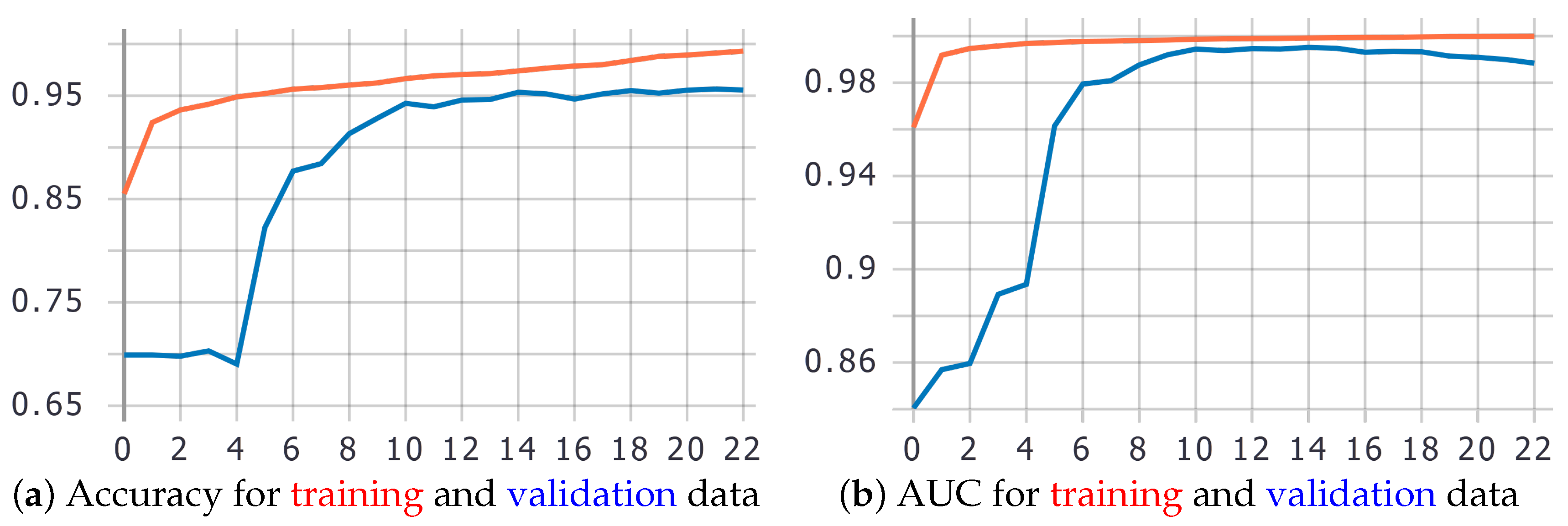
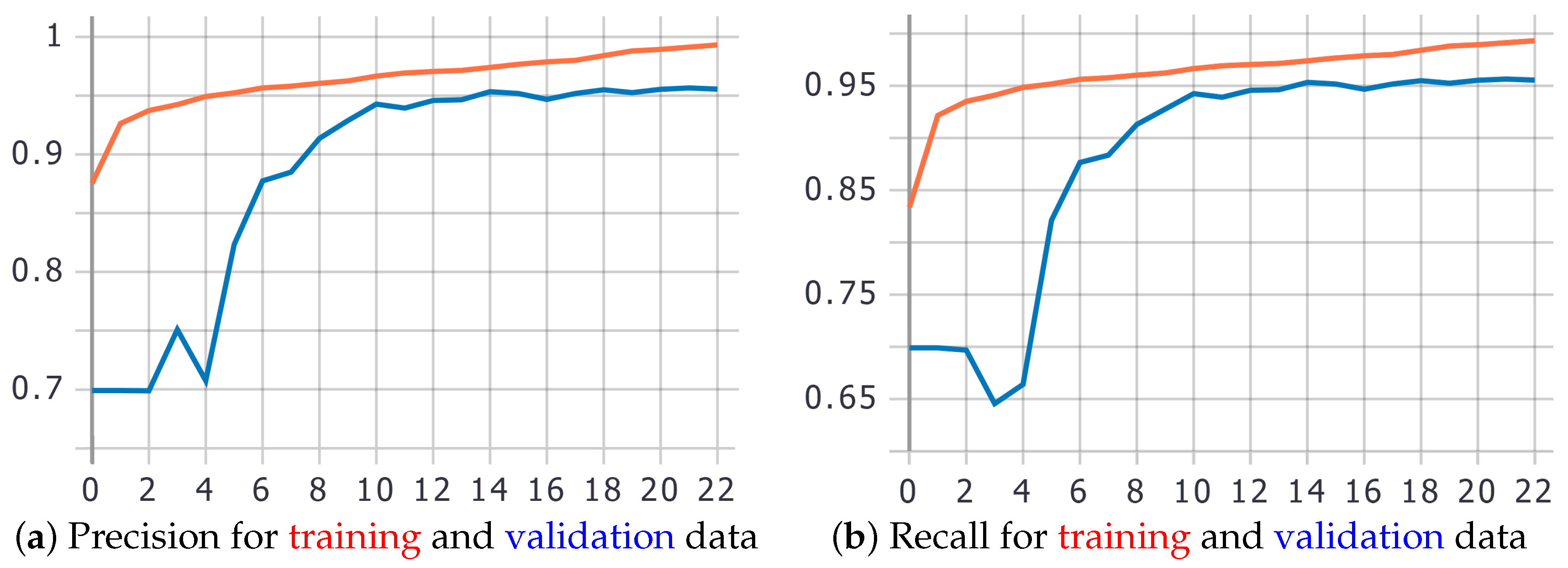
The model was set to be trained for 100 epochs, but after 20 epochs, the early stopping callback stopped the learning process due to overfitting. The model with the best validation loss was saved.
The described model was trained on an NVIDIA RTX 2080Ti graphics card with 12 GB of video RAM. The model was designed with the help of Tensorflow and Keras deep learning libraries.

3. Results

This section provides numerical and visual results of the training, validation, and testing of the proposed models. We compared the models with and without the addition of squeeze-exciting blocks.

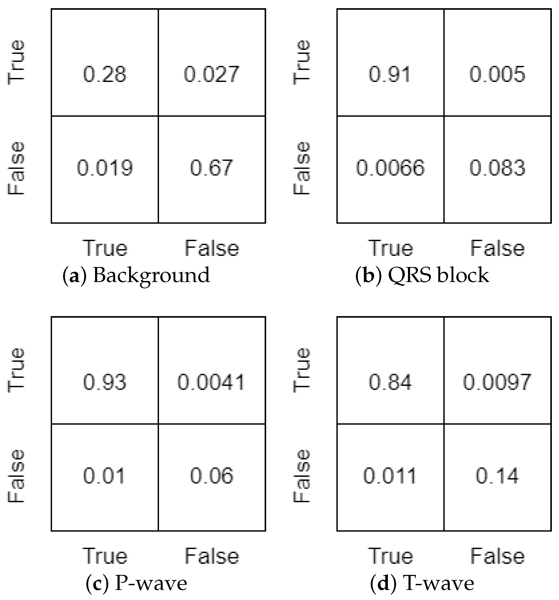
3.1. Numerical Results

To examine the overall model performance, we calculated standard metrics, such as precision, recall, and area under the ROC curve. The numerical results are presented for two versions of the model—with and without squeeze-exciting blocks. The comparison between these two models is shown in Table 1.
When evaluating on the test set, the Jaccard index [28] and the F1-score were also defined to properly test the trained models (see Table 2). The Jaccard index J ( A , B ) and F1-score F 1 ( A , B ) are defined as follows:
J ( A , B ) = | A B | | A B | ,
F 1 ( A , B ) = 2 · | A B | | A | + | B | ,
where A B is the intersection of sets A and B, and A B is the union of sets A and B.
As we are dealing with a multi-class segmentation problem, the aforementioned indicators were calculated in three different variants: micro, macro, and weighted. With the ‘micro’ variant, we calculate metrics globally, i.e., by counting the total true positives, true negatives, false negatives, and false positives. For the ‘macro’ variant, we calculate metrics for each label, and then, we calculate their unweighted mean. This does not take label imbalance into account. In case of the ‘weighted’ variant, we calculate metrics for each label and find their average, which is weighted by the number of true instances for each label. This alters ‘macro’ to account for label imbalance.
Based on the results presented in Table 2, we can see that the squeeze-excitation blocks enhance the overall performance of the model. They also provide a better generalization of the problem, which can be seen by analyzing the loss function across different sets.
The learning curves are presented for the model that contains squeeze-excitation blocks since it yields better results (see Figure 4, Figure 5, Figure 6, Figure 7 and Figure 8).
Accuracy is a percent of correct predictions. It describes the performance of the model among classes. Accuracy is given by the following formula [29]:
A c c u r a c y = T P + T N T P + F P + T N + F N ,
where TP—true positive value, TN—true negative value, FP—false positive value, FN—false negative value (applies to Formulas (4)–(8)).
AUC, Area Under the ROC Curve, provides information on how well the model distinguishes between the classes. The desired value is an AUC as close as possible to 1.
Specificity is a metric that describes the model’s ability to correctly predict the true negative value. Specificity is given by the following formula [29]:
S p e c i f i c i t y = T N T N + F P .
Sensitivity is a metric that describes the model’s ability to correctly predict the true positive value. Sensitivity is given by the following formula [29]:
S e n s i t i v i t y = T P T P + F N .
In this case, to determine the sensitivity, we first compute specificity at 200 different thresholds ( t h r e s h o l d n = t h r e s h o l d n 1 2 ; n = 1 , 2 , 3 , , 200 ; t h r e s h o l d 0 = 1 ). Then, the sensitivity is computed at the chosen threshold [30].
When the model achieves high specificity and sensitivity values after the learning cycle, that means that the results are reliable.
Precision is a ratio between the number of true positive samples and all samples classified as positive (i.e., the sum of true and false positive samples). This metric shows the model’s ability to correctly classify positive samples. Precision is given by the following formula [29]:
P r e c i s i o n = T P T P + F P .
Recall is a metric that defines how well the model detects the positive samples. It is calculated as a ratio between true positive samples and all positive samples (that is, the sum of true positive and false negative samples).
R e c a l l = T P T P + F N .
Loss, in other words, penalty for a bad prediction, is a value that indicates how bad the model prediction was on a single sample. In simple terms—the lower the loss, the better the model.
We have calculated the percentage of correctly classified samples for each class and presented it in the form of confusion matrices. Figure 9 shows confusion matrices for each class for the test dataset.
The percentage of correctly classified samples can be calculated as the sum of the values on the main diagonal. For the test dataset, the model scored the following values for each class:
  • background—95%;
  • QRS block—99.3%;
  • P wave—99%;
  • T wave—98%.

3.2. Visual Results

To compare predictions of the created model with the original annotations, we chose three examples of signals from the test dataset. As the model containing the squeeze-exciting blocks achieved better results, only its predictions were visualized.
Figure 10 show signals with masks presented as follows:
  • black—background (0);
  • red—QRS block (1);
  • blue—T wave (2);
  • cyan—P wave (3).
In the figure, we can see that the model correctly segmented all the aforementioned ECG fragments regardless of the signal lead.

4. Discussion

In this work, we presented a solution for extracting P and T-waves and QRS complexes from 12-lead ECG signals using methods that are mostly used in the image processing domain. The created model achieves a high set of performance parameters (accuracy, AUC, specificity, and sensitivity) independently on all signal leads. Thanks to this, our solution can be used in any type of electrode configuration as a basis for heart rhythm and heart rate variability (HRV) classification as well as many other parameters resulting from specific fragments of ECG. Using our method, we obtained results comparable or better than those presented in the literature [3,4,5,6,7,8,9,10,11,12,13,14,15,16,17,18,19].
According to the World Health Organization (WHO), the top cause of death worldwide in 2019 was ischemic heart disease [31], also showing the biggest increase in deaths since 2000. This disease has its representation in ECG as ST-segment elevation or depression. Taking into account the growing popularity of wearable devices (e.g., a smart watch or a smart band equipped with a simple ECG recorder), we have a chance for earlier detection of cardiovascular disorders by applying real-time segmentation methods and ECG analysis on an everyday basis for high-risk patients.
The deep learning approach seems to be an effective solution to the problem of medical signal segmentation. Considering the ability of neural networks to capture highly nonlinear patterns and their efficient feature extraction process, it can be used to help diagnose patients based on the signals captured from their body. These solutions are yielding state-of-the-art results and can be adopted as preliminary diagnosis systems.
For solving the problem of semantic segmentation of ECG, we have chosen to use U-Net like architecture. This solution has a few advantages. First, convolutions are less computationally expensive than for example the transformer model, which adopts point-wise dependencies discovery, whose complexity increases quadratically with the length of the time series, which given a time series of a 5000-samples length can easily become intractable. In turn, the lower computation cost can be advantageous when trying to incorporate neural network models onto microprocessors to work directly on hardware. Given the nature of the problem—recognizing sequentially repeating signals—using convolution seems to be a suitable solution since it is sensitive to a local neighborhood of values.
A significant challenge in creating a system for ECG segmentation is finding an appropriate database for training the model or classifier. For this purpose, signal generators can be used, such as the one proposed by Stabenau et al. [32]. Artificial signals can be used to pretrain models that then are tuned to a real data.
In the future, we plan to replace the up-sampling layers of the decoder with one-dimensional transposed convolution layers that have learnable parameters. Based on the success of the transformer architecture [33] in natural language processing, we also consider replacing the convolution-based feature extractor with the mentioned architecture. In the future work, besides architectural changes, we also plan to extend our dataset with new categories that represent both healthy P and T-waves, ORS-complexes, and pathological. Another direction worth exploring in the future research is the use of a semantic segmentation approach to detect more complex, and non-sequential events in biomedical signals comparing a wider range of architectures, from 1D convolutional networks, Performer [34], and Linformer [35] and new architectures that seem to be a bridge between the two [36].

Supplementary Materials

The following supporting information can be downloaded at: https://www.mdpi.com/article/10.3390/app12073332/s1. File S1: Full diagram of the proposed model.

Author Contributions

Conceptualization, K.D. and P.K.; methodology, K.D. and N.P.; software, K.D.; validation, K.D. and P.K.; formal analysis, K.D. and N.P.; investigation, K.D. and E.T.; resources, K.D.; data curation, K.D.; writing—original draft preparation, K.D. and N.P.; writing—review and editing, K.D., N.P., P.K. and E.T.; visualization, K.D. and N.P.; supervision, P.K. and E.T.; project administration, N.P.; funding acquisition, K.D. and E.T. All authors have read and agreed to the published version of the manuscript.

Funding

This study was carried out under the project “InterPOWER—Silesian University of Technology as a modern European technical university”, co-financed by the European Union under Measure 3.5 Comprehensive programs of universities III Priority Axis Higher education for the economy and development of the Operational Program Knowledge Education Development 2014–2020.

Conflicts of Interest

The authors declare no conflict of interest.

Abbreviations

The following abbreviations are used in this manuscript:
AFAtrial Fibrillation
ANNArtificial Neural Network
AUCArea Under the Curve
CNNConvolutional Neural Network
DLDeep Learning
ECGElectrocardiography
HRVHear Rate Variability
PVCPremature Ventricular Contractions
ReLURectified Linear Unit
RNNRecurrent Neural Network
WHOWorld Health Organization

References

  1. Goodfellow, I.; Bengio, Y.; Courville, A. Deep Learning; Adaptive Computation and Machine Learning; The MIT Press: Cambridge, MA, USA, 2016. [Google Scholar]
  2. Kiranyaz, S.; Avci, O.; Abdeljaber, O.; Ince, T.; Gabbouj, M.; Inman, D.J. 1D convolutional neural networks and applications: A survey. Mech. Syst. Signal Process. 2021, 151, 107398. [Google Scholar] [CrossRef]
  3. Faust, O.; Hagiwara, Y.; Hong, T.J.; Lih, O.S.; Acharya, U.R. Deep learning for healthcare applications based on physiological signals: A review. Comput. Methods Programs Biomed. 2018, 161, 1–13. [Google Scholar] [CrossRef] [PubMed]
  4. Hong, S.; Zhou, Y.; Shang, J.; Xiao, C.; Sun, J. Opportunities and Challenges of Deep Learning Methods for Electrocardiogram Data: A Systematic Review. arXiv 2020, arXiv:2001.01550. [Google Scholar] [CrossRef] [PubMed]
  5. Novotna, P.; Vicar, T.; Hejc, J.; Ronzhina, M.; Kolarova, J. Deep-Learning Premature Contraction Localization in 12-lead ECG From Whole Signal Annotations. In Proceedings of the Computing in Cardiology, Rimini, Italy, 13–16 September 2020. [Google Scholar] [CrossRef]
  6. Du, N.; Cao, Q.; Yu, L.; Liu, N.; Zhong, E.; Liu, Z.; Shen, Y.; Chen, K. FM-ECG: A fine-grained multi-label framework for ECG image classification. Inf. Sci. 2021, 549, 164–177. [Google Scholar] [CrossRef]
  7. He, R.; Liu, Y.; Wang, K.; Zhao, N.; Yuan, Y.; Li, Q.; Zhang, H. Automatic Detection of QRS Complexes Using Dual Channels Based on U-Net and Bidirectional Long Short-Term Memory. IEEE J. Biomed. Health Inform. 2021, 25, 1052–1061. [Google Scholar] [CrossRef]
  8. Weimann, K.; Conrad, T.O.F. Transfer learning for ECG classification. Sci. Rep. 2021, 11, 5251. [Google Scholar] [CrossRef]
  9. Zheng, G.; Ji, S.; Dai, M.; Sun, Y. ECG Based Identification by Deep Learning. In Biometric Recognition; Zhou, J., Wang, Y., Sun, Z., Xu, Y., Shen, L., Feng, J., Shan, S., Qiao, Y., Guo, Z., Yu, S., Eds.; Springer International Publishing: Cham, Switzerland, 2017; Volume 10568, pp. 503–510. [Google Scholar] [CrossRef]
  10. Beraza, I.; Romero, I. Comparative study of algorithms for ECG segmentation. Biomed. Signal Process. Control 2017, 34, 166–173. [Google Scholar] [CrossRef]
  11. Laguna, P.; Jané, R.; Caminal, P. Automatic Detection of Wave Boundaries in Multilead ECG Signals: Validation with the CSE Database. Comput. Biomed. Res. 1994, 27, 45–60. [Google Scholar] [CrossRef]
  12. Martinez, J.; Almeida, R.; Olmos, S.; Rocha, A.; Laguna, P. A Wavelet-Based ECG Delineator: Evaluation on Standard Databases. IEEE Trans. Biomed. Eng. 2004, 51, 570–581. [Google Scholar] [CrossRef]
  13. Singh, Y.N.; Gupta, P. ECG to Individual Identification. In Proceedings of the 2008 IEEE Second International Conference on Biometrics: Theory, Applications and Systems, Washington, DC, USA, 29 September–1 October 2008; pp. 1–8. [Google Scholar] [CrossRef]
  14. Di Marco, L.Y.; Chiari, L. A wavelet-based ECG delineation algorithm for 32-bit integer online processing. Biomed. Eng. Online 2011, 10, 23. [Google Scholar] [CrossRef] [Green Version]
  15. Sun, Y.; Chan, K.L.; Krishnan, S.M. Characteristic wave detection in ECG signal using morphological transform. BMC Cardiovasc. Disord. 2005, 5, 28. [Google Scholar] [CrossRef] [PubMed] [Green Version]
  16. Martínez, A.; Alcaraz, R.; Rieta, J.J. Application of the phasor transform for automatic delineation of single-lead ECG fiducial points. Physiol. Meas. 2010, 31, 1467–1485. [Google Scholar] [CrossRef] [PubMed]
  17. Vázquez-Seisdedos, C.R.; Neto, J.E.; Marañón Reyes, E.J.; Klautau, A.; Limão de Oliveira, R.C. New approach for T-wave end detection on electrocardiogram: Performance in noisy conditions. BioMed. Eng. Online 2011, 10, 77. [Google Scholar] [CrossRef] [PubMed] [Green Version]
  18. Vitek, M.; Hrubes, J.; Kozumplik, J. A Wavelet-Based ECG Delineation with Improved P Wave Offset Detection Accuracy. Anal. Biomed. Signals Images 2010, 20, 160–165. [Google Scholar]
  19. Hughes, N.P.; Tarassenko, L.; Roberts, S.J. Markov Models for Automated ECG Interval Analysis. In Proceedings of the NIPS 2003, Vancouver, BC, Canada, 8–13 December 2003. [Google Scholar]
  20. Laguna, P.; Mark, R.; Goldberg, A.; Moody, G. A database for evaluation of algorithms for measurement of QT and other waveform intervals in the ECG. In Proceedings of the Computers in Cardiology 1997, Lund, Sweden, 7–10 September 1997; IEEE: Lund, Sweden, 1997; pp. 673–676. [Google Scholar] [CrossRef]
  21. Kalyakulina, A.; Yusipov, I.; Moskalenko, V.; Nikolskiy, A.; Kosonogov, K.; Zolotykh, N.; Ivanchenko, M. Lobachevsky University Electrocardiography Database. Type: Dataset. Available online: https://physionet.org/content/ludb/1.0.0/ (accessed on 10 July 2021).
  22. Ronneberger, O.; Fischer, P.; Brox, T. U-Net: Convolutional Networks for Biomedical Image Segmentation. arXiv 2015, arXiv:1505.04597. [Google Scholar]
  23. Yan, W.; Hua, Y. Deep Residual SENet for Foliage Recognition. In Transactions on Edutainment XVI; Pan, Z., Cheok, A.D., Müller, W., Zhang, M., Eds.; Springer: Berlin/Heidelberg, Germany, 2020; Volume 11782, pp. 92–104. [Google Scholar] [CrossRef]
  24. He, K.; Zhang, X.; Ren, S.; Sun, J. Deep Residual Learning for Image Recognition. arXiv 2015, arXiv:1512.03385. [Google Scholar]
  25. Ioffe, S.; Szegedy, C. Batch Normalization: Accelerating Deep Network Training by Reducing Internal Covariate Shift. arXiv 2015, arXiv:1502.03167. [Google Scholar]
  26. Hu, J.; Shen, L.; Albanie, S.; Sun, G.; Wu, E. Squeeze-and-Excitation Networks. arXiv 2019, arXiv:1709.01507. [Google Scholar]
  27. Kingma, D.P.; Ba, J. Adam: A Method for Stochastic Optimization. arXiv 2017, arXiv:1412.6980. [Google Scholar]
  28. Jaccard, P. The distribution of the flora in the alpine zone. 1. New Phytol. 1912, 11, 37–50. [Google Scholar] [CrossRef]
  29. Tharwat, A. Classification assessment methods. Appl. Comput. Inform. 2021, 17, 168–192. [Google Scholar] [CrossRef]
  30. Keras—Sensitivity at Specificity|TensorFlow Core v2.8.0. Available online: https://www.tensorflow.org/api_docs/python/tf/keras/metrics/SensitivityAtSpecificity (accessed on 14 March 2022).
  31. The Top 10 Causes of Death. Available online: https://www.who.int/news-room/fact-sheets/detail/the-top-10-causes-of-death (accessed on 25 June 2021).
  32. Stabenau, H.F.; Bridge, C.P.; Waks, J.W. ECGAug: A novel method of generating augmented annotated electrocardiogram QRST complexes and rhythm strips. Comput. Biol. Med. 2021, 134, 104408. [Google Scholar] [CrossRef] [PubMed]
  33. Vaswani, A.; Shazeer, N.; Parmar, N.; Uszkoreit, J.; Jones, L.; Gomez, A.N.; Kaiser, L.; Polosukhin, I. Attention Is All You Need. arXiv 2017, arXiv:1706.03762. [Google Scholar]
  34. Choromanski, K.; Likhosherstov, V.; Dohan, D.; Song, X.; Gane, A.; Sarlos, T.; Hawkins, P.; Davis, J.; Mohiuddin, A.; Kaiser, L.; et al. Rethinking Attention with Performers. arXiv 2020, arXiv:2009.14794. [Google Scholar]
  35. Wang, S.; Li, B.Z.; Khabsa, M.; Fang, H.; Ma, H. Linformer: Self-Attention with Linear Complexity. arXiv 2020, arXiv:2006.04768. [Google Scholar]
  36. Li, D.; Hu, J.; Wang, C.; Li, X.; She, Q.; Zhu, L.; Zhang, T.; Chen, Q. Involution: Inverting the Inherence of Convolution for Visual Recognition. arXiv 2021, arXiv:2103.06255. [Google Scholar]
Figure 1. A sample 1D CNN with three-convolutional and two-linear layers [2].
Applsci 12 03332 g001
Figure 2. Data distribution.
Applsci 12 03332 g002
Figure 3. Diagram of the model.
Applsci 12 03332 g003
Figure 4. Learning curves—accuracy and AUC among the epochs.
Applsci 12 03332 g004
Figure 5. Learning curves—specificity and sensitivity among the epochs.
Applsci 12 03332 g005
Figure 6. Learning curves—precision and recall among the epochs.
Applsci 12 03332 g006
Figure 7. Loss on training and validation data among the epochs.
Applsci 12 03332 g007
Figure 8. Learning rate among the epochs.
Applsci 12 03332 g008
Figure 9. Confusion matrices for each class for the test dataset.
Applsci 12 03332 g009
Figure 10. The result of the segmentation using the model on all twelve leads of the ECG signal.
Applsci 12 03332 g010
Table 1. Comparison between metrics achieved without and with squeeze-exciting blocks for the train, validation, and test datasets.
Without Squeeze-ExcitingWith Squeeze-Exciting
DatasetTrainValidationTestTrainValidationTest
Accuracy0.970.920.920.970.950.95
AUC0.990.980.980.990.990.99
Specificity1.00.990.970.990.990.95
Sensitivity1.00.990.990.990.990.99
Recall0.970.920.920.980.950.95
Precision0.970.920.920.970.950.95
Loss0.060.250.390.060.140.14
Table 2. Comparison of the Jaccard index and F1-score achieved without and with squeeze-exciting blocks for the test dataset.
Jaccard IndexF1-Score
MacroMicroWeightedMacroMicroWeighted
Without squeeze-exciting0.80.860.860.870.920.92
With squeeze-exciting0.870.910.910.930.960.96
Publisher’s Note: MDPI stays neutral with regard to jurisdictional claims in published maps and institutional affiliations.

