Abstract
Anatomical realistic voxel models of human beings are commonly used in numerical dosimetry to evaluate the human exposure to low-frequency electromagnetic fields. The downside of these models is that they do not correctly reproduce the boundaries of curved surfaces. The stair-casing approximation errors introduce computational artifacts in the evaluation of the induced electric field and the use of post-processing filtering methods is essential to mitigate these errors. With a suitable exposure scenario, this paper shows that tetrahedral meshes make it possible to remove stair-casing errors. However, using tetrahedral meshes is not a sufficient condition to completely remove artifacts, because the quality of the tetrahedral mesh plays an important role. The analyses carried out show that in real exposure scenarios, other sources of artifacts cause peak values of the induced electric field even with regular meshes. In these cases, the adoption of filtering techniques cannot be avoided.
1. Introduction
Low-frequency (LF) numerical dosimetry is an active research field due to some unresolved issues that still require to be addressed [1,2]. The evaluation of human exposure to the electromagnetic field requires an evaluation of the maximum value of the induced electric field in the human body. The use of the raw solution is, however, subject to numerical artifacts stemming from different sources [3]. One common source of numerical artifacts is the so called stair-casing effect, due to the reconstruction of the body tissues using cubic elements (voxels) coming directly from DICOM (Digital Imaging and Communications in Medicine) images [4]. Voxel-based meshes are intrinsically unable to match curved boundaries, as shown in Figure 1.
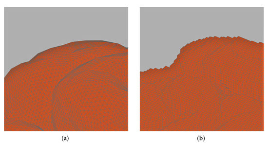
Figure 1.
No stair-casing effect on curved boundaries thanks to tetrahedral discretization (a). Stair-casing effect on curved boundaries due to the use of a voxel-based mesh (b).
Numerical artifacts cause an overestimation of the exposure and must therefore be filtered out with specific methods proposed in standards, guidelines and the literature [5,6,7]. One possible solution to remove the stair-casing errors is the use of tetrahedral meshes. Over the last decades, thanks to the use of geometric modelling software, the organs and tissues of human models derived from DICOM images have been reconstructed using three-dimensional mathematical primitives (e.g., NURBS), giving the possibility to generate tetrahedral meshes that better reproduce the boundaries of curved surfaces. Human models discretized with tetrahedral meshes started to be used both in low-frequency and high-frequency numerical dosimetry (see, for example, [8] where a procedure to optimize the specific absorption rate deposed in a patient during oncological hyperthermia treatment is presented). In [9,10], an anatomical model of the human body composed of tetrahedral elements and obtained from CT scans was used. The aim was to validate new methodologies based on A- finite elements formulation to compute the induced currents into the human body due to LF magnetic fields generated, respectively, by realistic devices and completely unknown power sources. In [11], two dual finite elements formulations to perform numerical dosimetry are presented. Two human models discretized with tetrahedral elements are used in the analysis of numerical errors related to the proposed methodology: the ZOL phantom built using the software AMIRA starting from the segmented data of the Visible Human Project® (VHP), and the Ella phantom based on the Virtual Family, whose tetrahedral mesh was generated from the voxel model by means of the free Matlab toolbox iso2mesh [12]. It is interesting to note that in these papers the authors’ attention is focused on the validation of the new proposed formulations rather than the effects of tetrahedral meshes on numerical artifacts. The question of the influence of the quality of the mesh on computational results is explicitly addressed in [13], where it is proposed to use a local a posteriori residual estimator to evaluate the error.
A comparison between tetrahedral and voxel-based meshes is the main objective of this paper. Regarding this aspect, some results are already available in the literature. In [14], the authors validated their method on the tetrahedral human model ZOL and the numerical results are compared with some existing data evaluated on voxelized human models. The comparison showed some inconsistencies between the data obtained with the tetrahedral models and with the voxel-based ones. The authors underlined the difficulties in comparing different models and methods due to the fact that discretization and post-processing techniques play an important role in the process. However, they did not perform a detailed analysis on the nature of the numerical artifacts present in tetrahedral and voxel-based meshes and no conclusions can be drawn from their analysis. In [15], the authors compared the use of voxel and tetrahedral meshes with the idea of eliminating the staircasing effect with tetrahedral meshes. Computations were performed using five 3D head models obtained from magnetic resonance imaging. The solution obtained with the smallest voxels (edge length of ) was taken as reference. Homogeneous and localized exposure were considered and, although tetrahedral meshes improved the representation of the tissue boundaries, numerical artifacts were registered and filtering techniques were still necessary. The authors conclude that low quality elements in the dosimetric domain are the reason for the failure of tetrahedral meshes in removing numerical artifacts.
In this paper, we analyze the problem from another point of view. A specific methodology is used to identify the source of numerical artifacts produced by tetrahedral meshes to provide additional details about their role in low-frequency numerical dosimetry. Simplified and realistic 3D human models are used in numerical simulations. In particular, simulations are performed on: (1) simple 3D models that also have an analytical solution, (2) 3D models that can be studied with a 2D equivalent simulation used as reference solution, (3) anatomical 3D models that make it possible to investigate the results in real exposure conditions. It is shown that in real exposure scenarios, similarly to the conclusions in [15], numerical artifacts still require filtering techniques to be removed. However, taking advantage of specific exposure scenarios where the unique source of numerical artifacts is the stair-casing, it is shown that tetrahedral meshes are able to completely remove the errors related to geometrical modeling of the computational domain. Furthermore, it is shown that numerical artifacts can also occur in tetrahedra with very high quality if they belong to a boundary characterized by high contrast of the conductivity value. Therefore, in this paper we provide further clarifications about the role of tetrahedral meshes in numerical dosimetry with special attention to the artifacts originating from stair-casing approximation of curved boundaries of human models.
2. Numerical Formulation
In low frequency numerical dosimetry, the currents induced in the human body are too weak to modify the source field, hence human exposure can be assessed by means of the well-known scalar potential finite difference (SPFD) technique, where the magnetic field can be considered as the unperturbed source of the problem [16]. This method has been employed extensively in the literature [17,18,19,20,21,22,23]. The finite integration technique (FIT) using the nodal electric scalar potential as unknowns can be considered as a generalization of the SPFD to tetrahedral meshes, and it is used in this paper for both voxel and tetrahedral discretizations. Under this hypothesis, the linear system is
where is the edge-to-node incidence matrix, is the conductance matrix, is the vector of nodal electric scalar potentials, and is the vector of line integrals of the source magnetic vector potential along the mesh edges. The right-hand side of (1) can be also evaluated knowing only the magnetic flux density (e.g., measurements) [24]. The linear system (1) is solved using the multigrid iterative solver AGMG [25,26,27,28]. All simulations in this paper have been carried out setting the relative tolerance of AGMG to . This value has been verified to be sufficient to reach the convergence of the solution.
3. Tetrahedral Mesh Quality
A good mesh quality is an important prerequisite to ensure numerical results in agreement with the reference solution. The best quality mesh is achieved when it is uniformly composed by regular polygons in two-dimensional space and regular polyhedra in three-dimensional space. The mesh quality issue does not arise when voxelized-human models are used in numerical dosimetry because the meshes are discretized with regular cubic elements. On the other hand, the purpose of tetrahedral meshes is to reproduce curved boundaries. Therefore, it is common to find tetrahedra with much longer edges than others in the same mesh discretization. From a geometric point of view this guarantees a better reproduction of the object shape, however, from a computational point of view this affects the numerical accuracy.
Different metrics can be used to assess the mesh quality. In this paper, the quality q of tetrahedral meshes is evaluated by using the Normalized Shape Ratio, as described in [29], obtained as the ratio between the radius r of the sphere inscribed in and the radius R of the sphere circumscribed to the tetrahedron (see Figure 2):
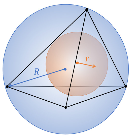
Figure 2.
Tetrahedron with the inradius r and the circumradius R, respectively, drawn in orange and blue.
The factor 3 is used to normalize the value of q in the range . For a regular tetrahedron, q equals 1; therefore, a good-quality mesh should have most of tetrahedra with quality index close to 1.
4. Dosimetric Models
To make a fair comparison between the results obtained with voxel and tetrahedral meshes, it is important to remove possible geometric inconsistencies. For this reason, the tetrahedral mesh is first created with a commercial software setting a uniform mesh size. Then, starting from this tetrahedral mesh, a regular cubic discretization with the desired resolution ( or in this paper) is generated from the terahedral mesh. Each voxel is assigned the same tissue type of the tetrahedron containing the barycenter of the voxel. In this way, the tetrahedral and voxel-based meshes are as similar as possible.
4.1. Multilayered Sphere
The first model used in this paper is a multilayered sphere. The advantage of this model is that it is possible to define an analytical solution taken as reference to compare the numerical results. Figure 3 shows the voxel-based mesh and the tissue type assigned to each layer. Table 1 reports the details about the geometry and the tissue properties.
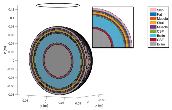
Figure 3.
Multilayered sphere. The various layers are highlighted by different colors. In the inset the stair-casing effect due to the voxel-discretization is displayed. The source field is created by a coil with a radius and located above the center of sphere.

Table 1.
Multilayered sphere structure.
4.2. Human Head—Anatomical 3D Model
Voxel and tetrahedral discretizations are compared considering a more challenging model, the realistic human adult head Colin27 Average Brain (also known as Average Colin). Average Colin is an adult brain atlas [30] that consists of four tissues: skull, cerebrospinal fluid (CSF), gray matter (GM) and white matter (WM). This atlas was obtained by scanning the brain of Colin J. Holmes 27 times (hence the name Colin27) over the course of a few months. The images were combined to create an average brain with high structure definition. The tetrahedral mesh was created by Qianqian Fang (more information can be found in [31]) and it is freely available for download [32]. The model is shown in Figure 4a.
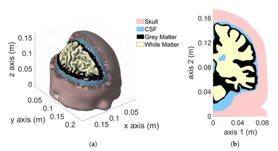
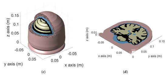
Figure 4.
Colin27 Average Brain: 3D model (a), 2D cut-plane (b), axisymmetric model (c) and planar model (d).
The following tissue conductivities are used: skull , cerebrospinal fluid , grey matter and white matter . The operating frequency is .
4.3. Human Head—Simplified 3D Models
To highlight the source of numerical artifacts, before considering the complete 3D model described in Section 4.2, two simplified 3D models were created. The first model is obtained by rotating a cutplane of Colin27 average brain (Figure 4b) along the longitudinal axis (axis 2 of the figure) by . The result is the axisymmetric model represented in Figure 4c. In this case, a uniform vertical magnetic field is used as the source. The second model is obtained by mirroring the cutplane of Figure 4b with respect to the sagittal plane and extruding the result by a thickness of along the z-axis. The result is the 3D representation of a planar geometry reported in Figure 4d. An impressed external field parallel to the extrusion direction is considered as source. The added value of these simplified models is that they can be simulated as 2D axisymmetric and 2D planar problems. The 2D solutions obtained with a very fine mesh are used as reference for the 3D simulations, making it possible to investigate and understand the causes of the numerical artifacts. The mesh related to the 2D head models has been manually tuned in order to achieve accurate results without the need for any filtering of the raw solution. For instance, all sharp edges were pre-processed with an automated program, imposing a minimum curvature radius of between each of the adjacent boundary edges, as shown in Figure 5.
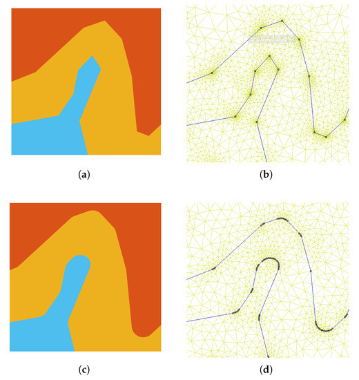
Figure 5.
Manual control of the tetrahedral mesh: the boundaries were smoothed to avoid singularities. Tissue boundaries before local smooth edits (a) and the related mesh (b). Tissue boundaries after local smooth edits (c) and the related mesh (d).
5. Numerical Results
5.1. Multilayered Sphere
The multilayered sphere is exposed to the magnetic flux density generated by a coil with a radius of that is located above the center of the sphere, as shown in Figure 3. The axis of the coil is the z-axis and the origin of the reference system corresponds to the center of the sphere. The operating frequency is and the current flowing through the coil is .
The induced electric field is computed using the numerical method described in Section 2 for both tetrahedral and voxel-based mesh. In the tetrahedral mesh, the number of nodes is about 323,600 and of tetrahedra is 1,883,300. The corresponding voxel mesh is generated using for the voxel side. This results in a model with about 2,205,000 nodes and 2,144,100 voxels. It is crucial to observe that the symmetry of the exposure scenario forces the induced currents to circulate within a single tissue. Consequently, hot spots due to field singularity and/or high contrast between conductivities of contiguous tissues are avoided. Therefore, the only source of numerical artifacts in this case is the stair-casing approximation (for the voxel mesh).
Table 2 shows the maximum value of the electric field in each tissue for the analytical solution. The common post-processing method of the numerical results coming from a voxel model involves the application of specific metrics to remove numerical artifacts. The analysis and comparison of the different filtering metrics are beyond the scope of this paper. The underlying idea behind all techniques is to remove the hot spots of the electric field due to numerical artifacts. To this aim, the ICNIRP guidelines propose to consider the 99th percentile [5]. However, many authors point out that in the case of localized exposure, considering the 99th percentile can underestimate the actual maximum induced field [22,33]. To overcome this issue, the th percentile is sometimes preferred [3,15]. Other techniques, based on statistical considerations rather than on arbitrary thresholds, remove the outliers in the distribution of the induced electric fields [6,7] in a post-processing operation, or try to prevent them by smoothing the contrast of conductivities between adjacent tissues [6,22]. In this paper, the maximum value obtained in the raw data is presented together with the th and the 99th percentile. For the tetrahedral mesh only the maximum value is presented. To better appreciate the deviation from the analytical solution, each value obtained in the numerical simulations is divided by the related analytical reference value. Due to the properties of the exposure scenario, the maximum exposure is registered in the outermost layer (skin). In this tissue, in the voxel mesh the maximum value overestimates the exposure by 15%, the 99.9th percentile overestimates the exposure by 5% and the 99th percentile underestimates the exposure by 2%. Using the tetrahedral mesh, without any filtering metric, the maximum deviation is 0.5%.
Table 2.
Deviation between analytical and computed induced electric field on tetrahedral and voxel-based mesh.
5.2. Human Head—Simplified 3D Model
Several exposure scenarios were studied for the two simplified 3D head models, all leading to the same conclusions. Therefore, for the sake of shortness, only the exposure to a homogeneous magnetic flux density is presented. The value of , corresponding to the reference level for public exposure is considered [5]. In both axisymmetric and planar cases (Figure 4c,d, respectively), the magnetic flux density has only z-component.
Three-dimensional models corresponding to the axisymmetric and planar cases were created with both voxel ( and side) and tetrahedral elements to perform 3D simulations. For a fair comparison, tetrahedral meshes are created using a uniform mesh size such that the average volume of tetrahedra was equal to .
Table 3 summarizes the results for the axisymmetric case. First, it is worth stressing that, for the symmetry of the problem, as in the case of the multilayered sphere, the only source of numerical artifacts is the stair-casing approximation. The maximum exposure is registered in the skull and the tetrahedral mesh makes it possible to determine the maximum exposure without filtering the raw data with a maximum deviation of 0.2% with respect to the reference solution.
Table 3.
Deviation of the E-field in the axisymmetric case.
Different conclusions can be drawn for the planar case. In this case, in fact, the induced currents cross the tissue boundaries, hence, possible numerical artifacts are not limited only to staircasing. Field singularities and the contrast of conductivities between contiguous tissues cause numerical artifacts as well. For this reason, the results of the planar case summarized in Table 4 appear completely different. The maximum exposure is registered in the gray matter and, in this tissue the use of tetrahedral elements causes an underestimation of about 7%. In the same tissue, the underestimation caused by the use of voxel elements is even higher, up to 50% when the 99th percentile is applied.
Table 4.
Deviation of the E-field in the planar case.
5.3. Human Head—Complete 3D Model
In this section, exposure of a realistic head model is considered in two scenarios: (1) homogeneous magnetic flux density with a single component in the z-direction of , (2) magnetic flux density created by a coil with a radius of . The coil lays in the plane and the distance from the head is . The center of the coil is aligned with the head center and the current flowing in the coil is . The induced electric field is computed using tetrahedral and voxel elements. In the tetrahedral mesh is the original available in [32] without additional refinement, containing about 70,200 nodes and 423,400 tetrahedra; in the voxel mesh there are about 4,140,000 nodes and 4,045,000 elements when the resolution is , and about 32,753,000 nodes and 32,374,000 elements when the resolution is .
Results are provided in terms of maximum value, th percentile and 99th percentile for both voxel and tetrahedra in Table 5 (homogeneous case) and in Table 6. The induced electric field exhibits higher values in the skull and gray matter. A graphical comparison for the case of localized exposure scenario in several tissues is shown in Figure 6. The maps of the electric field for all meshes are in good agreement.
Table 5.
Deviation of the E-field in the homogeneous case—all values are expressed in mV/m.
Table 6.
Deviation of the E-field in the localized case—all values are expressed in mV/m.
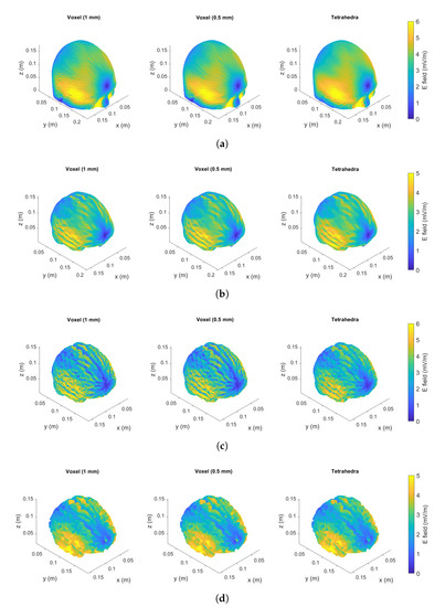
Figure 6.
Localized exposure (coil in front of the head model). The induced electric field in Colin27 Average Brain is shown for tetrahedral mesh and voxel-based meshes with resolution of e in each tissue: skull (a), CSF (b), grey matter (c) and white matter (d).
In the case of homogeneous exposure, Table 5, it is possible to observe that the maximum value obtained with the tetrahedral mesh is always lower than the one obtained with voxels. However, when moving to the more realistic localized exposure this result is not confirmed for all tissues. In the cerebrospinal fluid (CSF) and white matter (WM) the tetrahedral elements lead to the highest maximum value of induced electric field. This means that, when staircasing is not the only source of numerical artifacts, tetrahedral meshes are also subject to numerical artifacts.
To better understand the causes of the peak values obtained within the tetrahedral mesh, a correlation with the quality index q is carried out. First of all, the overall mesh quality is shown in Figure 7. It is possible to observe that most of the tetrahedral elements have an acceptable quality index (). However, elements with a low quality index exist. The quality index q related to the tetrahedron with the maximum electric field value is equal to in the cerebrospinal fluid (see Figure 8a), while it is equal to in the white matter (see Figure 8b). This means that, while in the white matter the “culprit” for the numerical artifact is likely to be the irregular shape of the tetrahedron, the same conclusion does not apply to the CSF tissue. In fact, the maximum value in the CSF is related to a tetrahedron belonging to the boundary characterized by a high conductivity contrast ( in the CSF, in the neighbor tissues). In this case, the induced currents cross tissue boundaries causes numerical artifacts due to the large difference in conductivities between adjacent tissues (tissue contrast). By applying the th and 99th percentile to all meshes, the results are in a good agreement (i.e., the deviation is fully within the uncertainty related to the tissue properties). Therefore, the most suitable metric can be selected according to the most recent literature on the subject [3,6,7] and they should be applied also to the results obtained using a tetrahedral mesh.
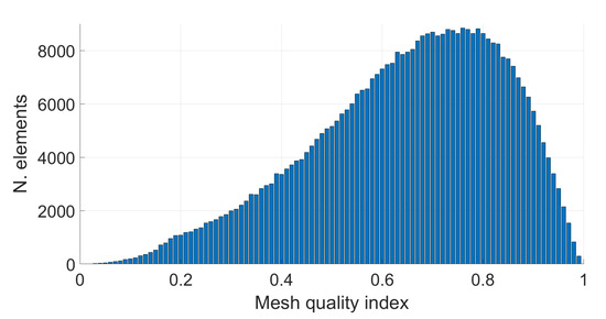
Figure 7.
Tetrahedral mesh quality of Colin27 3D model. The quality index is on the x-axis, while the number of tetrahedral elements corresponding to the respective mesh quality index is shown on the y-axis.
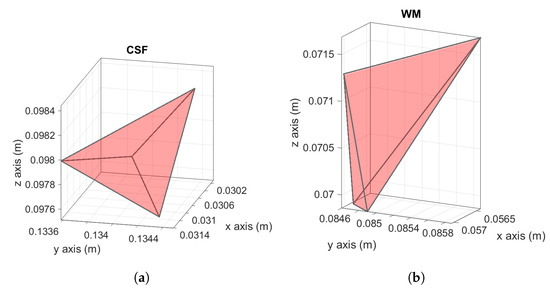
Figure 8.
Tetrahedron with related to the maximum electric field in CSF (a). Tetrahedron with related to the maximum electric field in the white matter (b).
6. Conclusions
Several exposure scenarios were analyzed in order to study whether tetrahedral meshes were capable of suppressing numerical errors caused by stair-casing approximation errors in voxelized models when curved boundaries are approximated with voxels. From the analysis, we discovered that both voxelized and tetrahedral head models suffered from artifacts in the evaluation of high electric field values. In [15], a similar conclusion was obtained but the cause of the artifacts was mainly associated with the presence of low quality tetrahedra.
In this paper, we showed that a tetrahedral mesh is indeed able to remove the source of computational artifacts related to the geometrical modeling of the computational domain (stair-casing), however, in a real exposure scenario, other sources of numerical artifacts are still present. These numerical artifacts are related to two fundamental factors: tetrahedral mesh quality and tissue contrast effect. It was shown that the conductivity contrast between neighboring tissues can cause very high electric fields even in tetrahedra with good quality index. For this reason, even when the mesh quality is close to ideal, it is almost impossible to avoid the crossing of induced currents across tissue interfaces in real exposure scenarios. As a consequence, the use of filtering techniques cannot be completely avoided.
Author Contributions
Conceptualization, F.F., L.G. and R.S.; Formal analysis, A.C.G.; Investigation, A.C.G.; Software, F.F., L.G. and R.S. All authors have read and agreed to the published version of the manuscript.
Funding
This research received no external funding.
Institutional Review Board Statement
Not applicable.
Informed Consent Statement
Not applicable.
Data Availability Statement
Not applicable.
Conflicts of Interest
The authors declare no conflict of interest.
References
- Reilly, J.P.; Hirata, A. Low-frequency electrical dosimetry: Research agenda of the IEEE International Committee on Electromagnetic Safety. Phys. Med. Biol. 2016, 61, R138–R149. [Google Scholar] [CrossRef] [PubMed]
- Hirata, A.; Diao, Y.; Onishi, T.; Sasaki, K.; Ahn, S.; Colombi, D.; De Santis, V.; Laakso, I.; Giaccone, L.; Joseph, W.; et al. Assessment of Human Exposure to Electromagnetic Fields: Review and Future Directions. IEEE Trans. Electromagn. Compat. 2021, 63, 1619–1630. [Google Scholar] [CrossRef]
- Diao, Y.; Gomez-Tames, J.; Rashed, E.A.; Kavet, R.; Hirata, A. Spatial Averaging Schemes of In Situ Electric Field for Low-Frequency Magnetic Field Exposures. IEEE Access 2019, 7, 184320–184331. [Google Scholar] [CrossRef]
- Christ, A.; Kainz, W.; Hahn, E.; Honegger, K.; Zefferer, M.; Neufeld, E.; Rascher, W.; Janka, R.; Bautz, W.; Chen, J.; et al. The Virtual Family – development of surface-based anatomical models of two adults and two children for dosimetric simulations. Phys. Med. Biol. 2010, 55, 23–38. [Google Scholar] [CrossRef]
- Lin, J.; Saunders, R.; Schulmeister, K.; Soderberg, P.; Stuck, B.E.; Taki, M.; Veyret, B.; Ziegelberger, G.; Swerdlow, A.; Repacholi, M.H.; et al. ICNIRPGuidelines for limiting exposure to time-varying electric and magnetic fields (1 Hz–100 kHz). Health Phys. 2010, 99, 818–836. [Google Scholar] [CrossRef]
- Gomez-Tames, J.; Laakso, I.; Haba, Y.; Hirata, A.; Poljak, D.; Yamazaki, K. Computational Artifacts of the In Situ Electric Field in Anatomical Models Exposed to Low-Frequency Magnetic Field. IEEE Trans. Electromagn. Compat. 2018, 60, 589–597. [Google Scholar] [CrossRef]
- Arduino, A.; Bottauscio, O.; Chiampi, M.; Giaccone, L.; Liorni, I.; Kuster, N.; Zilberti, L.; Zucca, M. Accuracy Assessment of Numerical Dosimetry for the Evaluation of Human Exposure to Electric Vehicle Inductive Charging Systems. IEEE Trans. Electromagn. Compat. 2020, 1–12. [Google Scholar] [CrossRef]
- Siauve, N.; Nicolas, L.; Vollaire, C.; Nicolas, A.; Vasconcelos, J. Optimization of 3-D SAR distribution in local RF hyperthermia. IEEE Trans. Mag. 2004, 40, 1264–1267. [Google Scholar] [CrossRef]
- Scorretti, R.; Burais, N.; Fabregue, O.; Nicolas, A.; Nicolas, L. Computation of the Induced Current Density Into the Human Body Due to Relative LF Magnetic Field Generated by Realistic Devices. IEEE Trans. Mag. 2004, 40, 643–646. [Google Scholar] [CrossRef]
- Scorretti, R.; Burais, N.; Nicolas, L.; Nicolas, A. Modeling of induced current into the human body by low-frequency magnetic field from experimental data. IEEE Trans. Mag. 2005, 41, 1992–1995. [Google Scholar] [CrossRef]
- Scorretti, R.; Sabariego, R.V.; Morel, L.; Geuzaine, C.; Burais, N.; Nicolas, L. Computation of Induced Fields Into the Human Body by Dual Finite Element Formulations. IEEE Trans. Mag. 2012, 48, 783–786. [Google Scholar] [CrossRef][Green Version]
- Fang, Q.; Boas, D.A. Tetrahedral mesh generation from volumetric binary and grayscale images. In Proceedings of the 2009 IEEE International Symposium on Biomedical Imaging: From Nano to Macro, Boston, MA, USA, 28 June–1 July 2009; pp. 1142–1145. [Google Scholar]
- Lelong, T.; Tang, Z.; Scorretti, R.; Thomas, P.; Le Menach, Y.; Creusé, E.; Piriou, F.; Burais, N.; Miry, C.; Magne, I. Error estimation in the Computation of Induced Current of Human Body in the Case of Low frequency Magnetic Field Excitation. In Proceedings of the Compumag 2013, Budapest, Hungary, 30 June–4 July 2013; p. PC1-11. [Google Scholar]
- Hoang, L.H.; Scorretti, R.; Burais, N.; Voyer, D. Numerical Dosimetry of Induced Phenomena in the Human Body by a Three-Phase Power Line. IEEE Trans. Mag. 2009, 45, 1666–1669. [Google Scholar] [CrossRef]
- Soldati, M.; Laakso, I. Computational errors of the induced electric field in voxelized and tetrahedral anatomical head models exposed to spatially uniform and localized magnetic fields. Phys. Med. Biol. 2020, 65, 015001. [Google Scholar] [CrossRef] [PubMed]
- Dawson, T.; Stuchly, M. Analytic validation of a three-dimensional scalar-potential finite-difference code for low-frequency magnetic induction. Appl. Comput. Electrom. 1996, 11, 72–81. [Google Scholar]
- So, P.; Stuchly, M.; Nyenhuis, J. Peripheral nerve stimulation by gradient switching fields in magnetic resonance imaging. IEEE Trans. Biomed. Eng. 2004, 51, 1907–1914. [Google Scholar] [CrossRef]
- Dimbylow, P. Development of the female voxel phantom, NAOMI, and its application to calculations of induced current densities and electric fields from applied low frequency magnetic and electric fields. Phys. Med. Biol. 2005, 50, 1047–1070. [Google Scholar] [CrossRef]
- Hirata, A.; Takano, Y.; Kamimura, Y.; Fujiwara, O. Effect of the averaging volume and algorithm on the in situ electric field for uniform electric- and magnetic-field exposures. Phys. Med. Biol. 2010, 55, N243–N252. [Google Scholar] [CrossRef]
- Canova, A.; Freschi, F.; Giaccone, L.; Repetto, M. Exposure of working population to pulsed magnetic fields. IEEE Trans. Magnet. 2010, 46, 2819–2822. [Google Scholar] [CrossRef]
- Zoppetti, N.; Andreuccetti, D.; Bellieni, C.; Bogi, A.; Pinto, I. Evaluation and characterization of fetal exposures to low frequency magnetic fields generated by laptop computers. Progress Biophys. Mol. Biol. 2011, 107, 456–463. [Google Scholar] [CrossRef]
- Laakso, I.; Hirata, A. Reducing the staircasing error in computational dosimetry of low-frequency electromagnetic fields. Phys. Med. Biol. 2012, 57, N25–N34. [Google Scholar] [CrossRef]
- Canova, A.; Freschi, F.; Giaccone, L.; Manca, M. A Simplified Procedure for the Exposure to the Magnetic Field Produced by Resistance Spot Welding Guns. IEEE Trans. Magn. 2016, 52, 1–4. [Google Scholar] [CrossRef]
- Freschi, F.; Giaccone, L.; Cirimele, V.; Canova, A. Numerical assessment of low-frequency dosimetry from sampled magnetic fields. Phys. Med. Biol. 2018, 63, 015029. [Google Scholar] [CrossRef] [PubMed]
- Notay, Y. AGMG. Version 3.3.5. 2022. Available online: http://agmg.eu/ (accessed on 24 June 2022).
- Notay, Y. An aggregation-based algebraic multigrid method. Electron. Trans. Numer. Anal. 2010, 37, 123–146. [Google Scholar]
- Napov, A.; Notay, Y. An Algebraic Multigrid Method with Guaranteed Convergence Rate. SIAM J. Sci. Comput. 2012, 34, A1079–A1109. [Google Scholar] [CrossRef]
- Notay, Y. Aggregation-Based Algebraic Multigrid for Convection-Diffusion Equations. SIAM J. Sci. Comput. 2012, 34, A2288–A2316. [Google Scholar] [CrossRef]
- Field, D.A. Qualitative measures for initial meshes. Int. J. Numer. Methods Eng. 2000, 47, 887–906. [Google Scholar] [CrossRef]
- Collins, D.L.; Zijdenbos, A.P.; Kollokian, V.; Sled, J.G.; Kabani, N.J.; Holmes, C.J.; Evans, A.C. Design and construction of a realistic digital brain phantom. IEEE Trans. Med. Imaging 1998, 17, 463–468. [Google Scholar] [CrossRef]
- Fang, Q. Mesh-based Monte Carlo method using fast ray-tracing in Plucker coordinates. Biomed. Opt. Express 2010, 1, 165–175. [Google Scholar] [CrossRef]
- Colin27 Adult Brain Atlas FEM Mesh. Available online: http://mcx.space/wiki/index.cgi?MMC/Colin27AtlasMesh (accessed on 24 June 2022).
- Chen, X.L.; Benkler, S.; Chavannes, N.; Santis, V.D.; Bakker, J.; van Rhoon, G.; Mosig, J.; Kuster, N. Analysis of human brain exposure to low-frequency magnetic fields: A numerical assessment of spatially averaged electric fields and exposure limits. Bioelectromagnetics 2013, 34, 375–384. [Google Scholar] [CrossRef]
Publisher’s Note: MDPI stays neutral with regard to jurisdictional claims in published maps and institutional affiliations. |
© 2022 by the authors. Licensee MDPI, Basel, Switzerland. This article is an open access article distributed under the terms and conditions of the Creative Commons Attribution (CC BY) license (https://creativecommons.org/licenses/by/4.0/).