Article

Intelligent Manufacturing Planning System Using Dispatch Rules: A Case Study in Roofing Manufacturing Industry

1
Department of Computer Science and Embedded Systems, Faculty of Computing and Information Technology, Tunku Abdul Rahman University College, Kuala Lumpur 53300, Malaysia
2
Institute of IR4.0, Universiti Kebangsaan Malaysia, Bangi 43600, Malaysia
3
GMCM Sdn. Bhd., Seri Kembangan 43300, Malaysia
4
Faculty of Data Science and Information Technology, Inti International University, Nilai 71800, Malaysia
*
Author to whom correspondence should be addressed.
Appl. Sci. 2022, 12(13), 6499; https://doi.org/10.3390/app12136499
Submission received: 25 May 2022 / Revised: 17 June 2022 / Accepted: 18 June 2022 / Published: 27 June 2022
(This article belongs to the Special Issue Innovations in Intelligent Machinery and Industry 4.0)

Abstract

:
This paper aims to investigate the optimal sorting of orders reflecting on the material changing lead time over the machines in the roofing manufacturing industry. Specifically, a number of jobs were sorted together based on the material used and then consolidated for subsequent processes, i.e., assigned to the corresponding machines. To achieve the optimal sorting for the received orders, a combinatorial dispatch rule was proposed, which were Earliest Due Date (EDD), First In First Out (FIFO), and Shortest Processing Time (SPT). The sequence of orders organized by the scheduling algorithm was able to minimize the changing material lead time and also maximize the number of orders to be scheduled in the production. Consequently, on-time delivery could be achieved. Tests based on real data have been set up to evaluate the performance of the proposed algorithm in sorting the received orders. As a result, the proposed algorithm has successfully reduced the material changing lead time by 47.3% and 40% in the first and second tests, respectively.

1. Introduction

In the era of the Fourth Industrial Revolution, many countries aspire to embrace the digital transformation of manufacturing or production plants. However, many Small and Medium Industries (SMI) or Small and Medium Enterprises (SME) are not ready for the industrial revolution, especially in Malaysia [1]. In recent years, there are many Industry 4.0-related programs and incentives offered by the government, such as the Readiness Assessment, Intervention Fund, Domestic Investment Fund (DISF), and Automation Capital Allowance (Automation CA), with the aim of assisting the SMIs and SMEs to work towards Industry 4.0 [2]. Industry 4.0 growth is inevitable and may impact the traditional business manufacturing industry that is labor-intensive and cost-sensitive [3]. In fact, market demand is very dependent on the economic conditions, the rise of new markets, and product diversity [4]. The integration of planning and scheduling not only satisfies customers’ requirements but also optimizes the resources and achieves on-time delivery. Insufficient modal and lack of advanced technology are some of the main reasons that many old players in the industry resist the digital transformation [5]. First of all, when SMEs begin the transition to Industry 4.0, they refuse to start from scratch, and secondly, SMEs tend to become overwhelmed by the multitude of technologies that are currently available on the market [6]. Ultimately, most of the processes in the manufacturing industry are similar as in Figure 1.
Figure 1 shows a simple process of production. It shows that proper production planning is important because each step of the process affects the others. In conjunction with this, the main goal of production planning is to achieve high customer satisfaction with a low cost [8]. Production planning can be divided into the product structure, material requirement planning, and uncertainty management [9]. As the customer demand is increasing, the manufacturers realize that most of them are facing the same problem in the production stage. This resulted in the emergence of modern production planning tools and methods in the late 19th century.
In the past, traditional manufacturing systems focused on reducing cost and improving efficiency. However, they have not been able to follow the current trends, such as agile manufacturing, networked manufacture, mass customization, intelligent manufacture, and et cetera [10]. In fear of being eliminated by the competitors, a lot of SMIs and SMEs were forced to transform their business model. The transformation allowed them to cater to fluid customer demand. However, their demands may change often and dramatically in some cases [11].
Resource limitation is one of the common challenges. Hence, scheduling is essential to handle the allocation of resources based on the job sequence [12]. The output of the schedules is a production plan to estimate the start and end times for every job and machine. The jobs are planned according to certain optimization criteria while the scheduling performance is evaluated based on performance indicators such as costs, resource utilization, and adherence to deadlines. To strengthen the competitiveness of Malaysia as a production location, the manufacturing industry has to respond quickly and more flexibly according to the business models.
The objectives of production planning are to reduce inventory levels, increase machine utilization, and improve customer responsiveness [13]. Based on these objectives, many manufacturers are willing to provide customization services to improve customers’ satisfaction [14]. For example, Make-To-Order (MTO) is a business model that refers to a just-in-time philosophy due to the zero-inventory level between the stage of production and distribution [15]. This is to cater to personal customization, as shown in Figure 2.
Due to the different requirements of every customer, production has to produce products according to the needs of the customer. In this situation, productivity is restricted due to the maximum capacity of each machine. This is where material management plays an important role in production. When a manufacturing process has ended for one order, the next order may require another raw material. This may cause a long changing material lead time, as the operator has to request the raw material needed, and then perform material handling until the machine is set up.
Besides that, the complexity of sorting the orders at the stage of production planning will be higher due to the different order and delivery dates set by the customers. This may also affect the on-time delivery. It is difficult to achieve sorting optimization with so many different parameters in the production planning phase, such as time, product quality, and profit. Moreover, the performance of production planning will be inconsistent due to human involvement. Figure 2 shows the manual production planning:
Traditionally, once a customer makes an order, the order is submitted to the production office. The production office personnel manually assign the material according to the customer’s request based on experience. Then, those orders are sent to the planner to arrange the production schedule. However, each order is printed out as a hard copy. If there are any amendments, they are recorded on the hard copy, which is inconvenient. From the system layer point of view, the process of the data transfer still requires human involvement.
The optimization of production scheduling is viewed as a complicated task. Therefore, most of the schedulers prefer to employ simulation-based software or a manual decision-making process [16]. In this work, we integrated domain expert knowledge to generate the decisions. Priority dispatching rules were used for production planning, such as First-in-First Out (FIFO), Shortest Processing Time (SPT), and Earliest Due Date (EDD). The main objective of this research is to achieve sorting optimization in order to reduce the material changing lead time in the production and also to achieve On-Time Delivery expectations by customers. We adopted the methodology proposed by [17] in the case study of the roofing manufacturing industry. Oluyisola et al. proposed the following steps:
  • Step 1. Preliminary study.
  • Step 2. System requirements specification.
  • Step 3. Identify data sources and choose relevant analytics that fits the problem.
  • Step 4. Design system and data architecture with consideration for integration with extant systems.
  • Step 5. Implement with considerations for development methodologies, continuous innovation, and long-term adaptability.
Based on the aforementioned objective, the main contribution of our work is to implement a digital transformation on the legacy machines in the roofing manufacturing industry. This is a case study that used real data, and which, in the near future, can be generalized to a large-scale project.

2. Related Work

2.1. An Overview of SMIs and SMEs in Malaysia

According to the World Bank, approximately 98.5% of the business establishments in Malaysia are SMEs, which proves the importance of SMEs in Malaysia [18]. However, they are lacking resources in some respects, such as talent, funds, and technology. Table 1 shows the definition of SMEs in Malaysia.
The definition of the SME in Malaysia was reviewed in 2013. Lately, it was endorsed during the 14th NSDC Meeting in July 2013, and all sectors were covered. Table 1 shows that SMEs are defined as a company with a sales turnover that is not more than RM50 million or where the maximum number of full-time employees is 200 people in the manufacturing sector. Besides that, for the services and other sectors, SMEs are defined as the company’s sales turnover, not more than RM20 million, or the number of full-time employees not more than 75 people. Due to the ever-changing market demand, it will be incredibly challenging for SMEs to adopt Industry 4.0 effectively. With the consideration of return-on-investment, some may remain with their existing technology if they can still survive in the moment.

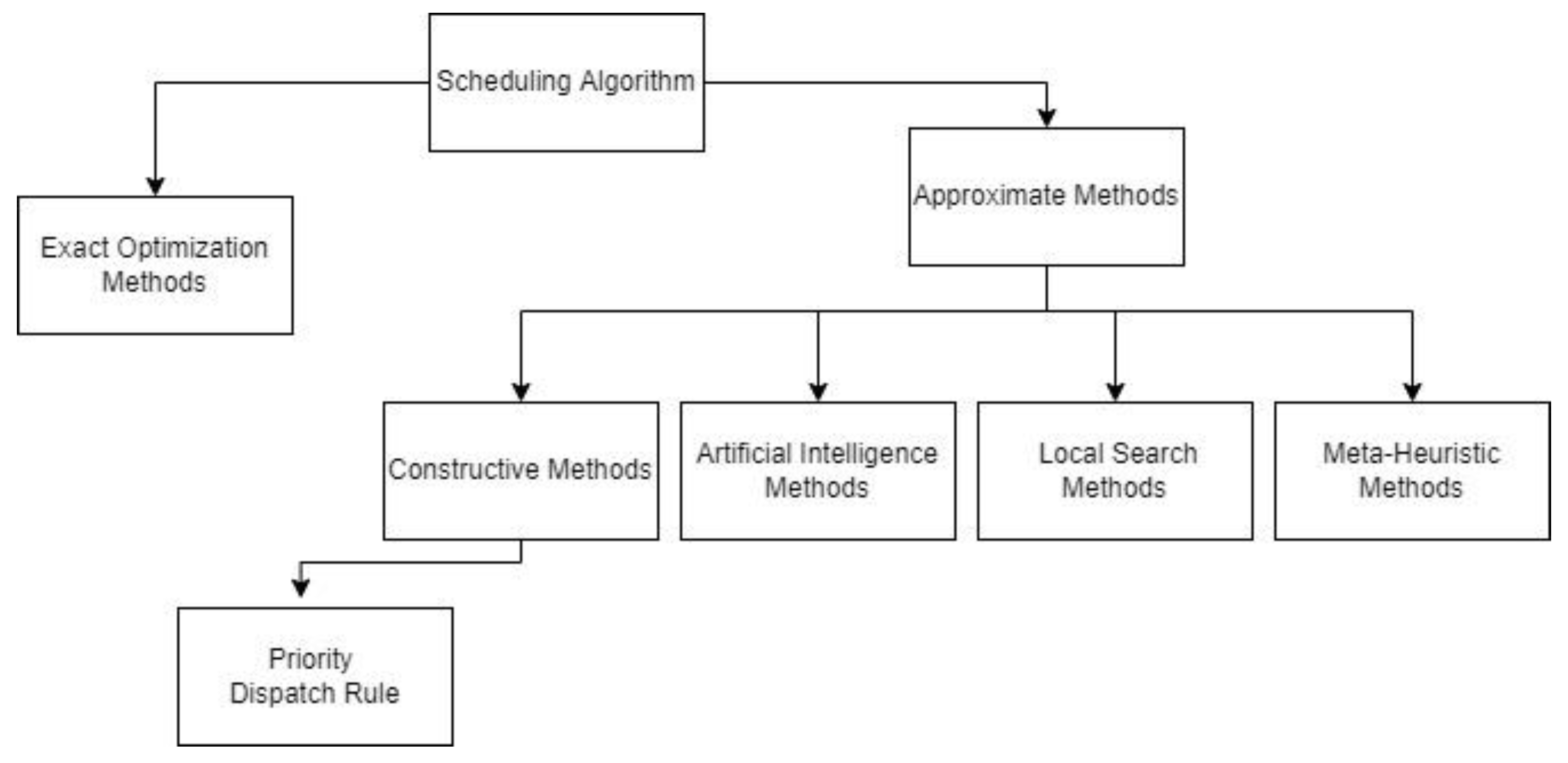
2.2. Optimization Algorithm for Scheduling

Production scheduling needs to send the information to the machine at the shop floor once the orders are scheduled and update the status once the order has been done. There are two major scheduling algorithms, which are the exact optimization methods and the approximate methods. Figure 3 shows an overview of the scheduling algorithms.
The exact optimization methods were applied to solve the scheduling problem from the 1950s to the 1980s. For example, the efficient rule method, the mathematical programming method, and the branch and bound method. As the scheduling problems become more complex, the exact optimization method is not suitable for a practical scheduling problem because it is unable to reach a solution efficiently [21].
The past decade has seen the rapid development of the approximate methods in solving scheduling problems. For example, constructive methods, artificial intelligence methods, local search methods, and meta-heuristic methods.
Generally, the exact optimization algorithm, such as the mathematical programming method and the branch and bound method, are more suitable to solve problems with a small size. In contrast, approximate algorithms such as metaheuristic methods can solve large-scale problems [22]. However, no single approach can solve all Job Shop Scheduling (JSP) problems [23]. Hence, hybrid methods are used for different situations in JSPs.

2.2.1. Artificial Intelligence (AI) Methods, Local Search Methods, and Metaheuristic Methods

Recent advances in AI have enabled intelligent solutions to handle scheduling problems in real-time [24]. However, the AI methods require a distinct cyclical nature that demands constant iteration, tuning, and improvement to find the best solution. The local search method is a greedy methodology used to solve a big combinatorial optimization problem within a reasonable time [25]. As the local search method is very dependent on time, it can achieve optimization if there is sufficient time given. Metaheuristic methods use a set of intelligent strategies to explore and exploit the search base to find the optimal solution [26]. Many metaheuristic methods focus on reducing the makespan in flow shops [27]. The metaheuristic method can solve large and more complex problems than the local search method. Other than that, Chiang et al. [28] applied clustering methods to optimize storage location planning and consolidated picking strategy for 98 orders with a preplanned storage space. This indicates that the time required for local search methods or metaheuristic methods can be saved with the help of domain knowledge.
In summary, AI methods are suitable for dynamic job shops to deal with random job arrivals with unexpected machine breakdowns. Local search methods are more efficient to solve large combinatorial optimization problems, while metaheuristic methods are more efficient to solve larger and more complex optimization problems in a reasonable time frame. These algorithms are usually iteratively learnt and modified to reach the desired result. This may not be suitable to implement in our case study that sorts orders based on their urgency and product customization.

2.2.2. Dispatch Rule Algorithms in Constructive Methods

The constructive method is one of the methods in the approximate methods that solves the JSP efficiently in a dynamic environment [29]. Since production in the roofing industry relies on individual customers [7], i.e., the dynamic environment, constructive methods were utilized for our scheduling algorithm. One of them is the priority dispatch rule. As a priority function, dispatch rules calculate the priority values of the operation so that the operation will process from the job with highest priority [30]. In manufacturing, especially in the roofing industry, the business model is based on the MTO. Hence, our scheduling algorithm consists of a set of priority rules to schedule the jobs to ensure the products are delivered based on the customer’s requirement. Subsequently, customer satisfaction can also be improved.

3. Methods

3.1. Definition

In this work, many items may belong to one order, and each order was assigned to one job J when m machines {M1, M2,…, Mm} were available. Each job requires one machine to complete the process of production at a time. In the development of the production scheduling system, there are a few parameters that require input from users, such as holiday information, shift information, overtime shift information, and machine information. The definition and notation are shown as below:
  • Pi = The processing time for job i;
  • Df = Due date, i.e., the delivery date of the finished goods;
  • STi = Setup time; the time for setup, including material change;
  • Ci = Completion time for job i;
  • Ci = di + Ci,j-1 + Pij (SOi + Pi +STi).
To solve the sorting optimization, reducing the changing material lead time and achieving on-time delivery are essential. There were a few sequencing and scheduling rules used in the algorithm. The Dispatch Rule Algorithms are shown as Table 2.
Some other significant functions used for analysis are as shown below:
  • Makespan time: the length of time that elapses from the start of work to the end.
Mt = Ft − St
  • Setup time: setup time that includes material changing time.
  • Total setup time: the sum of setup time
TSTi = Σ STi

3.2. Assumption

The problem of scheduling normally can be solved by replacing another machine where the factory may have several machines to manufacture the same product. The following assumptions are commonly found in the literature for planning theory:
(1)
Machines are always available and do not break down suddenly.
(2)
Each machine can only process one job at a time.
(3)
No changes are allowed once the schedule is confirmed by the manager.
(4)
Every material data extracted from the ERP System is the latest data.
(5)
Material is always available for production
(6)
All finished goods produced on that date will be delivered to the customer.
(7)
Inputs such as machine detail, holiday detail, shift detail, and machine breakdown detail are keyed in by the user and we expect all the inputs are correct
(8)
Unscheduled orders that have the same due date are postponed to the next day.
(9)
The Application Programming Interface (API) for production sheets only generates confirmed orders.
(10)
All confirmed orders on a selected day belong to a day prior
(11)
The expected setup time including material change is fixed in a time of 15 min
(12)
Machine capacity in a time range from 8 am to 5 pm is 45k square feet.

3.3. Dispatch Rule Algorithms

Dispatch rule algorithms use priority levels to solve JSP problems. For example, First-in-First Out (FIFO), Earliest Due Date (EDD), and Shortest Processing Time (SPT) can be adopted to determine which job is to be executed next during the production stage if there are available machines [31]. Manufacturers are responsible to set their priority level to determine the rules of their own JSP. Previous study has shown that the dispatch rule can perform well when using one or multiple fixed rules in solving the JSP [32,33]. Most of them achieved satisfactory results in their research.
FIFO is the first basic rule in the dispatch rule algorithm. FIFO processes jobs in an orderly manner according to the first arrival of the customer’s order. There were many researchers who used FIFO as the basic rules [34,35,36,37,38,39] due to its simple algorithm. It has no complexity in decision making [40]. For every scheduling algorithm, FIFO can be the baseline algorithm to measure the performance for decision making. EDD arranges the orders according to the Earliest Due Date. Previous research showed that it could improve on-time performance [41,42,43,44]. Lastly, the Shortest Processing Time (SPT) algorithm executes jobs that have the Shortest Processing Time first. A random initialization process can be used by the SPT dispatch rule to optimize the makespan [45]. Besides that, there are many combinatorial dispatch rules that include the SPT as one of the rules in the research, such as [36,39,46,47,48]. When a schedule is constructed based on the SPT dispatch rule, it will arrange the schedule with a random starting point and select the next order with the lowest total processing time and setup time.

3.4. Proposed Method

The proposed methods were designed with consideration for integration with extant systems, as shown in Figure 4. Algorithm A1 was used when only one machine was available, while Algorithm A2 was used for balancing the jobs between two machines.

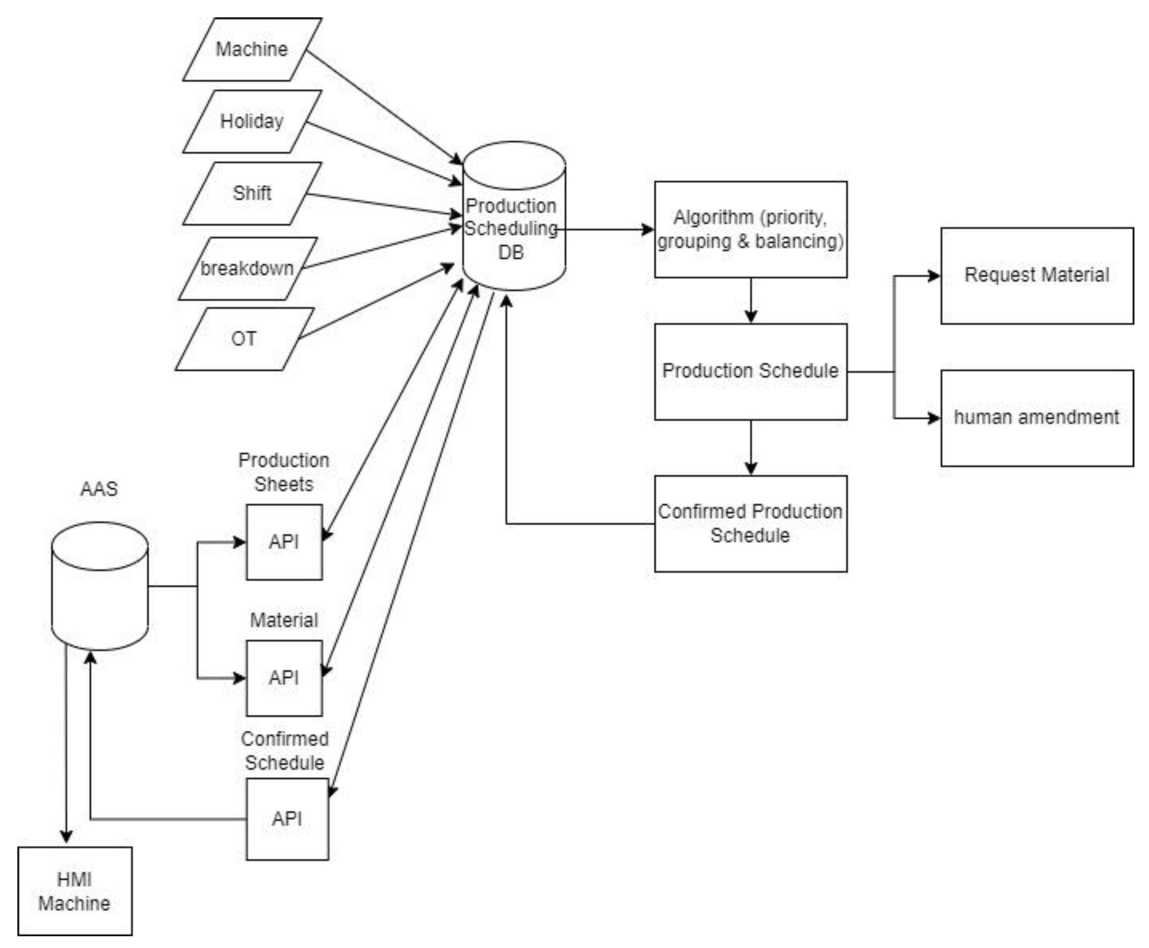
3.4.1. General Data Flow Chart

A general data flow diagram is shown in Figure 4 to illustrate the data flow from the beginning to the end of the planning process.
From Figure 4, there were two different data inputs. The first data input was to gather the input from the user and the second data input was to extract the production sheet information and the material information from the company’s ERP database. For the user input, a group of the parameters were gathered, such as machine information, holiday information, shift information, machine breakdown information, and overtime shift information. The other inputs, such as production sheets and material information, were extracted from the ERP system database through the APIs.
The information gathered was saved in the production scheduling database. Orders would go through the proposed algorithms, as shown in Figure 5, according to the priority level so to create a production schedule. The user selected the material information to determine the materials used in each order. Once the production schedule was confirmed, the production schedule data was then stored in the database and was ready to be sent out to the machine on the shop floor through the APIs. Referring to Appendix A, an ERD diagram of database structure was designed with all the parameters needed.

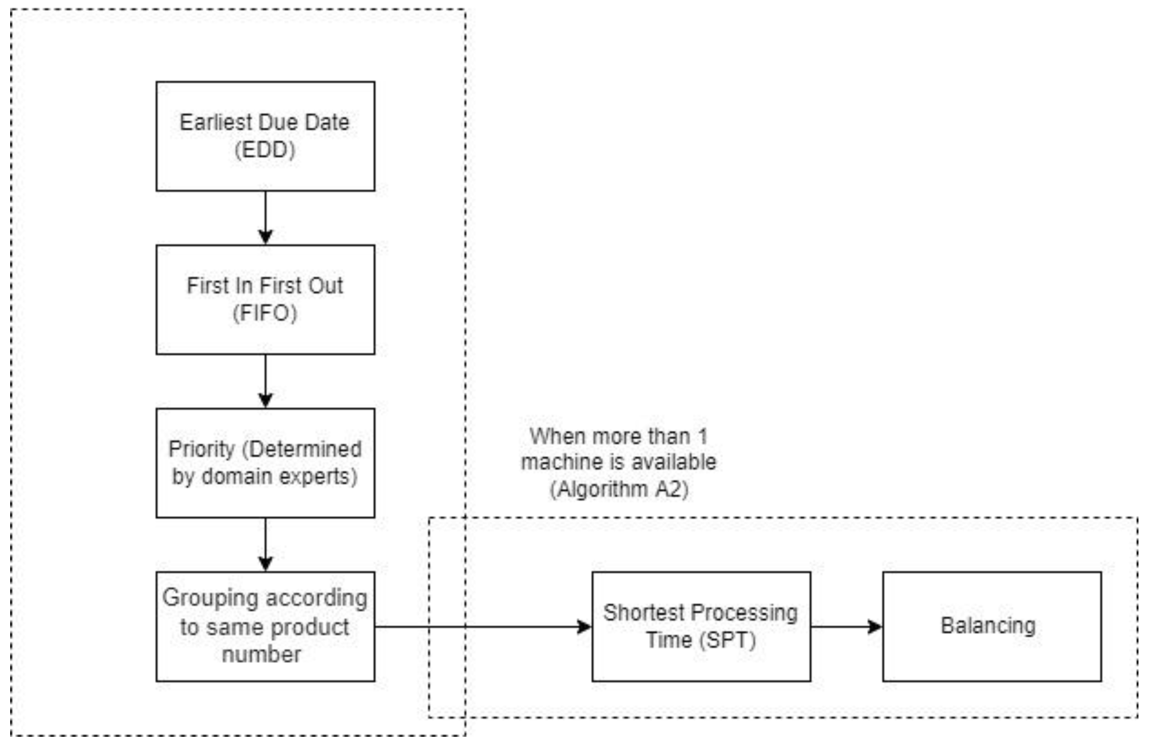
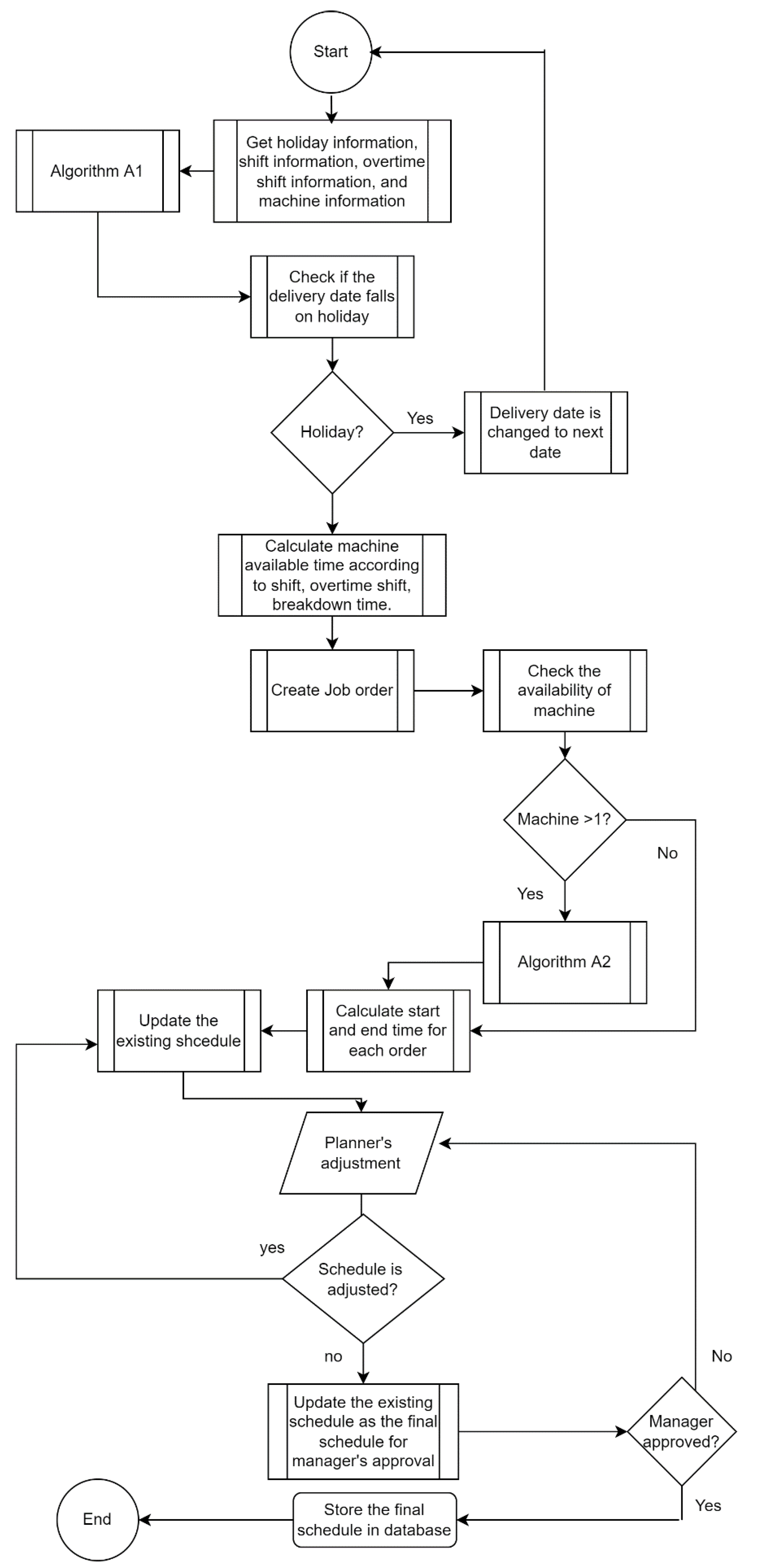
3.4.2. Scheduling Algorithm Flow Chart

The scheduling algorithm flow chart is shown in Appendix A. To minimize the complexity, the schedule must settle the order within one day. When the schedule starts, a date was selected according to the requested date for the orders. Then, all the data were gathered, such as shift information, machine information, and holidays. The orders were sorted based on Algorithm A1 (Appendix B). In our work, the top priority of the scheduling is the requested date, followed by the profile, color, and length. Then, a job order was created.
The requested date was cross-checked with the holiday information. If the delivery date clashed with the holiday, the orders were brought forward to the next day. At the same time, the machine available time was calculated according to the shift information, overtime shift information, and machine breakdown information. Meanwhile, the number of available machines was checked. If there was one machine, the start time and end time were calculated according to the machine’s available time. If there was more than one machine, Algorithm A2 (Appendix C) was executed to do job balancing, followed by the SPT algorithm. Then, only the start time and end time were calculated. This updated schedule was available for planners’ adjustment. Once the planner confirmed the schedule, it was sent to the manager for approval. Lastly, it was stored as the final schedule. The notation of Algorithms A1 and A2 is shown in Table 3.

3.4.3. Algorithm for Optimal Sorting

In Algorithm A1, the dispatch rule algorithms, such as FIFO and EDD, were used. Due to the MTO model, the company has its own priority rule based on the customer’s requirement. Hence, the rule set by the company was arranged in the order of priority by having the requested date as the top priority, followed by color, thickness, profile, and length. Due to the packaging reason, the length was arranged from the longest to the shortest. According to Algorithm A1 in Appendix B, Df is the date that is input by the user. The Df also refers to the delivery date which was requested by customers. At this point, the first rule applied was EDD to extract the orders with the same delivery date. Among these orders, the second rule, i.e., FIFO, was used. Consequently, for Ao, each of the orders was arranged in the FIFO manner, then sorted by using the aforementioned priority rule.
At last, all the orders were grouped based on the production number, in which one production number might have multiple orders that used the same materials. At this point, the total production orders, PO, were arranged by following the SPT rule. This is because the orders which have the same color and thickness were arranged together. The equation of this algorithm is di + Ci,j-1 + Pij.

3.4.4. Balancing Algorithm in Reducing Material Changing Lead Time

Algorithm A2 was used when there was more than one machine available. In this algorithm, SPT and balancing were used to minimize the changing material lead time, which is the setup time. At first, the machine available time was calculated, MAT, and grouped orders, GO, were gathered. To do the balancing, a job was created according to the order, o in GO. Once everything was gathered, the job was assigned to the machine and the job assignment was based on the total number of machines M. While assigning the first job, the system chose the machine k which had the most available time. Algorithm A2 checked the color and thickness against the previous job. If the current job had the same color and thickness, then the job was assigned to the same machine to reduce the changing material lead time. On the other hand, if the color and thickness of the job were different from the previous job, then the current job was assigned to the machine which had the highest available time. This algorithm assigned jobs until the machine ran out of available time.

4. Result and Discussion

Two tests were carried out to evaluate the proposed algorithms. The first test was to evaluate the algorithm on one machine, while the second test was for two machines. The comparison was done in terms of the number of orders and the total setup time before and after the proposed algorithm was implemented. Each test used the same set of orders, which was 87.

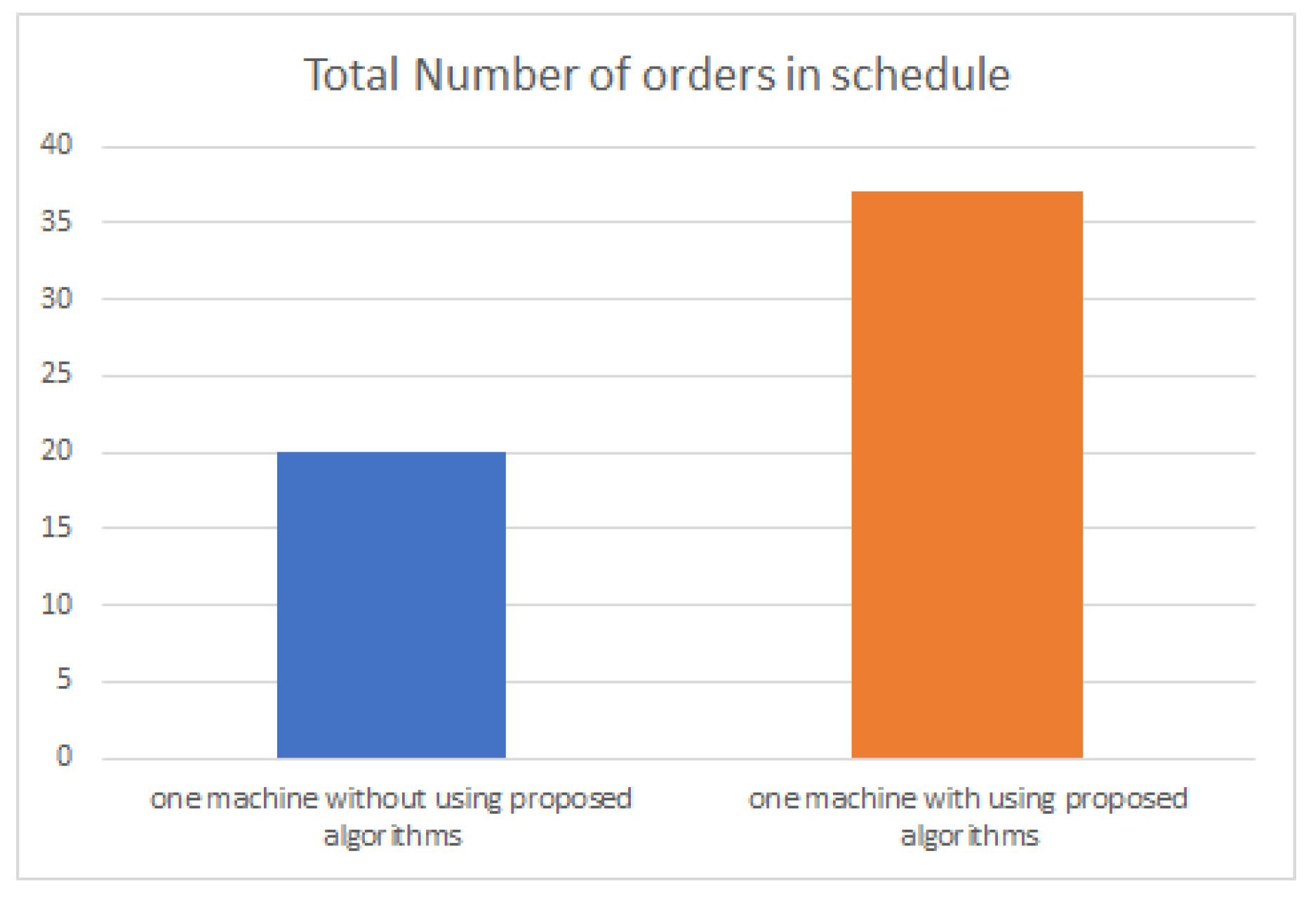
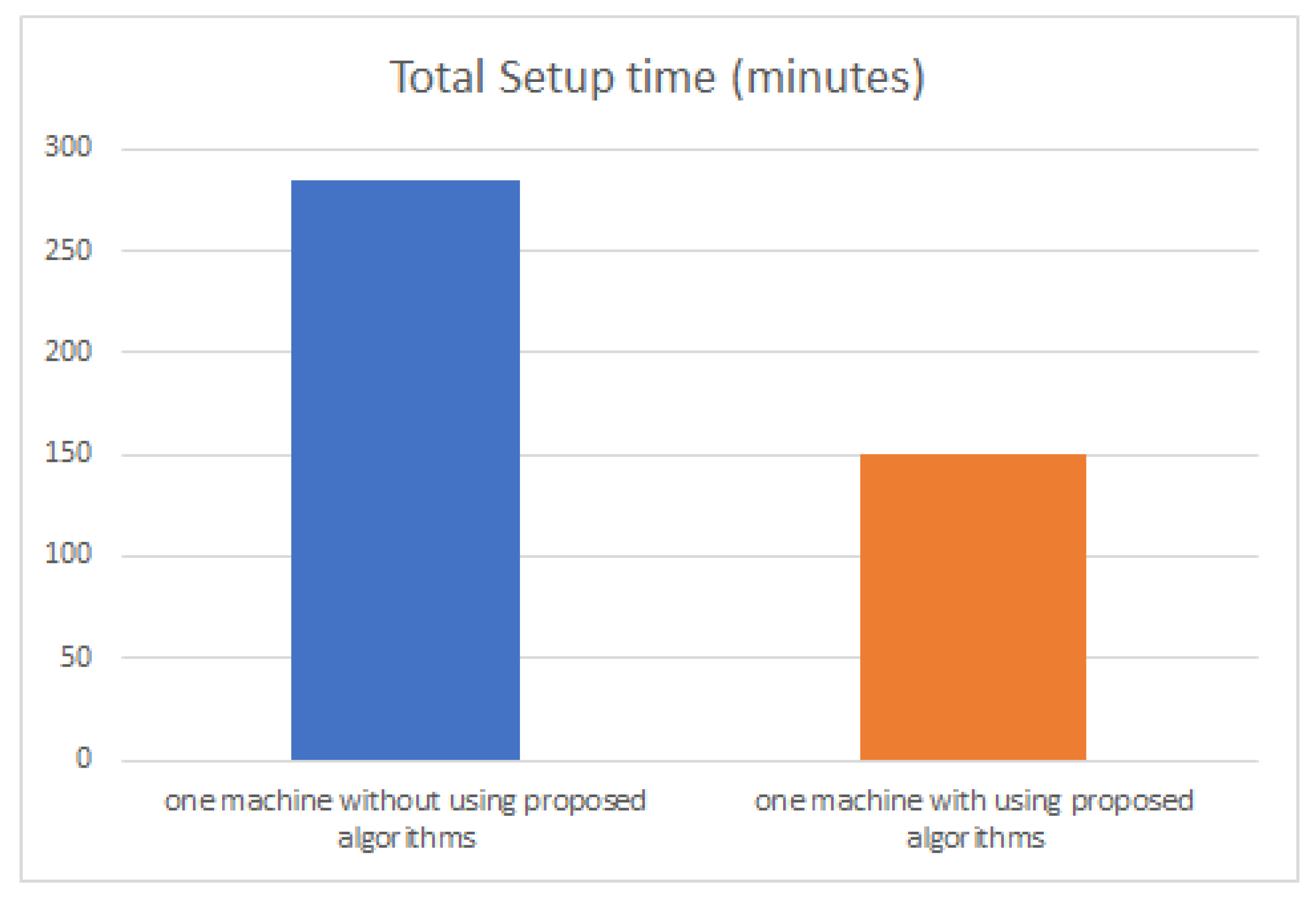
4.1. Result in One Machine Test

The result of using and without using algorithms for only one machine is shown in Table 4. From Table 4, it is seen that more orders could be arranged after using the proposed algorithms.
The performance with and without algorithms in a working day using one machine is shown in Figure 6. The bar chart shows that before using the proposed algorithm, the machine can handle 20 orders per day in the working hours. After applying the proposed algorithms, the machine can increase the number of orders to 37 orders. There were 17 orders more than without using the proposed algorithms. Overall, the number of orders has increased by 20% after using the proposed algorithms.
Figure 7 shows the performance of the total setup time before and after applying the proposed algorithm in the scheduling system. From the chart itself, the total setup time used in a day has reached 285 min, which is 4 h and 45 min in a day of working hours. After applying the proposed algorithms, the total setup time was reduced from 285 min to 150 min, which was 47.3% reduction from original setup time. It means the material changing lead time was also reduced. With lower material changing lead time, the machine can settle more orders.

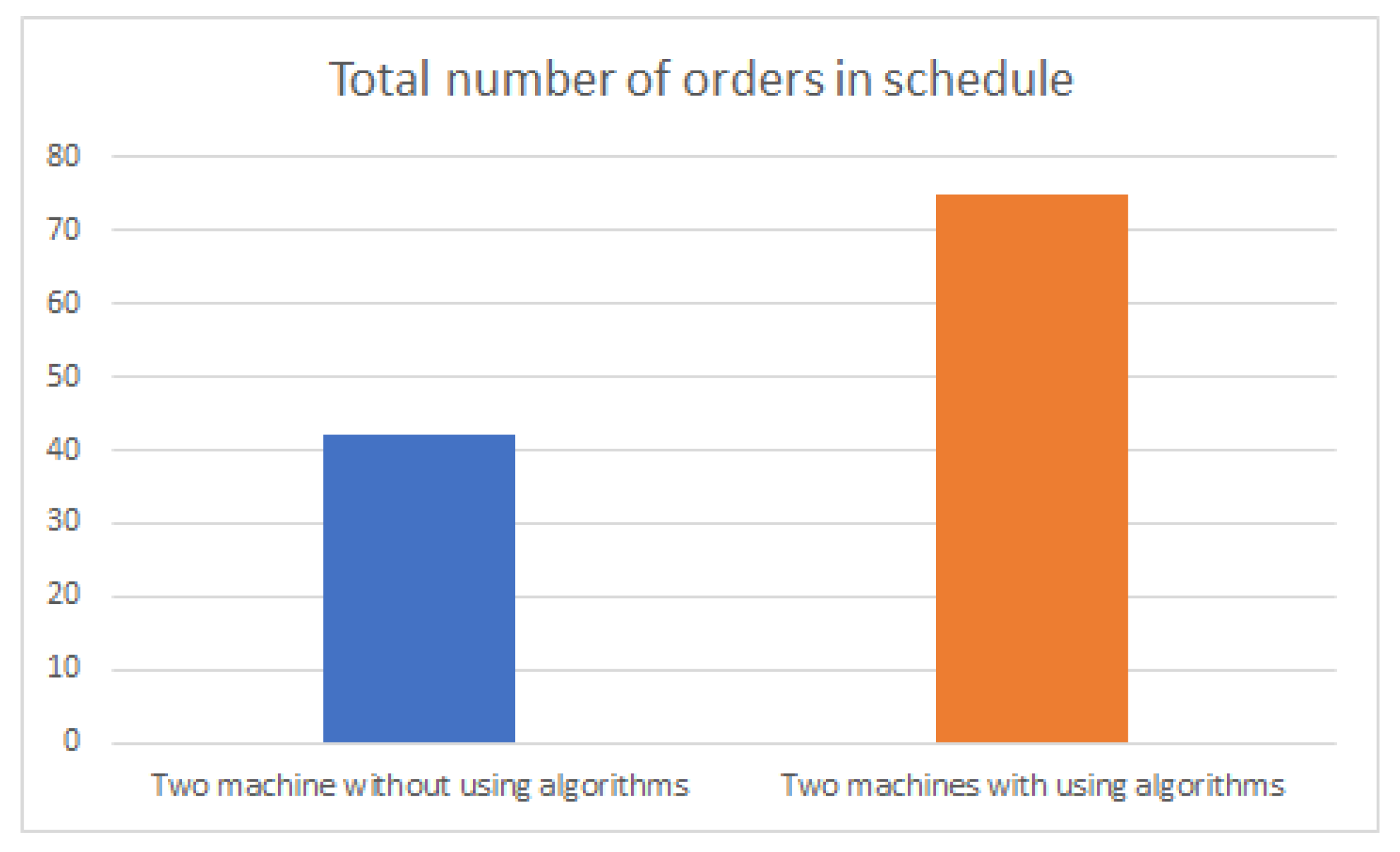
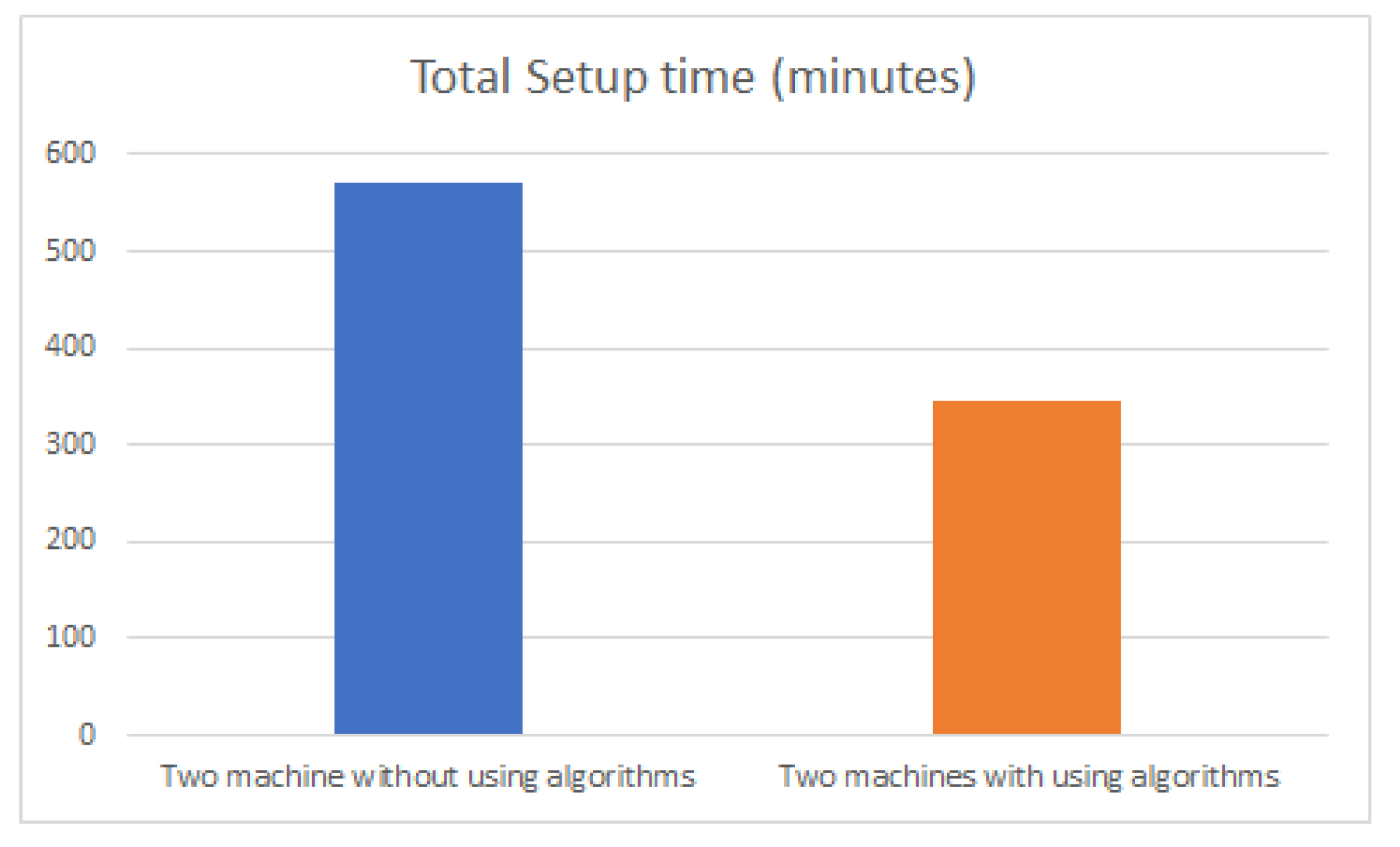
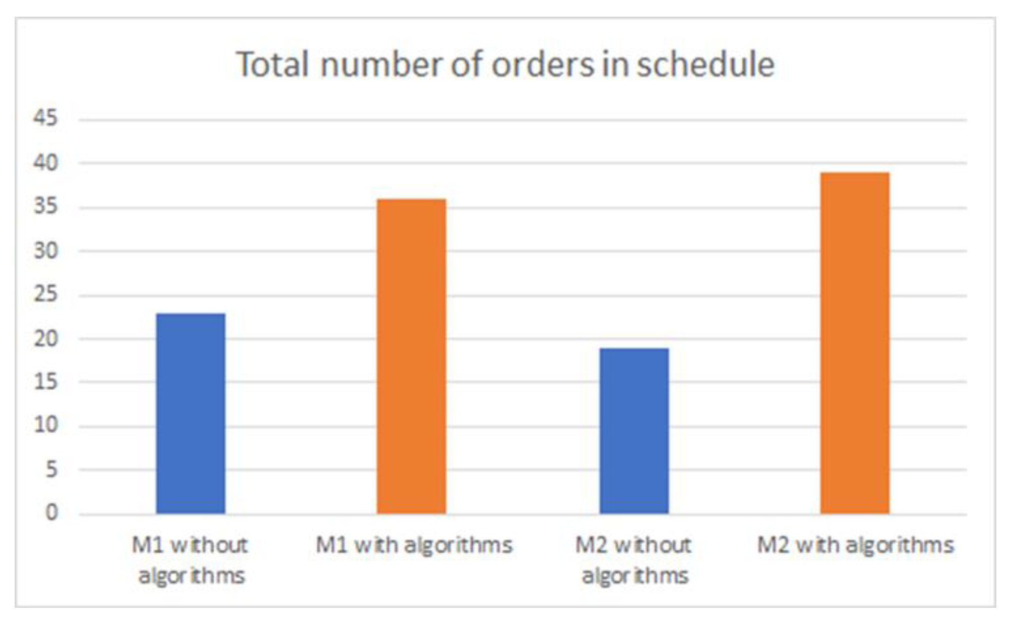
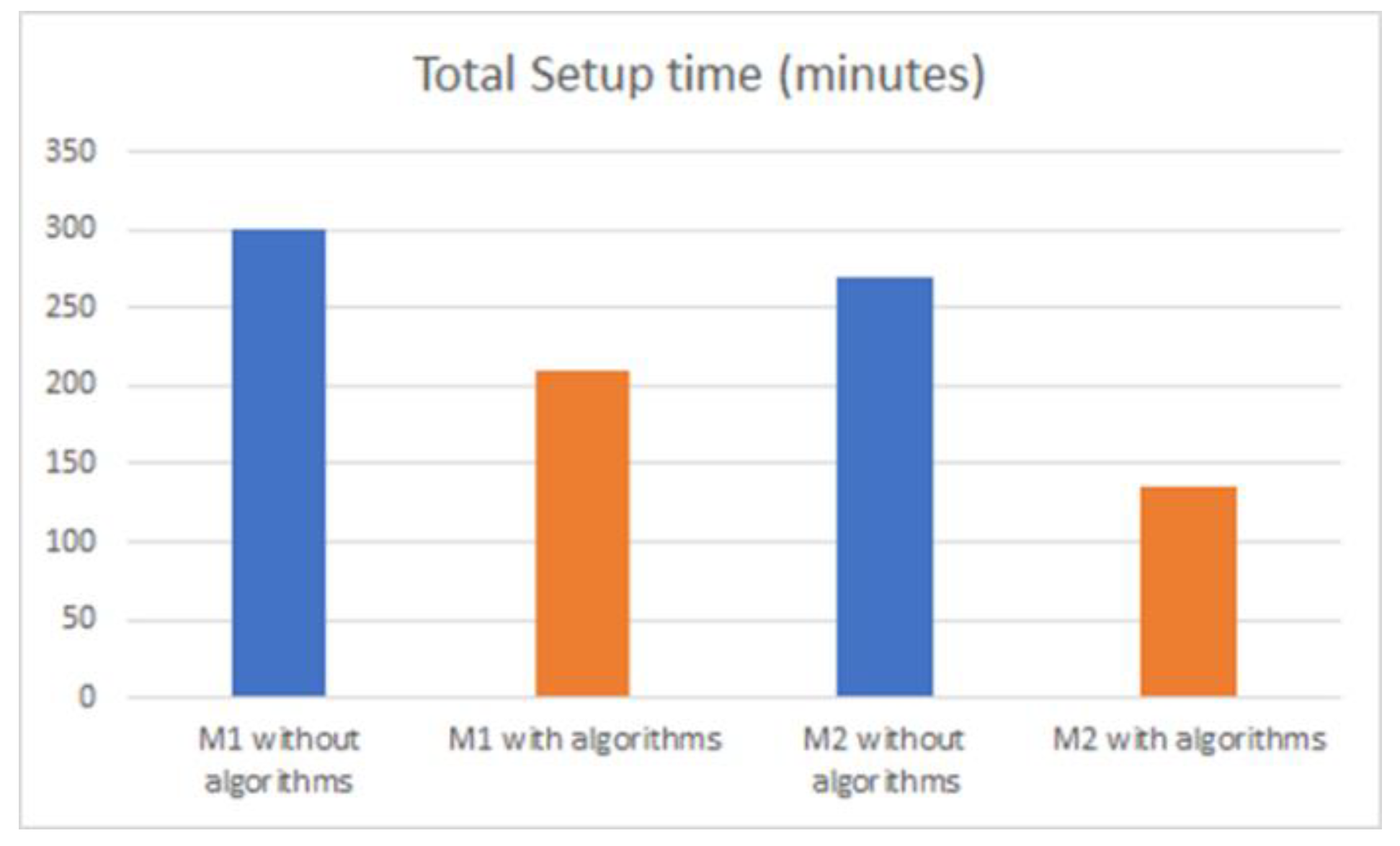
4.2. Result in Two Machines Test

The performances of the total number of orders in the schedule and the total setup time in minutes were evaluated with the use of two machines test, and the results are presented in Figure 8 and Figure 9, respectively. Table 5 shows the overall performance of the total number of orders in the schedule and the total setup time used in the schedule.
Figure 8 shows the overall performance of the total number of orders in the schedule. Before the two machines applied the proposed algorithms, the number of orders arranged in the schedule was 42. The total number of orders in the schedule has increased to 75 after applying the proposed algorithms. There were 33 orders increased after applying the proposed algorithms.
Figure 9 presents the overall performance of the setup time for two machines. The total amount of setup time before these two machines applied the proposed algorithms used about 570 min, which was 9 h and 30 min to change material. Given this, most of the time in the production line was used to change material. Hence, the material changing lead time was very high. However, the total time for the setup of two machines was decreased to 345 min which was 5 h 45 min, while the overall setup time was reduced by approximately 40% after applying the proposed algorithms. Table 6 shows the total number of orders in the schedule and the total setup time used in the schedule for each machine during the two machines’ test.
Figure 10 shows the changes of the two machines with and without applying the proposed algorithm. For the first machine, M1, the schedule generates 23 orders without applying the algorithms, and it reached 36 orders after applying the proposed algorithm. For the second machine, M2, at first, it only got 19 orders. Once the proposed algorithms were applied, the number of orders reached 39 in the schedule.
Figure 11 shows the performance of the total setup times for each machine. When the proposed algorithm was not applied to machine M1, the total setup time for M1 is 300 min. It was the same as machine 2, which had a total of 270 min for setup time. When the proposed algorithm was applied to these two machines, the setup time for machine M1 was reduced to 210 min and reduced to 135 min for M2. This is expected due to the fact that the factor of setup time imposed additional constraints on the scheduling problem. The reduced setup times had minimized the idle time of the machines and created more balanced schedules.

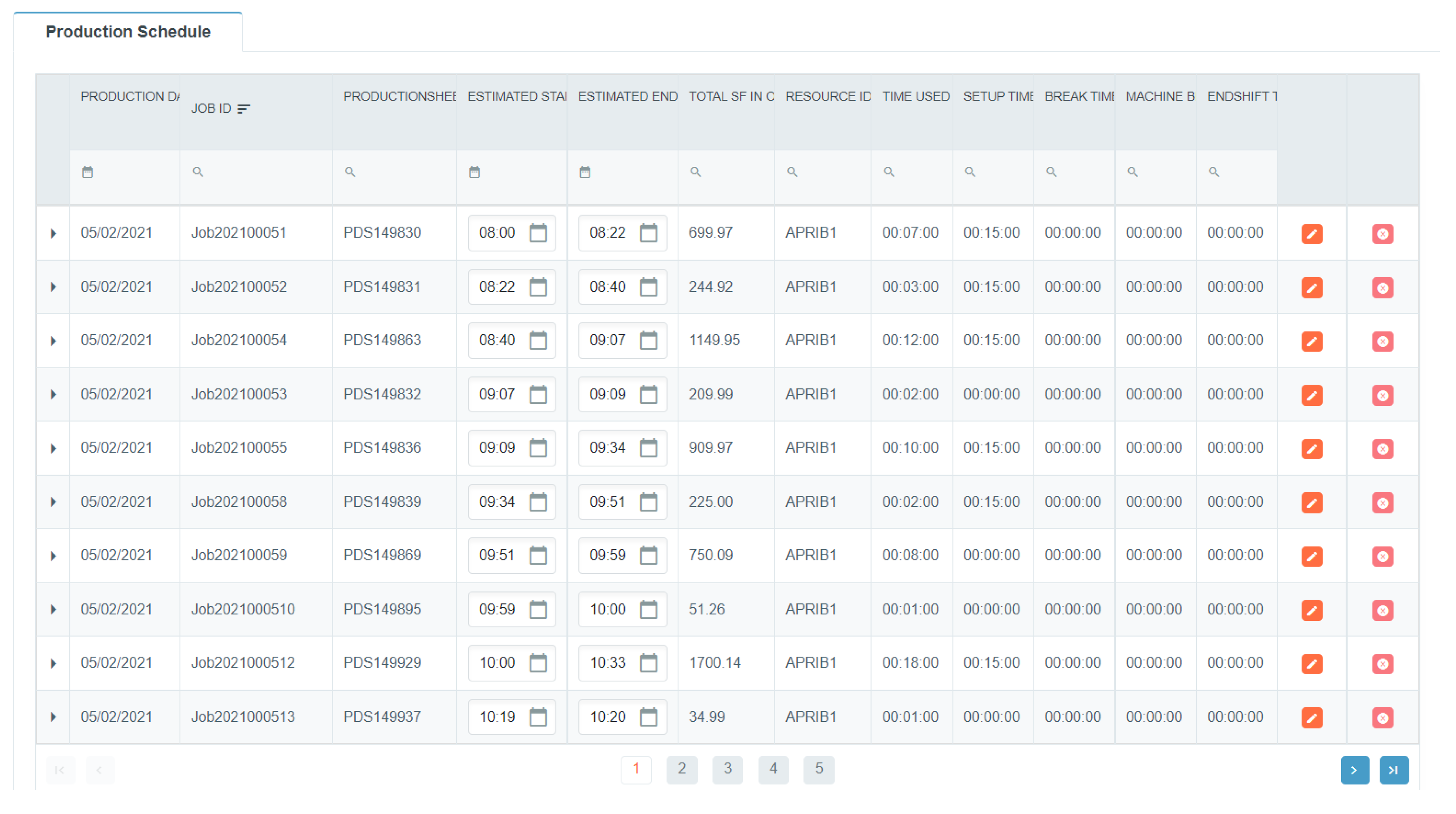
4.3. Information Provided through User Interface

After Algorithms A1 and A2 were implemented, the system generated the production schedule, as shown in Figure 12. Subsequently, the planner had to confirm the schedule based on the domain experience and the standard operating procedure of the company. This is in conjunction with the limitation discovered in the previous study [17], where the methodology to implement a smart production planning and control requires experience and judgement to guarantee that all the relevant contextual variables have been taken into account when evaluating the fit of objectives and priorities with the planning environment variables.
Figure 12 shows the schedule information, such as production date, JobID, production ID, estimated start time, estimated end time, total in square feet per order, resource ID, time used, setup time, break time, machine break time, and end shift time. Each JobID consists of one or more order items. According to the information shown in the system, users can easily understand the arrangement of the orders, the estimated start time and end time, the total square feet used per order, the machines assigned, the time to produce the order, the setup time, break time, and break down time. This has allowed the planners to have a general view of the production schedule and made it easier for them to perform adjustments. In terms of the computational time, it took from 4 to 6 s for one machine process and from 7 to 9 s for two machines to process. However, the computational time might be affected by the existing network infrastructure.

5. Conclusions

In this work, we applied dispatch rule algorithms to the problem of production planning in a roofing manufacturing industry. With the priority level set by the proposed dispatch rule, the optimal sequence of orders was achieved. Besides that, the proposed algorithm was also able to cater for the ever-changing demand of customers in the roof manufacturing industry. We demonstrated that the sorting optimization was achieved by maximizing the total number of orders produced in a day of working hours. Besides that, the algorithm that grouped materials into the same color and thickness successfully reduced the material changing lead time. The results show that the proposed algorithms successfully reduced 47.3% and 40% of the material changing lead time in the first test and the second test, respectively. Besides that, our work balanced the production line through the use of dispatch rules by increasing the number of setup activities performed by both machines. It also helped to reduce the duration of the whole production process, as shown in Figure 1. Currently, the proposed method focuses only on one product. In future work, it will be important to examine the rules on a per-product basis and investigate alternative strategies for more dynamic planning.

Author Contributions

Conceptualization, Y.M.L.; Data curation, S.C.X.R.; Formal analysis, S.C.X.R.; Funding acquisition, W.P.L. and T.T.T.; Investigation, S.C.X.R.; Methodology, S.C.X.R.; Project administration, Y.M.L. and W.P.L.; Resources, S.C.X.R., Y.M.L. and W.P.L.; Software, S.C.X.R.; Supervision, J.K.C.; Writing—original draft, S.C.X.R.; Writing—review & editing, J.K.C. and C.W.F. All authors have read and agreed to the published version of the manuscript.

Funding

This research was funded by Asia Roofing Sdn. Bhd. grant number 77008 and the APC was funded by Inti International University.

Institutional Review Board Statement

Not applicable.

Informed Consent Statement

Not applicable.

Data Availability Statement

The data that support the findings of this study are not publicly available due to privacy or ethical and commercial restrictions.

Acknowledgments

The research work presented in this paper is supported by Asia Roofing Industries Sdn. Bhd. In addition, the authors also would like to thank Fast Track SBOi Sdn. Bhd. for supporting the system interoperability.

Conflicts of Interest

The authors declare no conflict of interest.

Appendix A

Figure A1. Scheduling algorithm flow chart.
Applsci 12 06499 g0a1

Appendix B

Algorithm A1 Arrange Orders with Priority Level (di + Ci,j-1 + Pij)
1Begin
2 /* select order with delivery date */
3 Input Df
4 /* Arrange order by First In First Out and Priority */
5 Ao = order arranged according to priority level (color, thickness, product and
6 Length (desc))
7 /* Grouping according to same product number*/
8 Go = Group orders according to the production number
9END

Appendix C

Algorithm A2 Assign Order to Machine Using SPT and Balancing (Balancing + Pij)
1Begin
2 /* get machine available time */
3 Get MAT
4 /* get Grouped Order */
5 Get Go
6 /* balancing with more than one machine*/
7 FOR each o in Go
8 Create Job in schedule
9 /* get the machine that has more available time */
10 Get M = MAT > = Pi
11 /* check with previous color and thickness */
12 IF Coc == Poc && Cot == Pot THEN
13 Do not Add STi
14 Assign to previous M
15 ELSE
16 Add STi
17 Get M = MAT > = Pi
18 END IF
19 END LOOP
20END

References

  1. Teh, S.; Kee, D. The readiness of small and medium enterprises for the industrial revolution 4.0. GATR Glob. J. Bus. Soc. Sci. Rev. 2019, 7, 217–223. [Google Scholar] [CrossRef]
  2. Malaysian Investment Development Authority. Supporting SMEs in the Adoption of Industry 4.0—Industry4WRDIntervention Fund. 2021. Available online: https://www.mida.gov.my/home/supporting-smes-in-the-adoption-of-industry-4.0---industry4wrd-intervention-fund (accessed on 30 October 2021).
  3. Raj, P.; Wahab, S.; Mohd Zawawi, N.; Awang, K.; Adeeba Wan Ibrahim, W. The benefits of Industry 4.0 on Sustainable Development and Malaysia’s Vision. IOP Conf. Ser. Earth Environ. Sci. 2020, 549, 012080. [Google Scholar] [CrossRef]
  4. Jabri, A.; El Abbassi, I.; Darcherif, A.; El Barkany, A.; Hassani, Z. Planning and scheduling problems of production systems: Review, classification and opportunities. Int. J. Product. Qual. Manag. 2019, 28, 372. [Google Scholar] [CrossRef] [Green Version]
  5. Horváth, D.; Szabó, R. Driving forces and barriers of Industry 4.0: Do multinational and small and medium-sized companies have equal opportunities? Technol. Forecast. Soc. Change 2019, 146, 119–132. [Google Scholar] [CrossRef]
  6. Cotrino, A.; Sebastián, M.; González-Gaya, C. Industry 4.0 HUB: A Collaborative Knowledge Transfer Platform for Small and Medium-Sized Enterprises. Appl. Sci. 2021, 11, 5548. [Google Scholar] [CrossRef]
  7. Szafranek, M.; Michalski, R.; Wiechetek, L. Information Systems for Supporting Production Processes in a Company Manufacturing Roof Metal Sheets—A Case Study. In Proceedings of the Management, Knowledge and Learning Joint International Conferenc, Timisoara, Romania, 25–27 May 2016. [Google Scholar]
  8. Alvarez, E. Multi-plant production scheduling in SMEs. Robot. Comput.-Integr. Manuf. 2007, 23, 608–613. [Google Scholar] [CrossRef]
  9. Gelders, L.; Van Wassenhove, L. Production planning: A review. Eur. J. Oper. Res. 1981, 7, 101–110. [Google Scholar] [CrossRef]
  10. Xu, W.; Zhang, Q.; Ma, J. Effect of customer demand and competitive strategy on decision-making of manufacturing system functional objectives. J. Ind. Eng. Manag. 2013, 6, 1238–1254. [Google Scholar] [CrossRef] [Green Version]
  11. Swaminathan, G. The pros & cons of business innovation at IT organizations. Shanlax Int. J. Manag. 2019, 7, 82–85. [Google Scholar]
  12. Chan, W.; Hu, H. Production scheduling for precast plants using a flow shop sequencing model. J. Comput. Civ. Eng. 2002, 16, 165–174. [Google Scholar] [CrossRef]
  13. Sunday, A.; Omolayo, M.; Samuel, A.; Samuel, O.; Abdulkareem, A.; Moses, E.; Olamma, U. The role of production planning in enhancing an efficient manufacturing system—An Overview. E3S Web Conf. 2021, 309, 01002. [Google Scholar] [CrossRef]
  14. Sobaszek, Ł.; Świć, A. Scheduling the Process of Robot Welding of Thin-Walled Steel Sheet Structures under Constraint. Appl. Sci. 2021, 11, 5683. [Google Scholar] [CrossRef]
  15. Yağmur, E.; Kesen, S. Integrated production and outbound distribution scheduling problem with due dates. In Developments of Artificial Intelligence Technologies in Computation and Robotics; World Scientific: Singapore, 2020. [Google Scholar]
  16. Georgiadis, G.; Elekidis, A.; Georgiadis, M. Optimization-Based Scheduling for the Process Industries: From Theory to Real-Life Industrial Applications. Processes 2019, 7, 438. [Google Scholar] [CrossRef] [Green Version]
  17. Oluyisola, O.E.; Bhalla, S.; Sgarbossa, F.; Strandhagen, J.O. Designing and developing smart production planning and control systems in the industry 4.0 era: A methodology and case study. J. Intell. Manuf. 2022, 33, 311–332. [Google Scholar] [CrossRef]
  18. Khin, A.; Chiun, F.; Seong, L. Identifying the factors of the successful implementation of belt and road initiative on small–medium enterprises in malaysia. China Rep. 2019, 55, 345–363. [Google Scholar] [CrossRef]
  19. SME Definition. Available online: https://smecorp.gov.my/index.php/en/policies/2020-02-11-08-01-24/sme-definition?id=371 (accessed on 2 May 2022).
  20. Zhang, J.; Ding, G.; Zou, Y.; Qin, S.; Fu, J. Review of job shop scheduling research and its new perspectives under Industry 4.0. J. Intell. Manuf. 2017, 30, 1809–1830. [Google Scholar] [CrossRef]
  21. Mohan, J.; Lanka, K.; Rao, A. A review of dynamic job shop scheduling techniques. Procedia Manuf. 2019, 30, 34–39. [Google Scholar] [CrossRef]
  22. Xu, R.; Chen, H.; Liang, X.; Wang, H. Priority-based constructive algorithms for scheduling agile earth observation satellites with total priority maximization. Expert Syst. Appl. 2016, 51, 195–206. [Google Scholar] [CrossRef]
  23. Leusin, M.; Frazzon, E.; Uriona Maldonado, M.; Kück, M.; Freitag, M. Solving the Job-Shop Scheduling Problem in the Industry 4.0 Era. Technologies 2018, 6, 107. [Google Scholar] [CrossRef] [Green Version]
  24. Fazel Zarandi, M.; Sadat Asl, A.; Sotudian, S.; Castillo, O. A state of the art review of intelligent scheduling. Artif. Intell. Rev. 2018, 53, 501–593. [Google Scholar] [CrossRef]
  25. Ospina, G.; De Landtsheer, R. Towards distributed local search through neighborhood combinators. In Proceedings of the 10th International Conference on Operations Research and Enterprise Systems, Vienna, Austria, 4–6 February 2021. [Google Scholar]
  26. Desale, S.; Rasool, A.; Andhale, S.; Rane, P. Heuristic and meta-heuristic algorithms and their relevance to the real world: A Survey. Int. J. Comput. Eng. Res. Trends 2015, 351, 2349–7084. [Google Scholar]
  27. Ding, J.; Song, S.; Gupta, J.; Zhang, R.; Chiong, R.; Wu, C. An improved iterated greedy algorithm with a tabu-based reconstruction strategy for the no-wait flowshop scheduling problem. Appl. Soft Comput. 2015, 30, 604–613. [Google Scholar] [CrossRef]
  28. Chiang, T.; Che, Z.; Lee, C.; Liang, W. Applying Clustering Methods to Develop an Optimal Storage Location Planning-Based Consolidated Picking Methodology for Driving the Smart Manufacturing of Wireless Modules. Appl. Sci. 2021, 11, 9895. [Google Scholar] [CrossRef]
  29. Ðurasević, M.; Jakobović, D. A survey of dispatching rules for the dynamic unrelated machines environment. Expert Syst. Appl. 2018, 113, 555–569. [Google Scholar] [CrossRef]
  30. Zhang, F.; Mei, Y.; Zhang, M. Evolving Dispatching Rules for Multi-objective Dynamic Flexible Job Shop Scheduling via Genetic Programming Hyper-heuristics. In Proceedings of the 2019 IEEE Congress on Evolutionary Computation (CEC), Wellington, NZ, USA, 10–13 June 2019. [Google Scholar]
  31. Hung, Y.; Chen, I. A simulation study of dispatch rules for reducing flow times in semiconductor wafer fabrication. Prod. Plan. Control. 1998, 9, 714–722. [Google Scholar] [CrossRef]
  32. Zhang, H.; Roy, U. A semantics-based dispatching rule selection approach for job shop scheduling. J. Intell. Manuf. 2018, 30, 2759–2779. [Google Scholar] [CrossRef]
  33. Xiong, H.; Fan, H.; Jiang, G.; Li, G. A simulation-based study of dispatching rules in a dynamic job shop scheduling problem with batch release and extended technical precedence constraints. Eur. J. Oper. Res. 2017, 257, 13–24. [Google Scholar] [CrossRef]
  34. Mittler, M.; Schoemig, A. Comparison of dispatching rules for reducing the mean and variability of cycle times in semiconductor manufacturing. In Operations Research Proceedings; Springer: Berlin/Heidelberg, Germany, 1999; pp. 479–485. [Google Scholar]
  35. Alfieri, A. Due date quoting and scheduling interaction in production lines. Int. J. Comput. Integr. Manuf. 2007, 20, 579–587. [Google Scholar] [CrossRef]
  36. Zhang, H.; Jiang, Z.; Guo, C. Simulation-based optimization of dispatching rules for semiconductor wafer fabrication system scheduling by the response surface methodology. Int. J. Adv. Manuf. Technol. 2008, 41, 110–121. [Google Scholar] [CrossRef]
  37. Huh, J.; Park, I.; Lim, S.; Paeng, B.; Park, J.; Kim, K. Learning to dispatch operations with intentional delay for re-entrant multiple-chip product assembly lines. Sustainability 2018, 10, 4123. [Google Scholar] [CrossRef] [Green Version]
  38. Vespoli, S.; Grassi, A.; Guizzi, G.; Santillo, L. Evaluating the advantages of a novel decentralised scheduling approach in the Industry 4.0 and Cloud Manufacturing era. IFAC-PapersOnLine 2019, 52, 2170–2176. [Google Scholar] [CrossRef]
  39. Liu, B.; Qiu, S.; Li, M. Simultaneous Scheduling Strategy: A novel method for flexible job shop scheduling problem. In Proceedings of the 2020 IEEE Congress on Evolutionary Computation (CEC), Glasgow, UK, 19 July 2020. [Google Scholar]
  40. Guerreiro, N.; Hagen, G.; Maddalon, J.; Butler, R. Capacity and throughput of urban air mobility vertiports with a first-come, first-served vertiport scheduling algorithm. In Proceedings of the AIAA Aviation 2020 Forum, Online, 15–19 June 2020. [Google Scholar]
  41. Arima, S.; Zhang, Y.; Akiyama, Y.; Ishizaki, Y. Dynamic scheduling of product-mix production systems of MTS and MTO. In Proceedings of the 2017 Joint International Symposium on e-Manufacturing and Design Collaboration (eMDC) & Semiconductor Manufacturing (ISSM), Hsinchu, Taiwan, 15 September 2017. [Google Scholar]
  42. Ma, Z.; Yang, Z.; Liu, S.; Wu, S. Optimized rescheduling of multiple production lines for flowshop production of reinforced precast concrete components. Autom. Constr. 2018, 95, 86–97. [Google Scholar] [CrossRef] [Green Version]
  43. Ojstersek, R.; Brezocnik, M.; Buchmeister, B. Multi-objective optimization of production scheduling with evolutionary computation: A review. Int. J. Ind. Eng. Comput. 2020, 11, 359–376. [Google Scholar] [CrossRef]
  44. Ma, A.; Nassehi, A.; Snider, C. Balancing multiple objectives with anarchic manufacturing. Procedia Manuf. 2019, 38, 1453–1460. [Google Scholar] [CrossRef]
  45. Grosch, B.; Kohne, T.; Weigold, M. Multi-objective hybrid genetic algorithm for energy adaptive production scheduling in job shops. Procedia CIRP 2021, 98, 294–299. [Google Scholar] [CrossRef]
  46. Chawla, V.; Chanda, A.; Angra, S. Sustainable multi-objective scheduling for automatic guided vehicle and flexibthe le manufacturing system by a grey wolf optimization algorithm. Int. J. Data Netw. Sci. 2018, 2, 27–40. [Google Scholar] [CrossRef]
  47. Zhu, H.; Chen, M.; Zhang, Z.; Tang, D. An Adaptive Real-Time Scheduling Method for Flexible Job Shop Scheduling Problem With Combined Processing Constraint. IEEE Access 2019, 7, 125113–125121. [Google Scholar] [CrossRef]
  48. Trappey, A.; Trappey, C.; Hareesh Govindarajan, U.; Chuang, A.; Sun, J. A review of essential standards and patent landscapes for the Internet of Things: A key enabler for Industry 4.0. Adv. Eng. Inform. 2017, 33, 208–229. [Google Scholar] [CrossRef]
Figure 1. The process from customer order to delivery. Adapted with permission from Ref. [7]. Copyright 2016 Łukasz Wiechetek.
Applsci 12 06499 g001
Figure 2. Manual production planning.
Applsci 12 06499 g002
Figure 3. Types of scheduling algorithms. Adapted with permission from Ref. [20]. Copyright 2019 Yisheng Zou.
Applsci 12 06499 g003
Figure 4. General data flow. The detailed algorithm is presented in Figure 5.
Applsci 12 06499 g004
Figure 5. Detailed algorithm.
Applsci 12 06499 g005
Figure 6. The performance of the number of orders for one machine.
Applsci 12 06499 g006
Figure 7. The performance of total setup time for one machine.
Applsci 12 06499 g007
Figure 8. The overall performance of the number of schedules for two machines.
Applsci 12 06499 g008
Figure 9. The overall performance of setup time for two machines.
Applsci 12 06499 g009
Figure 10. The performance of the total number of orders for each machine.
Applsci 12 06499 g010
Figure 11. The performance of the total setup times for each machine.
Applsci 12 06499 g011
Figure 12. Scheduling Information.
Applsci 12 06499 g012
Table 1. Definition of SMEs in Malaysia. Adapted with permission from Ref. [19]. Copyright 2020 SME Corp. Malaysia Secretariat.
CategoryManufacturing Services and Other Sectors
MediumSales Turnover: RM15 mil to RM50 mil
OR
Employees: From 75 to 200 people
Sales Turnover: RM3 mil to RM20 mil
OR
Employees: From 75 to 200 people
SmallSales Turnover: RM300,000 to RM 15 mil
OR
Employees: From 5 to 75 people
Sales Turnover: RM300,000 to RM3 mil
OR
Employees: From 5 to 30 people
MicroSales Turnover: Less than RM300,000
OR
Employees: Less than 5 people
Sales Turnover: Less than RM300,000
OR
Employees: Less than 5 people
Table 2. Formalization for Dispatch Rule Algorithms.
RuleDefinitionDescription
(1) FIFOCi,j−1Jobs are scheduled for work in the same sequence as they arrive at the machine.
(2) SPTPijJobs are scheduled in ascending order of processing times.
(3) EDDdiJobs are scheduled in ascending order of due dates.
Table 3. Description of production-line notation.
NotationDescription
iJob (i, i + 1 ∈ I)
ITotal of jobs
kMachines (kM)
MThe total number of machines
oOrder (o,o + 1 ∈ PO)
POTotal production orders
AmiThe set of alternative machines on which job i can be processed (AMiM)
OitcDemand of job that cannot be produced on time in day tc
TiSet of total items in the orders
AoArranged orders
GoGrouped orders
McMachine capacity
CocCurrent order color
CotCurrent order thickness
PocPrevious order color
PotPrevious order thickness
STiSetup time of job i
Table 4. The overall performance of the total number of orders and total setup time used in the schedule.
Type of MachineNumber of Orders in ScheduleTotal Setup Time (min)
one machine with using algorithms37150
one machine without using algorithms20285
Table 5. The overall performance of the total number of orders and total setup time used in the schedule.
Total Number of Orders in ScheduleTotal Setup Time (min)
Two machines without using algorithms42570
Two machines using algorithms75345
Table 6. The performance of schedule for each machine in the two machines’ test.
MachinesTotal Number of Orders in ScheduleTotal Setup Time (min)
M1 without algorithms23300
M1 with algorithms36210
M2 without algorithms19270
M2 with algorithms39135
Publisher’s Note: MDPI stays neutral with regard to jurisdictional claims in published maps and institutional affiliations.

