Derivation of a Universally Valid Array Factor of a Conformal Arrays Based on Phase Compensation and Genetic Learning Particle Swarm Optimization

Abstract

In this study, we investigated the recent deterioration of the radiation pattern performance of conformal arrays, which are applied to fields such as aircraft and vehicles. We analyzed the radiation pattern of conformal arrays in the array factor stage by combining previous studies on various beam-forming techniques for conformal arrays. To efficiently calculate and utilize the radiation pattern of conformal arrays, we derived an array factor based on phase composition for nonplanar arrays of three-dimensional (3D) coordinate systems. As an amplitude tapering method for controlling the sidelobe level of the derived 3D array factor, we propose a Bernstein polynomial generalization method based on Genetic Learning Particle Swarm Optimization. The proposed 3D array factor was verified using a cavity-backed patch antenna operating at the X-band through EM simulation of conformal arrays as a single element.

1. Introduction

Recently, there has been an increasing need for the development of conformal arrays used in Unmanned Aerial Vehicles (UAVs) and vehicle platforms. When the conformal arrays are arranged on a curved platform shape, unlike planar arrays that require additional space for arrangement, the resistance to air can be reduced during movement, and RCS can be reduced by decreasing the protruding structure [1]. However, the electrical properties of conformal arrays change according to the curvature of the platform they are applied to, and when an array is curved, such as the noncollinear element arrangements in many common systems [2]. In some systems, nonlinearity occurs because conformal arrays must consider electrical properties in 3D space, unlike planar arrays located on the same plane.

Several studies have been conducted on the phase calculation of the array factor to improve the electrical characteristics of the conformal arrays. The common array phase compensation of the vertical surface situation has been employed [3]. This study confirmed the S-parameter and radiation pattern by applying a 4$\times$4 array to spherical platforms. A common array wide-angle scanning method has also been reported for vertical surface situations [4]. The authors performed beam scanning of up to 50${}^{\circ }$ on conformal arrays. To improve the phase of the conformal arrays, the array factor was not calculated based on the location of the element, but the location was expressed as a location on the platform, considering the shape of the platform. However, each time the shape of the platform changes, the calculation formula must be changed (the equation for location calculation according to the shape of the platform appears differently every time).

Herein, we propose a unified phase calculation method employing coordinates in three-dimensional (3D) space based on the phase composition method for common arrays that include all the previous studies. Unlike previous studies that focused on specific platforms, this method applies to all random array grids and nonlinear arrays. Depending on the characteristics of a conformal array, beamforming through amplitude control is difficult. This differs from the case of widely used planar arrays based on the non-periodicity and additional coordinate axes. Amplitude tapering of conformal arrays has also been studied. Based on the elevation beam design method for airborne conformal arrays, the amplitude optimization has been studied for only one situation by optimizing the Bernstein polynomial [5]. In beam synthesis for conformal-array antennas with efficient tapering, the amplitude has been applied using the Least Square Method [6]. Conformal-array amplitude weight optimization has also been employed using the Bezier curve [7]. In addition, aperiodic and conformal arrays have been studied [8,9,10,11,12,13,14,15,16]. Previous studies on the amplitude application method for conformal arrays have shown aspects that do not consider phase-related parts and those that are applicable to only one case. We propose an amplitude tapering method that optimizes the above-described phase calculation method and Bernstein polynomials through Genetic Learning Particle Swarm Optimization (GLPSO) [17]. The performance of the proposed method is improved based on the array factor of conformal arrays, which is confirmed by CST simulations and MATLAB.

The rest of the paper is arranged as follows. Pattern degradation improvement of conformal arrays and the array factor for nonplanar arrays are derived in Section 2.1 through phase compensation and verified in Section 2.2 by comparing the EM simulation and array factor calculations based on the derived array factor. In Section 2.3, we propose an amplitude tapering method to which the derived array factor could be applied. In Section 3, we verify the final array factor to which the proposed phase calculation and the amplitude tapering methods are applicable. Conclusions are presented in Section 4.

2. Derivation of 3D Array Factor

2.1. Improvement of Pattern Degradation of Conformal Arrays through Phase Compensation

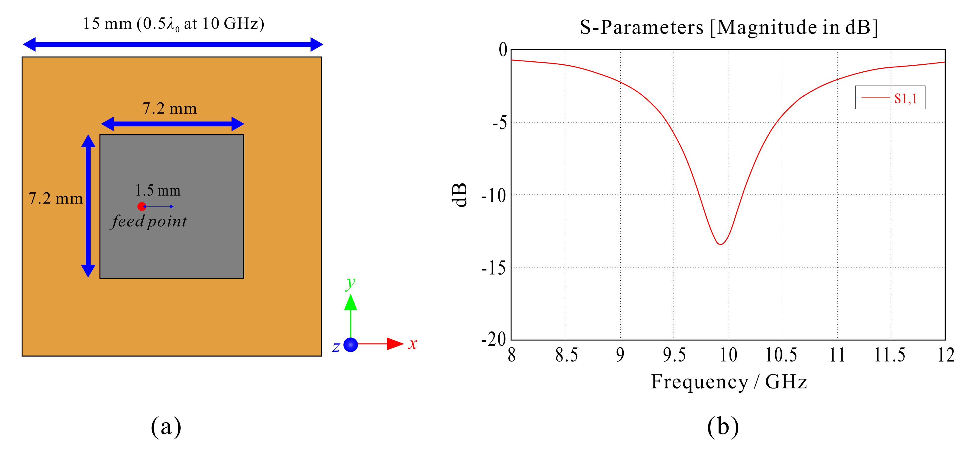
To investigate the change in electrical characteristics according to the platform shape of the conformal arrays, we designed a patch antenna operating at 10 GHz (Figure 1). Taconic’s RF-35 (dielectric constant = 3.5) was used as a substrate for the patch antenna with a thickness of 1.52 mm. Coaxial feeding was employed, and the broadside gain of a single radiation element was about 6.2 dB. In the patch antenna, the radiating element has the size of x-direction element spacing, dx = 0.5$\lambda$, and y-direction element spacing, dy = 0.5$\lambda$ (15 mm). We compared the pattern performance of a 12$\times$24 planar array using the designed patch antenna as a single radiation element and the radiation pattern of a 12$\times$24 conformal array.

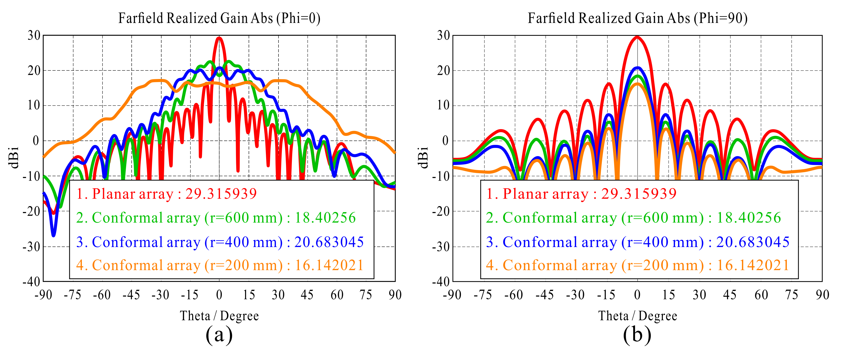
The conformal array is cylindrical, and the variable r is the radius of the cylindrical array platform, as shown in Figure 2. When r for the 12$\times$24 planar and the conformal arrays is r = 200, 400, and 600 mm, the 2D radiation patterns under uniform amplitude and in-phase feeding are as shown in Figure 3.

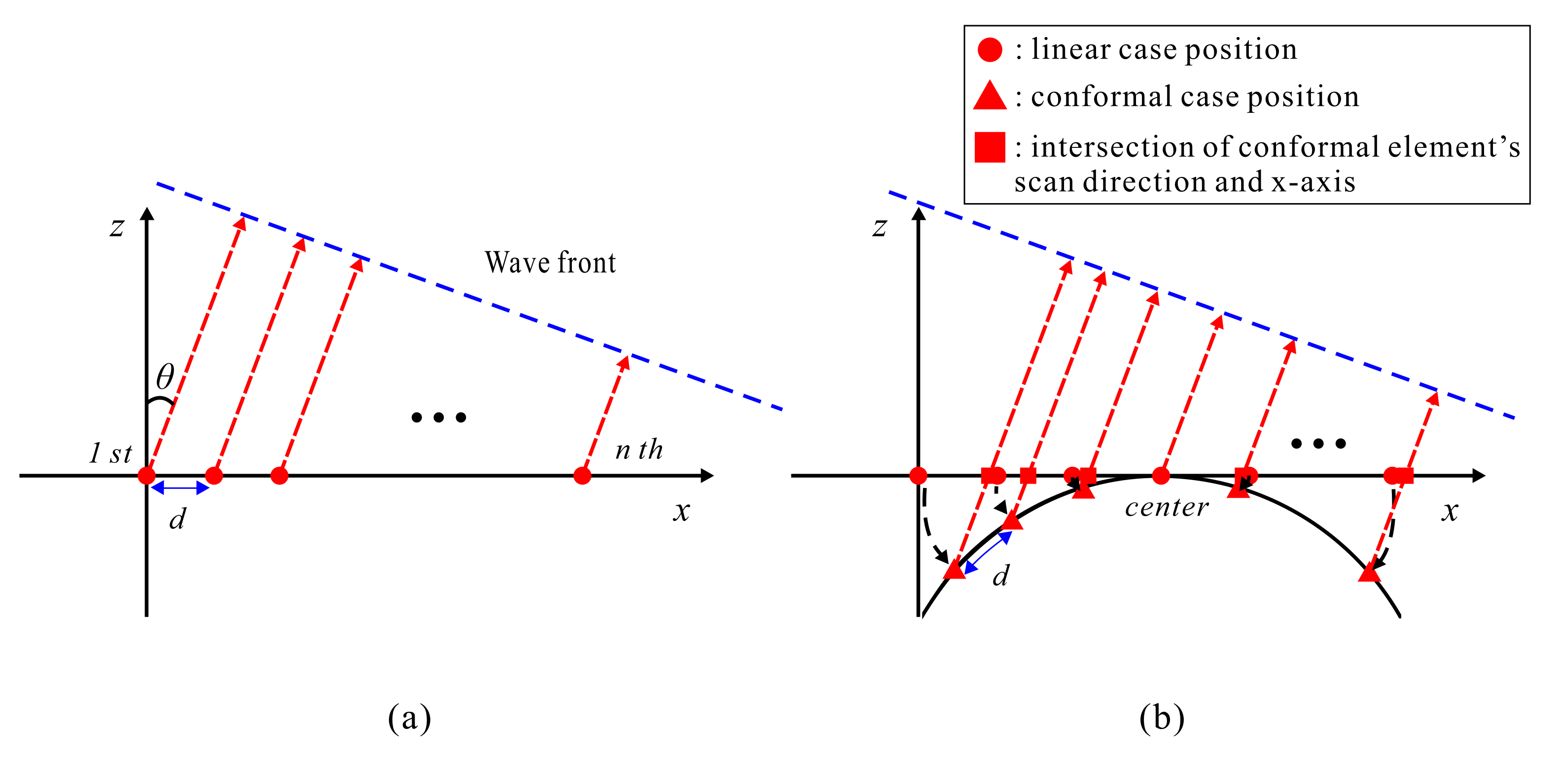
The pattern of the conformal array significantly differs from that of the planar array according to the change in the platform (change in r) even with the same radiating element shape, number of radiating elements, and radiating element spacing. In the presented case, as r becomes shorter (as the curvature increases), the element location situation changes, and it can be seen that the gain is decreased and the beam is widely distributed due to the phase difference up to the same-phase wave front. The cause of performance degradation in uniform feeding was analyzed from a phase perspective by schematically illustrating a cylindrical situation bent along the x-axis.

Figure 4a shows the position of each radiation element in a planar array condition. Unlike the planar array (Figure 4a), the z-axis coordinates for the conformal array changes for each radiation element as the element position changes over the curve (Figure 4b). To obtain the phase length to the wavefront in Figure 4b, the array factor of the conformal array can be calculated by considering the z-axis coordinates or the phase compensation for the phase delay, which is the distance from the actual element position to the x-axis. In other words, for uniform amplitude feeding, conformal arrays require the modification of the array factor (Equation (1)) used for planar arrays.

$${\displaystyle A{F}_{planar}=\sum _{k=1}^{M·N}{e}^{j[(\frac{2\pi }{\lambda }{x}_{k}sin\left(\theta \right)cos\left(\varphi \right)+\frac{2\pi }{\lambda }{y}_{k}sin\left(\theta \right)sin\left(\varphi \right))-(\frac{2\pi }{\lambda }{x}_{k}sin\left({\theta }_0\right)cos\left({\varphi }_0\right)+\frac{2\pi }{\lambda }{y}_{k}sin\left({\theta }_0\right)sin\left({\varphi }_0\right))]}}$$

(1)

When the positions of the elements in Figure 4a correspond to the XZ plane, as shown in Figure 4b, it can be represented as shown in Figure 5. The element coordinate of the planar array $P_k$ is moved to that in the form of a conformal array. To calculate the phase on the x-axis, we consider the phase difference as much as $phasedela{y}_k$, which is the length between the corresponding positions $P_k^{{}^{\prime }}$ and $P_k^{{}^{\prime \prime }}$ on the x-axis. If Equation (1) is solved considering the phase difference of $phasedela{y}_k$ for the conformal array, the array factor in Figure 4b can be obtained. The phase difference $phasedela{y}_k$ can be expressed as follows.

$$phasedela{y}_k=\frac{|z_k|}{cos\left({\theta }_0\right)}$$

(2)

Assuming that the interval between elements of conformal arrays is 0.5$\lambda$, $P_k^{{}^{\prime }}$, $P_k^{{}^{\prime \prime }}$ is expressed as follows:

$$P_k^{{}^{\prime }}=(x_k,0,z_k)$$

(3)

$$P_k^{{}^{\prime \prime }}=(x_k-z_k·tan\left({\theta }_0\right),0,0)$$

(4)

This is based on the corresponding coordinates $P_k^{{}^{\prime \prime }}$ considering the phase difference, which is substituted into Equation (1) and calculated as follows:

$${\displaystyle A{F}_{example}=\sum _{k=1}^K{e}^{j[\frac{2\pi }{\lambda }(x_k-z_{k}tan\left({\theta }_0\right))sin\left(\theta \right)-\frac{2\pi }{\lambda }(x_k-z_{k}tan\left({\theta }_0\right))sin\left({\theta }_0\right)]}\times e^{-j\frac{2\pi }{\lambda }·phasedela{y}_k}}$$

(5)

Substituting $phasedela{y}_k$ into Equation (5) and rearranging z, we obtain Equation (6).

$${\displaystyle A{F}_{example}=\sum _{k=1}^K{e}^{j[\frac{2\pi }{\lambda }(x_{k}sin\left(\theta \right))-\frac{2\pi }{\lambda }(x_{k}sin\left({\theta }_0\right))]}\times e^{j[\frac{2\pi }{\lambda }(z_{k}cos\left(\theta \right))-\frac{2\pi }{\lambda }(z_{k}cos\left({\theta }_0\right))]}}$$

(6)

As expressed in Equation (6), the array factor considering $phasedela{y}_k$ in the uniform amplitude feeding example for cylindrical conformal arrays is converted into a universal coordinate equation including the z-coordinate. In a case where y-axis coordinates do not exist, the variable for $\varphi$ is excluded because the value of $\varphi$ cannot be adjusted. For 3D expansion, we consider the y-axis coordinates and $\varphi$ in the array factor. Since the coordinates on the z-axis do not change with a change in $\varphi$, it maintains the form (z$cos\left(\theta \right)$), which changes only under the change of $\theta$. The xy plane changes to a shape displayed on the UV plane (x$sin\left(\theta \right)$$cos\left(\varphi \right)$, y$sin\left(\theta \right)$$sin\left(\varphi \right)$).

If this is expanded with respect to point $A_i$ on the 3D coordinate axis of the elements constituting an arbitrary array shape including the y-axis coordinate, $A_i$ is expressed as follows:

$$A_i=(x_i,y_i,z_i),i=1,2,3,\cdots ,I$$

(7)

$$\begin{array}{c}{\displaystyle A{F}_{uniform}=\sum _{i=1}^I{e}^{j[\frac{2\pi }{\lambda }(x_{i}sin\left(\theta \right)cos\left(\varphi \right))-\frac{2\pi }{\lambda }(x_{i}sin\left({\theta }_0\right)cos\left({\varphi }_0\right))]}}\hfill \\ \times e^{j[\frac{2\pi }{\lambda }(y_{i}sin\left(\theta \right)sin\left(\varphi \right))-\frac{2\pi }{\lambda }(y_{i}sin\left({\theta }_0\right)sin\left({\varphi }_0\right))]}\times e^{j[\frac{2\pi }{\lambda }(z_{i}cos\left(\theta \right))-\frac{2\pi }{\lambda }(z_{i}cos\left({\theta }_0\right))]}\hfill \end{array}$$

(8)

We propose an equation that can calculate the phase regardless of the grid format, curvature, and nonlinearity if the positions of all possible elements that can be specified on the 3D coordinate axis are located through the array factor for uniform amplitude feeding in Equation (8).

2.2. Results of Array Factor Calculation through Simulations

We verified the 3D array factor by simulating a situation of uniform amplitude feeding based on the proposed equation for the 3D array factor. In the form of a single element, we designed a cavity-backed patch antenna operating at 10 GHz.

The designed cavity-backed patch antenna is shown in Figure 6a. RF-35 (dielectric constant = 3.5) from Taconic with a thickness of 0.51 mm was used as a substrate for the antenna. The substrate is 15 mm on the x-axis and 15 mm on the y-axis. The cavity is set to metal with a total length of 7 mm in the z-direction. The cavity is 1.5 mm thickness in the x- and y-direction and 2 mm thickness in the z-direction. The inside of the metal is set to air. Coupling feeding was employed [18,19,20]. The cavity-backed patch antenna (Figure 6a) has a patch size of 7 mm on the x-axis and 7 mm on the y-axis, and the thickness of the cavity layer is 7 mm. The bandwidth of reflection coefficient below −10 dB is 9.242–10.81 GHz, as shown in Figure 6b. The element pattern for the cavity-backed patch antenna is shown in Figure 6c. The broadside gain of the single radiation element is approximately 5.479 dBi.

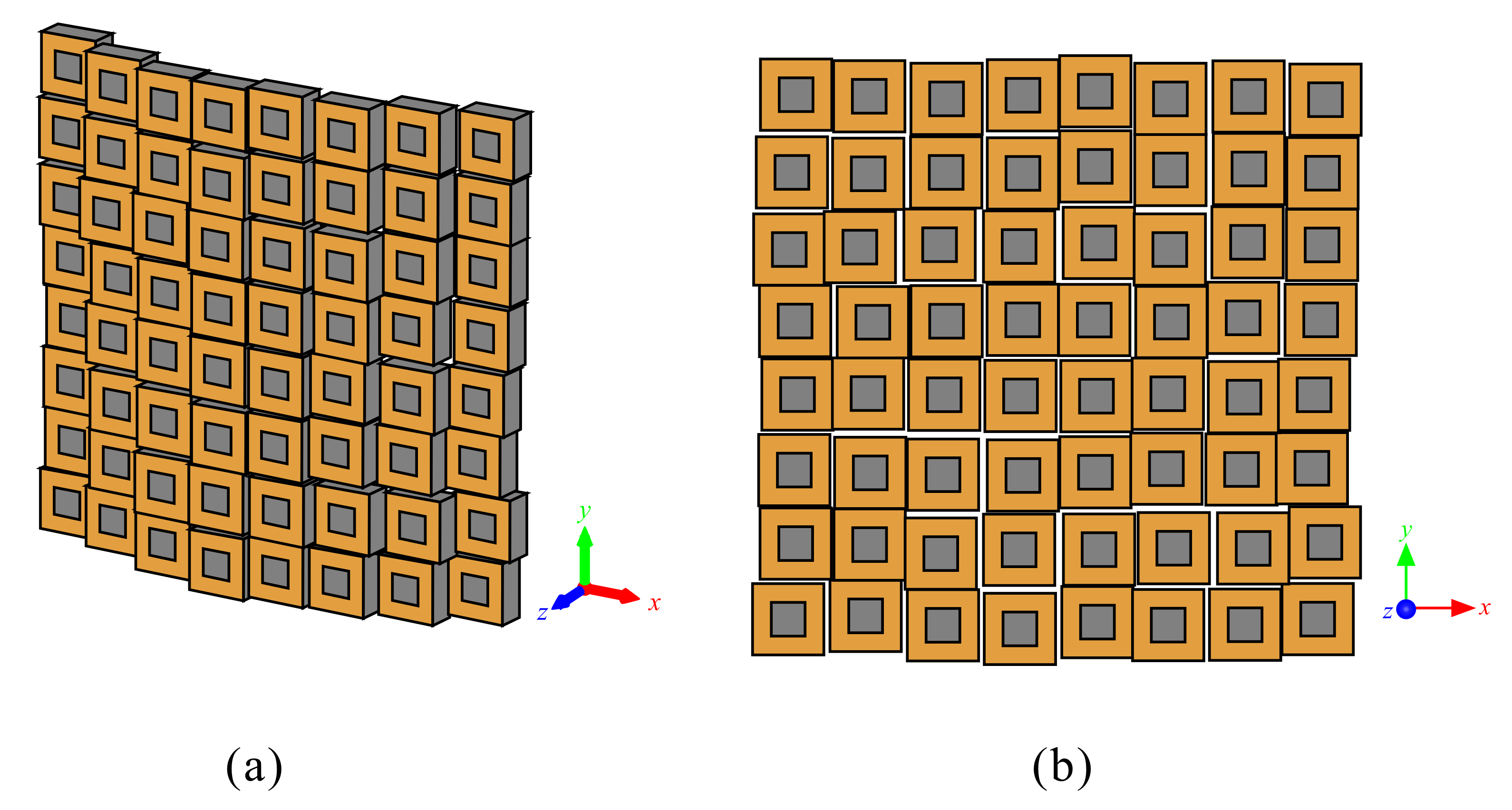
Figure 7 shows the shape of an 8$\times$8 random grid array using the cavity-backed patch antenna as a single radiation element. The element spacing was calculated as the distance between patch centers. The element spacing in the x- and y-directions, dx and dy, respectively, were randomly set to 0.5$\lambda$–0.56$\lambda$ (15–16.8 mm), and that in the z-direction dz was set to 0–0.2$\lambda$ (0–6 mm). The calculated array factor scanned at $\varphi$ = 0${}^{\circ }$, $\theta$ = 30${}^{\circ }$ under uniform amplitude feeding was compared with the radiation pattern obtained from EM simulations.

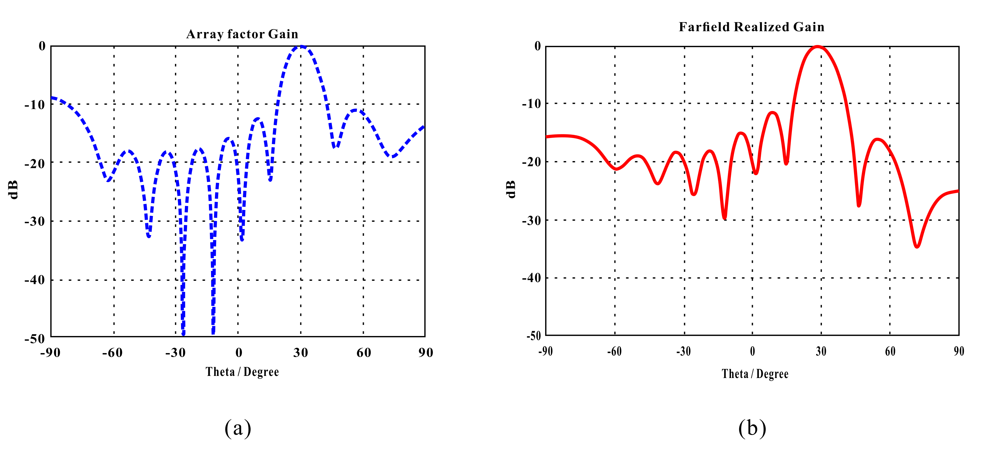
Figure 8 shows the array factor and radiation pattern at 10 GHz when the shape of the conformal array is as shown in Figure 7. Figure 8a shows the 3D array factor calculated using MATLAB, and Figure 8b shows the radiation pattern of the conformal array simulated by substituting the phase obtained from Equation (11). The patterns shown in Figure 8a,b are very similar. However, Figure 8a shows only the calculated array factor, and Figure 8b show the array factor in Figure 8a and the element pattern in Figure 6c, so that the reduction is reflected in the gain of $\theta$ = −90${}^{\circ }$ and $\theta$ = 90${}^{\circ }$.

These confirm that performance prediction and control in the case of 3D and random arrangement can be achieved using the proposed 3D array factor for uniform amplitude feeding (Equation (11)) by calculating an array factor for an arbitrary array and adjusting the element pattern to adjust the array pattern.

2.3. Amplitude Tapering Method of Array Factor (Bernstein Polynomial Using GLPSO)

We confirmed in the preceding subsections that a phase can be calculated for arbitrary arrays that can specify the element position in the 3D coordinate system using the 3D array factor in cases of the uniform amplitude feeding. However, as with planar arrays, it is necessary to adjust the amplitude for the desired side-lobe level (SLL) in conformal arrays. Thus, Equation (10) considering the amplitude $w_i$ of the ith element with respect to the previously proposed $A{F}_{uniform}$ expresses the array factor for the final 3D array.

$$0\le w_i\le 1,i=1,2,3,\cdots ,I$$

(9)

$$\begin{array}{c}{\displaystyle A{F}_{3D}=\sum _{i=1}^I{w}_i\times e^{j[\frac{2\pi }{\lambda }(x_{i}sin\left(\theta \right)cos\left(\varphi \right))-\frac{2\pi }{\lambda }(x_{i}sin\left({\theta }_0\right)cos\left({\varphi }_0\right))]}}\hfill \\ \times e^{j[\frac{2\pi }{\lambda }(y_{i}sin\left(\theta \right)sin\left(\varphi \right))-\frac{2\pi }{\lambda }(y_{i}sin\left({\theta }_0\right)sin\left({\varphi }_0\right))]}\times e^{j[\frac{2\pi }{\lambda }(z_{i}cos\left(\theta \right))-\frac{2\pi }{\lambda }(z_{i}cos\left({\theta }_0\right))]}\hfill \end{array}$$

(10)

However, as with a phase, the conformal array cannot achieve the desired performance using only the amplitude method for planar arrays due to the structural differences and nonlinearity. Consequently, several amplitude tapering methods have been studied for applications in conformal arrays. Conformal-array amplitude tapering has been performed using the Particle Swarm Optimization (PSO) method on Bernstein polynomials based on the structure for conformal array situations, and only amplitude was optimized to increase radiation efficiency and lower SLL [2]. However, it can be used universally because phase-related parts are excluded. It can also be used for a particular case. Herein, based on phase compensation, we employed GLPSO, which is more advanced than PSO, GLSPO combines Genetic Algorithm (GA) and PSO, and whenever an iteration is performed, the entire cluster moves in the optimization direction and causes specific objects to mutate and converge to the global optimum at a high speed [17]. The GLPSO setting was performed using 2000 particles, probability of mutation = 1%, probability of tournament = 20%, and the maximum number of repetitions of 1000. By analyzing the optimized data, the trend of the variable was observed. We propose the generalizability of amplitude tapering of conformal arrays by analyzing the trend of the optimization results. The Bernstein polynomial used for optimization is expressed as follows. In this case, the objective is to optimize the Bernstein polynomial variables $C_0$, $C_1$, $N_0$, and $N_1$. A is set to 0.5 because the shape of the arrangement is symmetric, and beam steering is not performed.

$$0\le A\le 1,0\le C_0\le 1,0\le C_1\le 1,0<N_0,0<N_1$$

(11)

$$f\left(u\right)=\left\{\begin{array}{c}{C}_0+\frac{1-C_0}{A^{N_{0}A}{(1-A)}^{N_0(1-A)}}·u^{N_{0}A}·{(1-u)}^{N_0(1-A)},0\le u\le A\hfill \\ C_1+\frac{1-C_1}{A^{N_{1}A}{(1-A)}^{N_1(1-A)}}·u^{N_{1}A}·{(1-u)}^{N_1(1-A)},A\le u\le 1\hfill \end{array}\right.$$

(12)

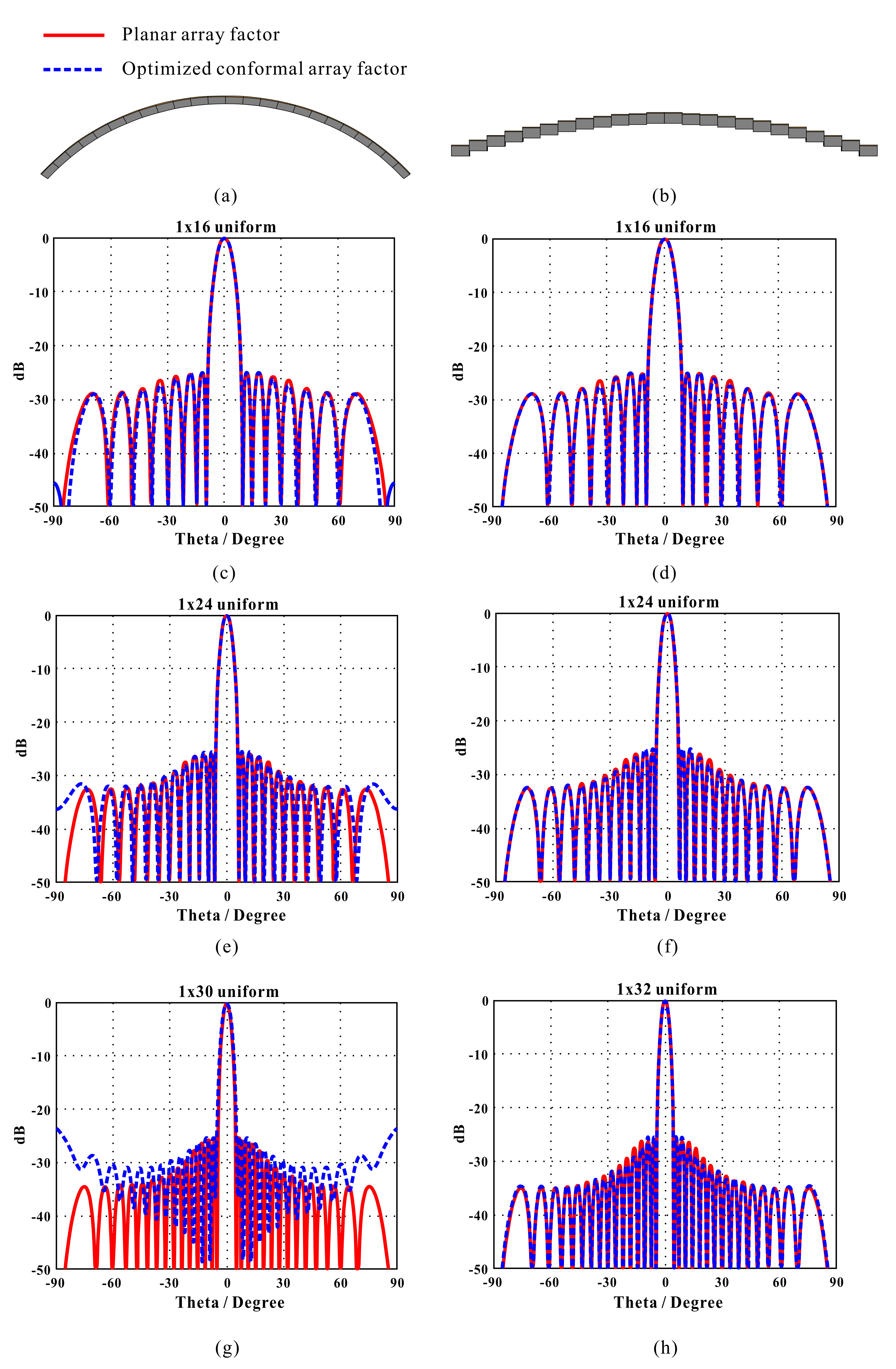
For optimization, the element positions of 1$\times$16, 1$\times$24, 1$\times$30, and 1$\times$32 conformal arrays were used. All arrays had an x-direction element spacing of dx = 0.5$\lambda$ (15 mm) at 10 GHz, and the z-direction element spacing dz was randomly set. The array factors were calculated using MATLAB for the given arrays and compared with the −25 dB Taylor array factor using the Taylor distribution for the planar arrays. The cost function used to optimize the array factor is the same as Equation (13).

$$\begin{array}{c}costfunction(SL{L}_{target}=-25)={|SL{L}_{target}-FirstSidelobelevel|}^3\\ +|SL{L}_{target}{-SecondSidelobelevel|}^2\\ +max{(-SL{L}_{target}+Sidelobelevel,(SL{L}_{target}-10)-Sidelobelevel)}^2\end{array}$$

(13)

The optimization cost function was set as follows, because the SLL values of the first and second SSLs are very close to the SLL value of the desired level, and other SLLs were set to naturally have SLLs within a certain value.

Figure 9 shows a plot of the array factors with respect to the optimized Bernstein polynomial variable. In the array factor graph, it can be seen that the array factor of a linear array with the same number of elements is similar to that of a conformal array. Analyzing the output data after verifying the performance of GLPSO and validity of the cost function, we confirmed that $N_0$ and $N_1$ correspond to a certain curvature, and the number of elements is fixed. When c changes, it has a specific inflection point and can be expressed generally for a value of c above a specific inflection point. Figure 10 shows the changes in $c_0$ and $c_1$ when dx = 0.5$\lambda$ (15 mm), dz is randomly set to a 1$\times$16 conformal array at 10 GHz, and $N_0$ = $N_1$ = 5. (Since it is a symmetric structure, we assume that $c_0$ = $c_1$ = c.)

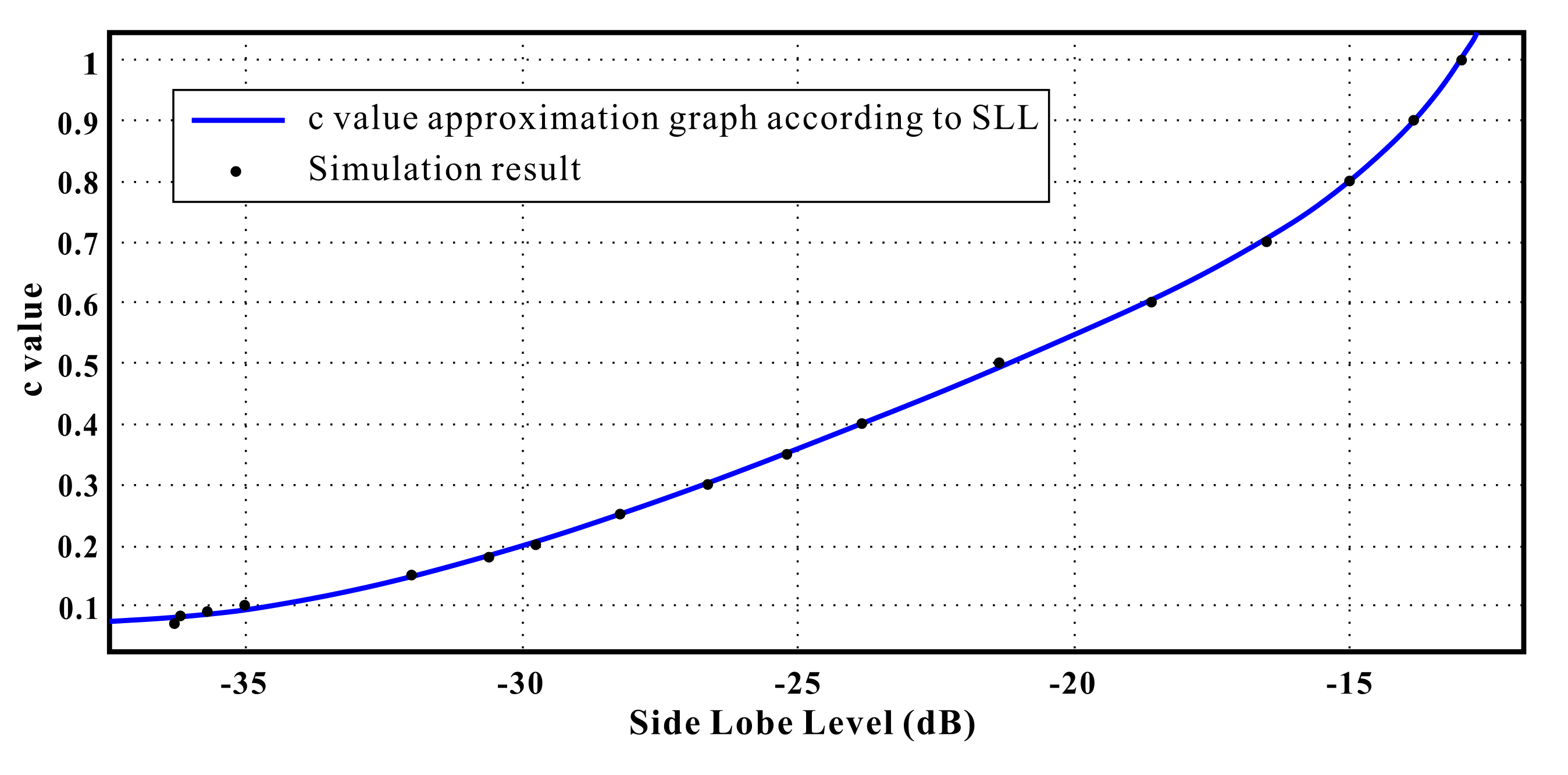
By arranging the experimentally obtained data in Figure 10, we find that the case of a 1$\times$16 conformal array can be approximated as a function of c-value according to SLL (Figure 11). We obtain an expression by analyzing the trend of the optimization results that fit the array case. Based on this, for a specific conformal array, the relation between c and SLL can be obtained based on $N_0$ and $N_1$, which are obtained through optimization.

Figure 12a shows the actual shape of the 1$\times$16 conformal array used for the CST simulation based on the information used for the MATLAB optimization. Figure 12b compares the radiation pattern of the conformal array without beam scanning and the planar-array radiation pattern to observe only the amplitude effect. The red solid line indicates dx = 0.5$\lambda$ (15 mm) for the 1$\times$16 planar array at 10 GHz and the radiation pattern when −25 dB Taylor distribution is applied. The blue dash line indicates dx = 0.5$\lambda$ (15 mm) at 10 GHz, and dz represents the randomly set 1$\times$16 conformal array radiation pattern. Variables of the Bernstein polynomial applied to the 1$\times$16 conformal array were set to $N_0$ = $N_1$ = 5, $c_0$ = $c_1$ = 0.3 according to the expressions obtained above, and Figure 11 shows that the first SLL is −26.5 dB. Simulation results show that the first SLL is −26.57 dB in the case of conformal arrays (Figure 12b), which is comparable to −26.5 dB. In addition, the radiation pattern of the 1$\times$16 planar array shows a decreasing trend with similar values, not only the shape of the pattern and the first SLL, but all SLL values.

Figure 11 and the simulated radiation patterns (Figure 12b) confirm that it is possible to derive a conformal-array amplitude tapering relationship that can be universally used depending on the situation through optimization results and variable control.

3. Discussion

We verify the proposed phase-compensation-based calculation method and amplitude tapering through simulations. We used the 8$\times$8 random grid array in Figure 7 with the cavity-backed patch antenna operating at 10 GHz. For the array factor, Equation (10) was used, with $\varphi$ = 0${}^{\circ }$, $\theta$ = 30${}^{\circ }$ beam scanning. Amplitude tapering was obtained by deriving the values of $N_0$, $N_1$, and c, and SLL was −25 dB for the 1$\times$8 conformal array, based on the expression in Section 2.3, and multiplying them by assigning amplitudes in the x- and y-directions.

Figure 13 shows the obtained amplitude curve applied to the actual x-direction. A = 0.5, $N_0$ = $N_1$ = 3 is set, and c is set as $c_0$ = $c_1$ = 0.3563, which is −25 dB for the first SLL based on Figure 11.

Figure 14a shows the $\varphi$ = 0${}^{\circ }$-plane (XZ plane) array factor pattern of a 8$\times$8 conformal array obtained by the phase compensation method and the expression based on the optimization data. Figure 14b shows the $\varphi$ = 0${}^{\circ }$-plane 2D radiation pattern of the 8$\times$8 random grid array to which the calculated amplitude and phase and uniform feeding with amplitude tapering are applied. The pattern shown in Figure 14a is similar to that of an 8$\times$8 planar array with dx = 0.5$\lambda$ (15 mm) and dy = 0.5$\lambda$ (15 mm) on the left side of $\theta$ = 30${}^{\circ }$, except for $\theta$ = −90${}^{\circ }$. The SLL is higher than that on the right side of $\theta$ = 30${}^{\circ }$. This is because SLL is relatively high due to beam scanning and the reduction in the gain of the main beam due to the structure and nonperiodicity. For the simulated radiation pattern (Figure 14b), SLL near the right side of $\theta$ = 30${}^{\circ }$ and at $\theta$ = −90${}^{\circ }$, which were high due to the effect of the element pattern in Figure 6c, decreased. Compared with the uniform feeding pattern, the first SLL decreased from −11.4 to −21.3 dB. The SLL applied in the actual array factor was −25 dB, which changed to −21.3 dB depending on the error in the developed relationship, difference in structure, and application of element patterns. We confirmed that the phase was calculated based on Equation (8) using the element locations, and the $A{F}_{3D}$ amplitude in Equation (10) could be predicted from the optimization results. Thus, we can predict and control an adjacent pattern having an SLL similar to that of the desired pattern for an arbitrary 3D array without repeated optimization.

4. Conclusions

Based on previous studies, we discussed a universal approach for calculating array factors in the form of 3D random arrays, including conformal arrays. We propose an amplitude relational method based on Bernstein polynomial optimization and phase compensation. The proposed phase calculation method is not limited to specific grid structures (e.g., rectangular and triangular grids), but it is widely applicable to any 3D phased array. Unlike previous studies on phase compensation in conformal arrays, the method does not require different expressions for different structures; rather, one expression can be used for any 3D structure. The proposed phase calculation method was verified by simulating uniform amplitude feeding using an 8$\times$8 random array of a cavity-backed patch antenna operating at 10 GHz. Next, we developed a relationship between amplitude tapering and phase compensation by analyzing the results obtained using GLPSO in the Bernstein polynomial. Unlike previous studies on conformal array amplitudes, optimization is not performed for different element shapes, array shapes, and radiation patterns; rather, an expression is developed based on the optimization results obtained in a case with which the amplitude for the radiation pattern is quickly derived. The proposed method needs to be improved as optimization is not performed each time to obtain the best results in each case, as in previous studies. However, universal equations can be derived, and prediction and control of the performance of patterns for arbitrary 3D arrays can be achieved in a short time. To verify the proposed method, we applied phase compensation and amplitude tapering to an array and verified the performance through simulations. Future work will involve the fabrication of the proposed cavity-backed patch antennas and its implementation in an 8$\times$8 random grid array system for experimental verification. The 8$\times$8 random grid array shown in this paper can be measured by manufacturing a metal jig that matches the shape of the array. To date, studies are ongoing to develop and commercialize conformal arrays. Based on our results herein and those of previous studies, a universal array factor can be obtained for all array types through phase compensation and amplitude tapering for conformal arrays. For all phased arrays (such as planar and conformal arrays), mathematical and beam synthesis methods can be developed to control SLL without the need for optimization for each case.

References

1. Josefsson, L.; Persson, P. Conformal Array Antenna Theory and Design; John Wiley & Sons: Hoboken, NJ, USA, 2006; Volume 29. [Google Scholar]
2. Boeringer, D.W.; Werner, D.H. Efficiency-constrained particle swarm optimization of a modified Bernstein polynomial for conformal array excitation amplitude synthesis. IEEE Trans. Antennas Propag. 2005, 53, 2662–2673. [Google Scholar] [CrossRef]
3. Braaten, B.D.; Roy, S.; Irfanullah, I.; Nariyal, S.; Anagnostou, D.E. Phase-compensated conformal antennas for spherical surfaces. IEEE Trans. Antennas Propag. 2014, 62, 1880–1887. [Google Scholar] [CrossRef]
4. Hizal, A. Wide angle scanning conformal phased array on a spherical surface. In Proceedings of the 2013 IEEE International Symposium on Phased Array Systems and Technology, Waltham, MA, USA, 15–18 October 2013. [Google Scholar]
5. Zeng, Y.; Zhang, S.; Li, N.; Duan, B.; Yi, Q.; Zhang, J.; Sun, Z. Shaped Elevation Beam Design for Airborne Conformal Array Detection. IEEE Antennas Wirel. Propag. Lett. 2020, 19, 2192–2196. [Google Scholar] [CrossRef]
6. Jorna, P.; Schippers, H.; Verpoorte, J. Beam synthesis for conformal array antennas with efficient tapering. In Proceedings of the 5th European Workshop on Conformal Antennas, Bristol, UK, 10–11 September 2007. [Google Scholar]
7. Boeringer, D.W.; Werner, D.H. Bezier repersentations for the multiobjective optimization of conformal array amplitude weights. IEEE Trans. Antennas Propag. 2006, 54, 1964–1970. [Google Scholar] [CrossRef]
8. Aslan, Y.; Roederer, A.; Yarovoy, A. Synthesis of Low-Sidelobe Stepped-Amplitude Aperiodic Phased Arrays. In Proceedings of the 2021 15h European Conference on Antennas and Propagation (EuCAP), Dusseldorf, Germany, 22–26 March 2021. [Google Scholar]
9. Bekele, E.T.; Oliveri, G.; Turpin, J.P.; Werner, D.H.; Massa, A. Design of metamaterial-coated arrays through quasi-conformal transformation optics. In Proceedings of the 8th European Conference on Antennas and Propagation (EuCAP 2014), The Hague, The Netherlands, 6–11 April 2014. [Google Scholar]
10. Brown, A.D. (Ed.) Electronically Scanned Arrays MATLAB® Modeling and Simulation; CRC Press: Boca Raton, FL, USA, 2017. [Google Scholar]
11. Choi, D.S.; Choi, Y.S.; Jeong, J.Y.; Jung, T.H.; Woo, J.M. Four-Array Printed Monopole Yagi-Uda Antenna Mounted on a Small Missile Warhead. J. Electromagn. Eng. Sci. 2021, 21, 143–147. [Google Scholar] [CrossRef]
12. Ellgardt, A.; Wikstrom, A. A single polarized triangular grid tapered-slot array antenna. IEEE Trans. Antennas Propag. 2019, 57, 2599–2607. [Google Scholar] [CrossRef]
13. Jang, D.; Hur, J.; Shim, H.; Park, J.; Cho, C.; Choo, H. Array antenna design for passive coherent location systems with non-uniform array configurations. J. Electromagn. Eng. Sci. 2020, 20, 176–182. [Google Scholar] [CrossRef]
14. Jung, S.H.; Lee, K.I.; Oh, H.S.; Jung, H.K.; Yang, H.; Chung, Y.S. Optimal Design of Thinned Array Using a Hybrid Genetic Algorithm. J. Electromagn. Eng. Sci. 2021, 21, 261–269. [Google Scholar] [CrossRef]
15. Kwon, D.-H. Quasi-conformal transformation optics lenses for conformal arrays. IEEE Antennas Wirel. Propag. Lett. 2012, 11, 1125–1128. [Google Scholar] [CrossRef]
16. Nam, J.H.; Rim, J.W.; Lee, H.; Koh, I.S.; Song, J.H. Modeling of monopulse radar signals reflected from ground clutter in a time domain considering Doppler effects. J. Electromagn. Eng. Sci. 2020, 20, 190–198. [Google Scholar] [CrossRef]
17. Gong, Y.J.; Li, J.J.; Zhou, Y.; Li, Y.; Chung, H.S.; Shi, Y.H.; Zhang, J. Genetic learning particle swarm optimization. IEEE Trans. Cybern. 2015, 46, 2277–2290. [Google Scholar] [CrossRef] [PubMed] [Green Version]
18. Hur, J.; Choo, H. Design of a small array antenna with an extended cavity structure for wireless power transmission. J. Electromagn. Eng. Sci. 2020, 20, 9–15. [Google Scholar] [CrossRef]
19. Nakano, H.; Iwatsuki, M.; Sakurai, M.; Yamauchi, J. A cavity-backed rectangular aperture antenna with application to a tilted fan beam array antenna. IEEE Trans. Antennas Propag. 2003, 51, 712–718. [Google Scholar] [CrossRef]
20. Yun, J.; Trinh-Van, S.; Park, J.Y.; Yang, Y.; Lee, K.Y.; Hwang, K.C. Cavity-Backed Patch Filtenna for Harmonic Suppression. IEEE Access 2020, 8, 221580–221589. [Google Scholar] [CrossRef]
Figure 1. Single element information used for conformal-array characteristic analysis: (a) element type, (b) S-parameters information.
Applsci 12 06501 g001
Figure 2. Description of array type and related variables: (a) 12 × 24 planar array, (b) 12 × 24 conformal array, (c) description of variable r.
Applsci 12 06501 g002
Figure 3. Comparison of 2D radiation patterns of 12 × 24 planar and conformal arrays: (a) ϕ = 0 plane and (b) ϕ = 90 plane.
Applsci 12 06501 g003
Figure 4. Arrangement shape on the XZ plane: (a) linear array (planar array) shape and (b) curved array (conformal array) shape.
Applsci 12 06501 g004
Figure 5. Detailed locations of conformal array elements.
Applsci 12 06501 g005
Figure 6. Cavity-backed patch antenna: (a) element shape, (b) S-parameters, (c) ϕ = 0 radiation pattern and (d) ϕ = 90 radiation pattern.
Applsci 12 06501 g006
Figure 7. 8 × 8 random grid array shape: (a) 3D view and (b) XY plane view.
Applsci 12 06501 g007
Figure 8. Comparison of 8 × 8 random grid array uniform feeding 2D radiation patterns: (a) array factor of conformal array calculated using MATLAB and (b) radiation pattern from EM simulation.
Applsci 12 06501 g008
Figure 9. Array factors (−25 dB) of conformal array optimized based on GLPSO: (a) conformal array type 1; (b) conformal array type 2; comparison of radiation patterns of (c) 1 × 16 conformal array type 1 and 1 × 16 planar array, (d) 1 × 16 conformal array type 2 and 1 × 16 planar array, (e) 1 × 24 conformal array type 1 and 1 × 24 planar array, (f) 1 × 24 conformal array type 2 and 1 × 24 planar array, (g) 1 × 30 conformal array type 1 and 1 × 30 planar array, and (h) 1 × 32 conformal array type 2 and 1 × 32 planar array.
Applsci 12 06501 g009
Figure 10. Relation graph between sidelobe level and variable c of Bernstein polynomial.
Applsci 12 06501 g010
Figure 11. Approximate graph of c -value according to sidelobe level.
Applsci 12 06501 g011
Figure 12. Application of the calculated amplitude based on the optimization trend: (a) conformal array shape with amplitude applied and (b) 1 × 16 conformal array radiation pattern vs. linear array radiation pattern.
Applsci 12 06501 g012
Figure 13. Amplitude tapering curves applied to actually validation cases.
Applsci 12 06501 g013
Figure 14. Comparison of 8 × 8 random-grid amplitude-tapering 2D radiation patterns: (a) array factor of conformal array calculated with MATLAB, (b) comparison of simulated radiation patterns for uniform and amplitude tapering feeding.
Applsci 12 06501 g014
Publisher’s Note: MDPI stays neutral with regard to jurisdictional claims in published maps and institutional affiliations.