Design and Implementation of an Explainable Bidirectional LSTM Model Based on Transition System Approach for Cooperative AI-Workers

Abstract

Recently, interest in the Cyber-Physical System (CPS) has been increasing in the manufacturing industry environment. Various manufacturing intelligence studies are being conducted to enable faster decision-making through various reliable indicators collected from the manufacturing process. Artificial intelligence (AI) and Machine Learning (ML) have advanced enough to give various possibilities of predicting manufacturing time, which can help implement CPS in manufacturing environments, but it is difficult to secure reliability because it is difficult to understand how AI works, and although it can offer good results, it is often not applied to industries. In this paper, Bidirectional Long Short Term Memory (BI-LSTM) is used to predict process execution time, which is an indicator that can be used as a basis for CPS in the manufacturing process, and the Shapley Additive Explanations (SHAP) algorithm is used to explain how artificial intelligence works. The experimental results of this paper, applying manufacturing data, prove that the results derived from SHAP are effective for workers and AI to collaborate.

1. Introduction

In the recent manufacturing industry environment, with Digital Transformation (DT) [1] that combines digital technology and business models to create great value, manufacturing intelligence has become the biggest trend. At the same time, interest in Cyber-Physical Systems (CPS) is increasing [2]. In Industry 4.0, the development of information and communication is digitizing the industrial environment, improving the industrial system into an autonomous system that can make autonomous decisions through the CPS. As a result, industry can lower production costs by improving logistics and productivity [3]. As manufacturing systems become more complex to adapt to rapid changes in consumption trends, interest in CPS is increasing [4]. CPS, which also enables real-time prediction, monitoring, optimization, and control, is currently a key pillar of Industry 4.0 to turn the manufacturing industry into a fully automated smart factory [5].

Machine Learning (ML) and Artificial Intelligence (AI) can offer exciting new possibilities for manufacturing CPS [6]. A model can predict the quality of finished products using Auto-Regressive Integrated Moving Average (ARIMA), which is machine learning [7]. A recent study has proven that Long Short-Term Memory (LSTM) is suitable for predicting inventory supply and demand in the manufacturing process [8]. There are also various attempts to use Bidirectional Long Short Term Memory (BI-LSTM) for intelligent manufacturing. Research results have shown that valid results can be obtained when BI-LSTM is applied to the life expectancy model of manufacturing equipment [9]. In addition, another study proved that BI-LSTM is suitable for predicting the damage tendency of bearings [10].

However, there are clear challenges to adopting these technological solutions. It is difficult to understand how AI works, which causes a lack of trust in AI; while AI can provide positive results for the manufacturing industry, its immediate application to industry is not easy. In particular, in the manufacturing environment, AI can show good performance in predicting manufacturing time based on real-time data [11], and we wanted to extend this model to an Explainable Artificial Intelligence (XAI) model. We want to provide a CPS-based AI collaboration framework through which AI and workers can collaborate by enabling operators and workers to understand AI judgments. In this paper, we devise a CPS model that predicts the remaining manufacturing time by analyzing the manufacturing machine operating time using process mining technology. We propose a possible cooperative architecture. Our study offers three main contributions:

(1)

We propose a transition-based data preprocessing method that utilizes log data applied with process mining technology. This data processing technology can help interpret the manufacturing process data generated by manufacturing companies.

(2)

In order to apply AI-based CPS to actual processes, it is necessary to solve the black box characteristic, the biggest problem of AI. This paper can improve the reliability of AI by solving these black box characteristics. In addition, AI interpretation requires a lot of technology and labor costs, and in the case of small and medium-sized enterprises, it is difficult to continuously receive help from experts due to cost problems.

(3)

In this paper, using SHAP to solve this problem, we can try to analyze AI more simply and effectively, and through actual manufacturing environment data, we prove that the output of SHAP is helpful in solving the black box characteristics of AI.

The rest of the thesis is structured as follows. Section 2 introduces process mining research applicable to the CPS. Section 3 describes the components of the approach proposed in the text, the main ideas of the study, the proposed transition system-based data preprocessing model, and the XAI method. Section 4 describes the experimental environment, the structure of the data set, and the experimental results. Section 5 concludes the paper with a summary of the paper, evaluation results, and future research directions.

2. Related Work

2.1. Digital Twin and CPS

In recent years, the number of devices connected to the local network and the Internet to form an intelligent system has increased significantly. This, in turn, aims to improve efficiency, agility, and user experience and support more autonomous decision-making [12]. In addition, these advances in information and communication technology have made it possible to collect and verify more detailed field data in real-time [13]. Using such data, the manufacturing environment is projected into virtual space to create a digital twin that reflects reality, the manufacturing process operation decision is made in that space, and the method of making operational decisions using big data evolves [14]. Recently, in addition to the CPS that enables real-time distributed control systems, research on digital twins, defined as virtual representations of physical assets created through data and simulators, continues. In Industry 4.0, the CPS and the digital twin are considered the key factors [15]. In particular, the digital twin creates a digital process based on physical process information in cyberspace and conducts learning for optimal process operation control by analyzing the movement of machines in the manufacturing process. In addition, by building CPS on the actual manufacturing process machine, the learning results obtained from the digital twin can be autonomously applied to industrial machines to strengthen collaboration between the real and virtual, and make the production process more flexible. As such, the connection between digital twins and CPSs can create strong synergies [16]. To support autonomous processes, data obtained from industrial processes must be processed quickly and accurately, and AI is a representative technology that can support the complete automation of the manufacturing process [17]. Existing systems in which people think, create, and adjust according to the manual are difficult to adapt to the dynamic environment that changes at a very fast rate [18]. In addition, to analyze the data of each process and place an accurate order for it in a timely manner, experienced consultants and managers are needed in real-time, which is expensive. Various recent studies on AI have shown that an automatic system can be implemented and show the possibility of it actually being used in the manufacturing field. Such smart manufacturing has a strong competitive edge in Industry 4.0 [19]. However, the adoption of AI technology has the drawback that it is difficult to understand and apply to actual processes due to the opacity of the decision [20].

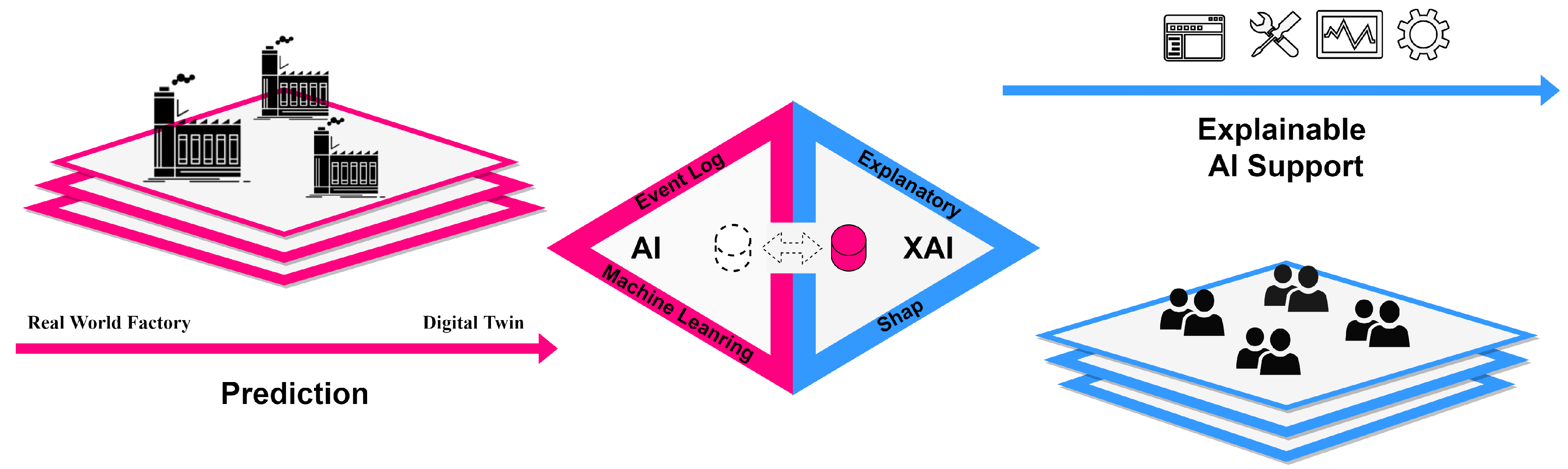
Figure 1 visually expresses the AI cooperation framework. Based on actual manufacturing process data, a digital twin is created in the virtual world, and the collected static operation data are learned through an AI algorithm to analyze the optimal operation scenario. Then, based on the CPS, it gives commands to the distributed actual process to solve problems, such as bottlenecks, that may occur in the manufacturing process. It provides explainable AI assistance to the worker to help them understand the behavior and consequences of the AI. Process operators can benefit from these comments to make faster and more accurate decisions [21].

Figure 1. AI cooperation framework.

2.2. XAI Technologies

Modern implementations of the CPS and digital twin are moving away from the traditional consultative approach to a machine learning approach that results from learning process data. It is difficult to adapt to the environment in response to the rapidly changing market demand in the existing method of analysis by humans [18]. However, AI also has chronic problems. Since it is not easy to understand how AI works, the black box characteristics of AI lower its reliability and cause many difficulties in applying it to actual processes. Many studies are being conducted to solve this problem. XAI is a field of research that aims to make the results of AI systems easier for humans to understand [22]. The term was first coined by Van Lent in 2004 to describe the ability of a system to describe the behavior of AI-based entities in simulation games. Although the term was only coined relatively recently, the problem of ‘explainability’ has existed since the mid-1970s, when explanations of expert systems were studied. However, since then, AI and ML have developed rapidly, and as AI research places more importance on predictive power than decision-making processes, interest in explanatory power has declined. Recently, it has been receiving renewed attention from academia and practitioners, because as AL/ML penetrates the industry, the influence of AL/ML on decision-making is becoming more important. Accordingly, there is a demand for AI technology that can be explained ethically, socially, and legally.

The necessity of XAI research can be explained in four ways, as shown in Figure 2.

Figure 2. The need for XAI.

-

Justify: Over the past few years, there has been debate about whether AI/ML-based systems are discriminatory or biased. This indicates a growing need for explanations to ensure that AI-based decisions are not made incorrectly. This refers to the need to provide a reason or justification for a particular outcome rather than an explanation of the inner workings of the decision-making process [23].

-

Control: The better the understanding of the behavior of a system, the greater the visibility into its vulnerabilities and flaws, and the faster that errors can be fixed, providing greater control [22].

-

Improve: A model that can be explained and understood can be more easily improved. Knowing why a particular output was generated can make the system more sophisticated.

-

Discover: Explanations are needed to learn new facts and gather information. Considering that AI can be superior to humans, if AI can explain the strategies or knowledge it has learned to humans, AI can also inform humans of new laws of natural science that humans are not aware of.

Techniques that explain XAI can be divided into two broad categories, feature-based technology and example-based technology. Feature-based technology describes how input features affect the model’s output, and example-based technology describes how examples affect the model’s output. Representatively, feature-based technologies include Local Interpretable Model-agnostic Explanations (LIME) and SHAP, and example-based technologies include Contrastive Explanation Method (CEM) and Kernel SHAP [24].

The recent success of AI stems in large part from advances in ML algorithms that include SVM, random forest, reinforcement learning, and Deep Learning (DL) models. In particular, research on DL has been actively conducted and has been successfully used in various fields, such as medicine, ophthalmology, autonomous robotics, image processing, and voice and audio processing. However, there is the problem that these AI systems cannot explain their internal mechanisms. The performance (predictability) and explainability of ML are an intrinsic conflict. For example, the best performing DL is the most difficult to explain, and the easiest to explain the decision tree is the least accurate. When it comes to using AI systems in critical industries, such as medicine, defense, finance, and law, leaving decisions to systems that cannot explain how they work presents obvious risks. For users to understand, trust, and effectively manage AI systems, explainability is essential, which has made the XAI of AI an important issue.

2.3. Event Log

In the recent market, consumption trends change very quickly; the demand for products optimized for individuals is increasing, and the desire for customization is increasing. It is very difficult to adapt the manufacturing process to ever-changing consumption trends, and it requires flexibility in the manufacturing process. To adapt to these rapid changes, the traditional method that relies only on expert experience and consultants, such as the existing method, is changing to a method that utilizes AI that can use data-driven technology using big data in recent research [25]. In particular, research on process mining technology that analyzes and discovers the next process by tracking sequenced data is being actively conducted [26]. Process mining can analyze the cause by tracking the change in the result according to the process result or the change in the intermediate process. Processes and their relationships can also be analyzed [27]. Previous studies have shown that process mining techniques are effective in using decision tree techniques to uncover the reasons for bottlenecks in manufacturing processes ferreira2015using.

Process mining technology can help explain the correlation between processes, as demonstrated by previous studies, and can also be introduced into manufacturing processes. In fact, according to the development of information and communication technology in the manufacturing process, data are rapidly accumulating through various equipment, and big data are being generated. However, because it is very complex to use big data [28], the technology of SMEs is still insufficient to use big data, and the human resources of SMEs are grossly insufficient to obtain new insights by relying on the experience of consultants and experts, which are traditional methods. Table 1 shows an example of the log data that are constantly accumulated in the manufacturing process. A case number is given, and it is accumulated sequentially according to the change of activity. To track the process, various information is included, such as start time and end time, and the type and number of products. Each case means a separate process, and this is valuable information that can reveal the correlation between processes in the manufacturing process through various kinds of data.

Table 1. Example of an event.

Case ID	Start Time	End Time	Product	Machine	Qtty
Case01	01-20-2022: 11:00	01-20-2022: 11:10	A	1	5
Case01	01-20-2022: 11:20	01-20-2022: 11:40	A	2	5
Case01	01-20-2022: 11:55	01-20-2022: 12:10	A	3	5
Case01	01-20-2022: 12:30	01-20-2022: 12:40	A	4	5
Case02	01-20-2022: 13:00	01-20-2022: 13:20	B	1	20
Case02	01-20-2022: 13:30	01-20-2022: 13:40	B	3	20
Case02	01-20-2022: 14:10	01-20-2022: 14:30	B	2	20
Case02	01-20-2022: 14:50	01-20-2022: 16:00	B	4	20
Case03	01-20-2022: 08:00	01-20-2022: 08:35	A	1	5
Case03	01-20-2022: 08:40	01-20-2022: 09:10	A	3	5
Case03	01-20-2022: 09:25	01-20-2022: 09:40	A	2	5
Case03	01-20-2022: 10:10	01-20-2022: 10:55	A	4	5
Case04	01-20-2022: 06:00	01-20-2022: 06:30	B	1	10
Case04	01-20-2022: 06:40	01-20-2022: 07:10	B	2	10
Case04	01-20-2022: 07:30	01-20-2022: 07:50	B	3	10
Case04	01-20-2022: 08:10	01-20-2022: 08:30	B	4	10

Table 1 above, as in the event log data described above, each case has a case ID; each case exists individually and is sequentially recorded according to the start time and end time. Each Case ID has machine information passed through the process and also includes the number of productions according to the product. Process mining technology can track each process by classifying and analyzing these Case IDs, and process mining technology is frequently dealt with in recent smart factories, as in [29], in which the authors wanted to predict the manufacturing system, tried to understand the correlation between each manufacturing process through process mining technology, and proved that it could. This paper aims to provide reliable AI results by learning artificial intelligence using event log data and implementing explainable artificial intelligence so that it can adapt to the changing environment more flexibly and autonomously.

2.4. Bi-LSTM

BI-LSTM is a method of adding a reverse LSTM layer to the existing forward LSTM layer, so that the final hidden state outputs a vector connecting the hidden state between the two LSTM layers. This reverse vector captures the hidden properties and patterns of data that have been ignored in general LSTMs. This allows the surrounding information for each hidden state to be balanced in both directions and solves the problem that the existing LSTM experiences a bottle-neck problem in which information is lost.

Bi-LSTM uses two LSTM layers and is implemented by adjusting the data order of the layers. The first layer analyzes the data pattern in the same forward direction as before, while the second layer analyzes the data pattern in the reverse direction. The overall results are analyzed by linking, adding, or averaging the results analyzed in the two directions. It is necessary to first look at the equation of Recurrent Neural Network (RNN) to represent Bi-LSTM mathematically [30]:

$$h_t=tanh\left(W_{xh}{x}_t+W_{hh}{h}_{t-1}+b_h\right)$$

(1)

$$y_t=W_{hy}{h}_t+b_y$$

(2)

where $h_t$ refers to the hidden state output in the RNN neural network [30]. W represents the weight connecting input $x_t$ to hidden layer $h_t$. The hidden layer $h_t$ is calculated by multiplying the input value x and the previous hidden layer $h_{t-1}$ by each weight and adding the bias vector b. Output layer $y_t$ is calculated by multiplying the hidden layer by the weight $W_{hy}$ and adding bias $b_y$. However, RNN has a disadvantage that when too much information is accumulated, it is difficult to continue information due to the long dependency period. To compensate for this, a new method has begun to be used. LSTM is a type of RNN, which is explicitly designed to avoid a long dependency period, allowing the model to remember information over a long period of time on its own. Although it is a chain structure such as RNN, each iteration module has a different structure [31]. Instead of a simple natural network layer, four layers are supposed to exchange information with each other in a special way.

$$f_t=\sigma \left(W_f·\left[h_{t-1},x_t\right]+b_f\right)$$

(3)

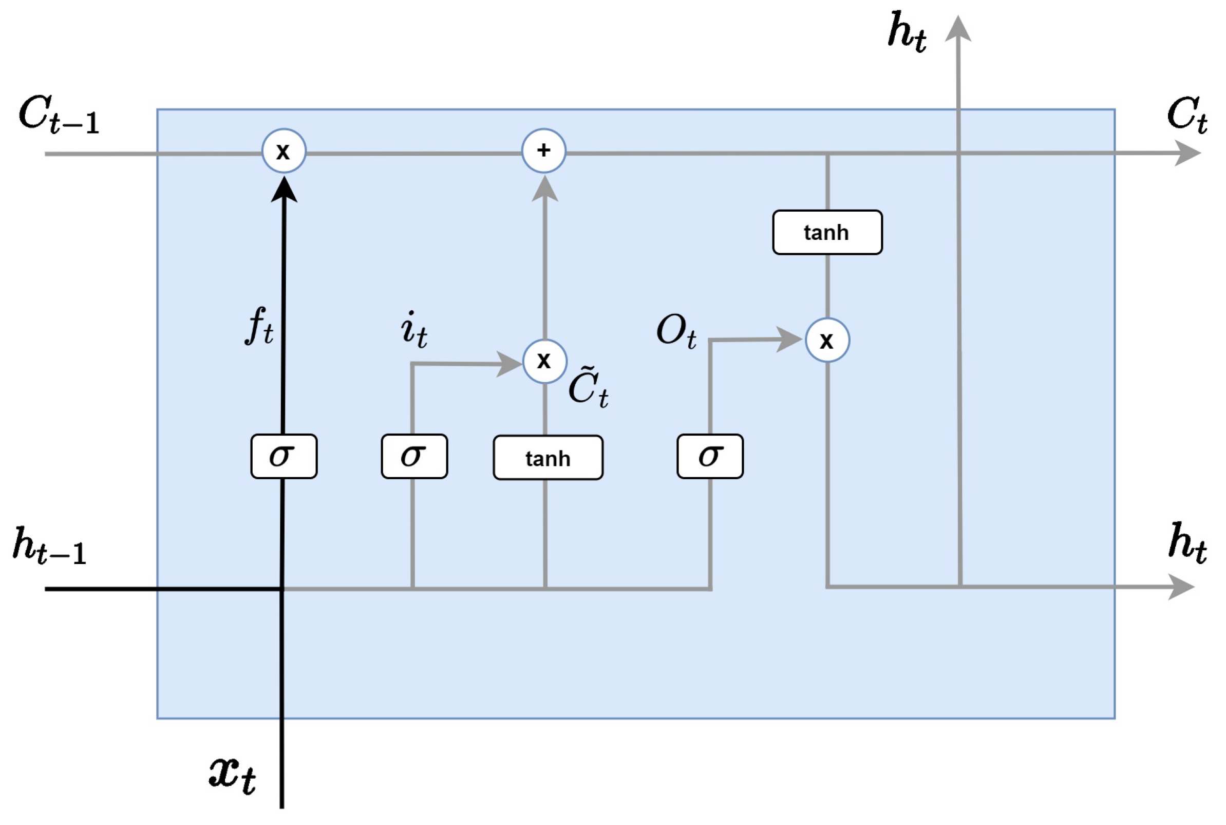
LSTM analyzes information through four main steps. As in the Figure 3, the first step is the forget gate layer, which determines which information to discard from the cell state and is determined by the sigmoid layer. At this time, the hidden state of the previous step $h_{t-1}$ and the input value $x_t$ are received, and a value between 0 and 1 is sent to $C_{t-1}$ (if the value is 1, all information is preserved). Forget $f_t$ is expressed by multiplying $h_{t-1}$ and $x_t$ by their respective weights and multiplying the sum added by the bias by the sigmoid function.

$$i_t=\sigma \left(W_i·\left[h_{t-1},x_t\right]+b_i\right)$$

(4)

$${\tilde{C}}_t=tanh\left(W_C·\left[h_{t-1},x_t\right]+b_C\right)$$

(5)

Figure 3. LSTM forget gate layer.

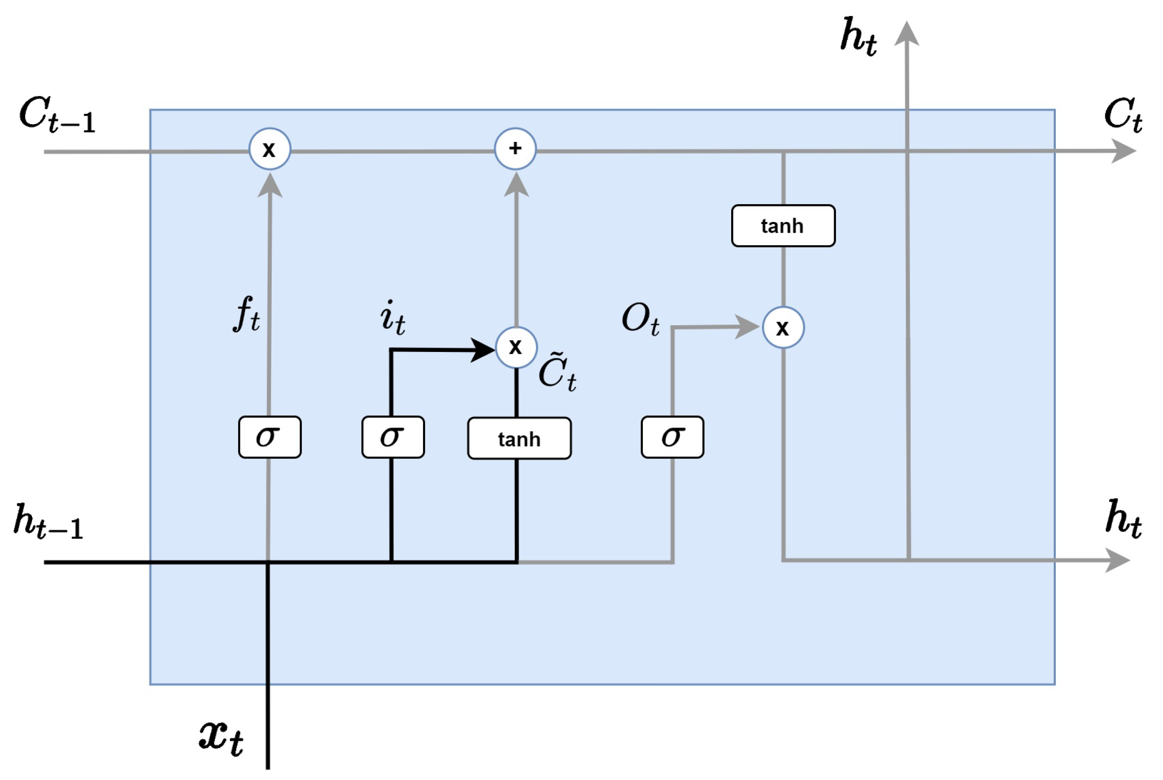
As in the Figure 4, the next step is an input gate layer, which determines which information to store among the new incoming information. First, the sigmoid layer, called the input gate layer, decides which value to update and prepares the tanh layer to add to the cell state by creating a new candidate value, ${\tilde{C}}_t$ vector. These two pieces of information will be combined to create a material to update the state.

$$C_t=f_t\ast C_{t-1}+i_t\ast {\tilde{C}}_t$$

(6)

Figure 4. LSTM input gate layer.

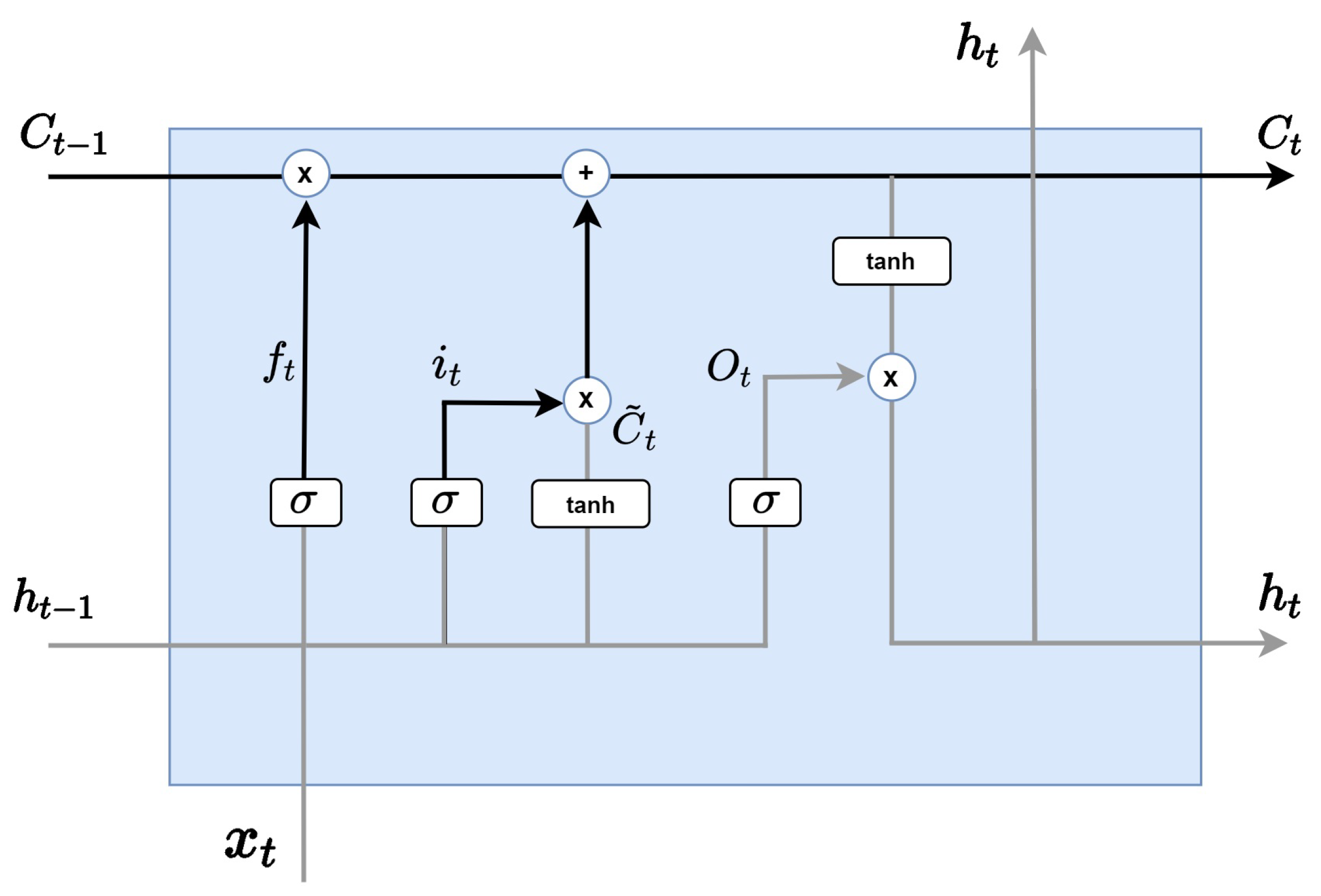
Next, As in the Figure 5, the cell state update is a step of updating the past state $C_{t-1}$ to $C_t$ by applying the previous two steps. By multiplying the previous cell state by $f_t$, the information to be erased in step 1 is forgotten, and the information to be updated is added by adding $i_t\ast {\tilde{C}}_t$. In other words, cell state $C_t$ processes deletion information by multiplying forget gate $f_t$ by the previous cell state $C_{t-1}$ and multiplying input $i_t$ by the previously calculated ${\tilde{C}}_t$ to process additional information.

$$o_t=\sigma \left(W_o\left[h_{t-1},x_t\right]+b_o\right)$$

(7)

$$h_t=o_t\ast tanh\left(C_t\right)$$

(8)

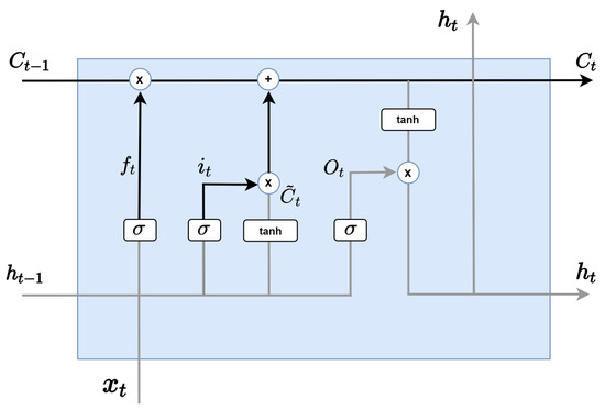
Figure 5. LSTM cell state update.

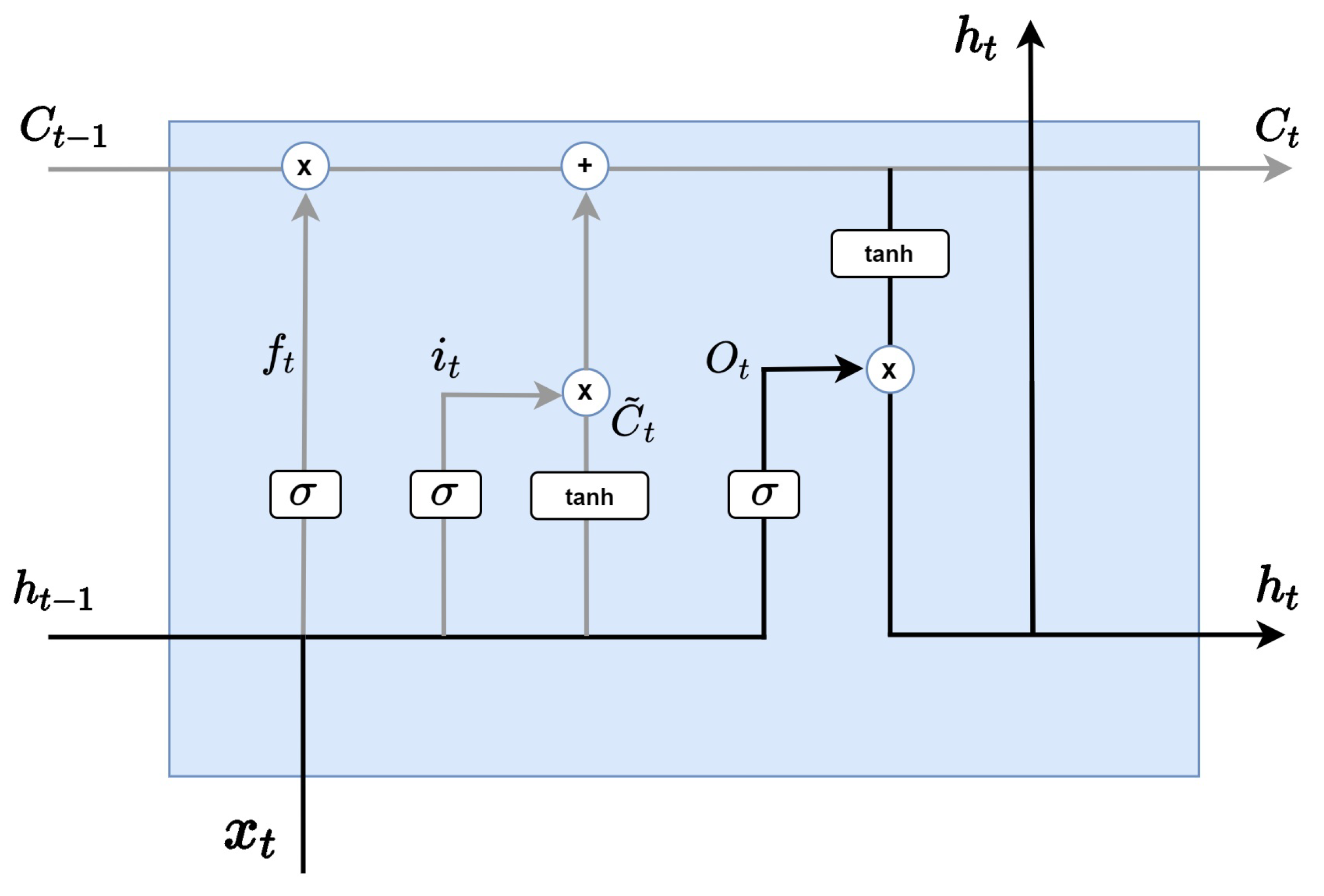
As in the Figure 6, the last step is to determine what to export to the output gate layer. First, we take input data on the sigmoid layer and decide which part of the cell state to export as output. Then, burn the cell state into the tanh layer, receive the value between −1 and 1, and multiply it by the output of the sigmoid gate that was calculated just now. Through this calculation, we can export only the part we want to send as output. Output $O_t$ is expressed by multiplying $x_t$ and $h_{t-1}$ by each weight and multiplying the sigmoid function by the sum of the value calculated and bias. Hidden state $h_t$ is represented by multiplying output $O_t$ by $tanh\left(C_t\right)$.

Figure 6. LSTM output gate layer.

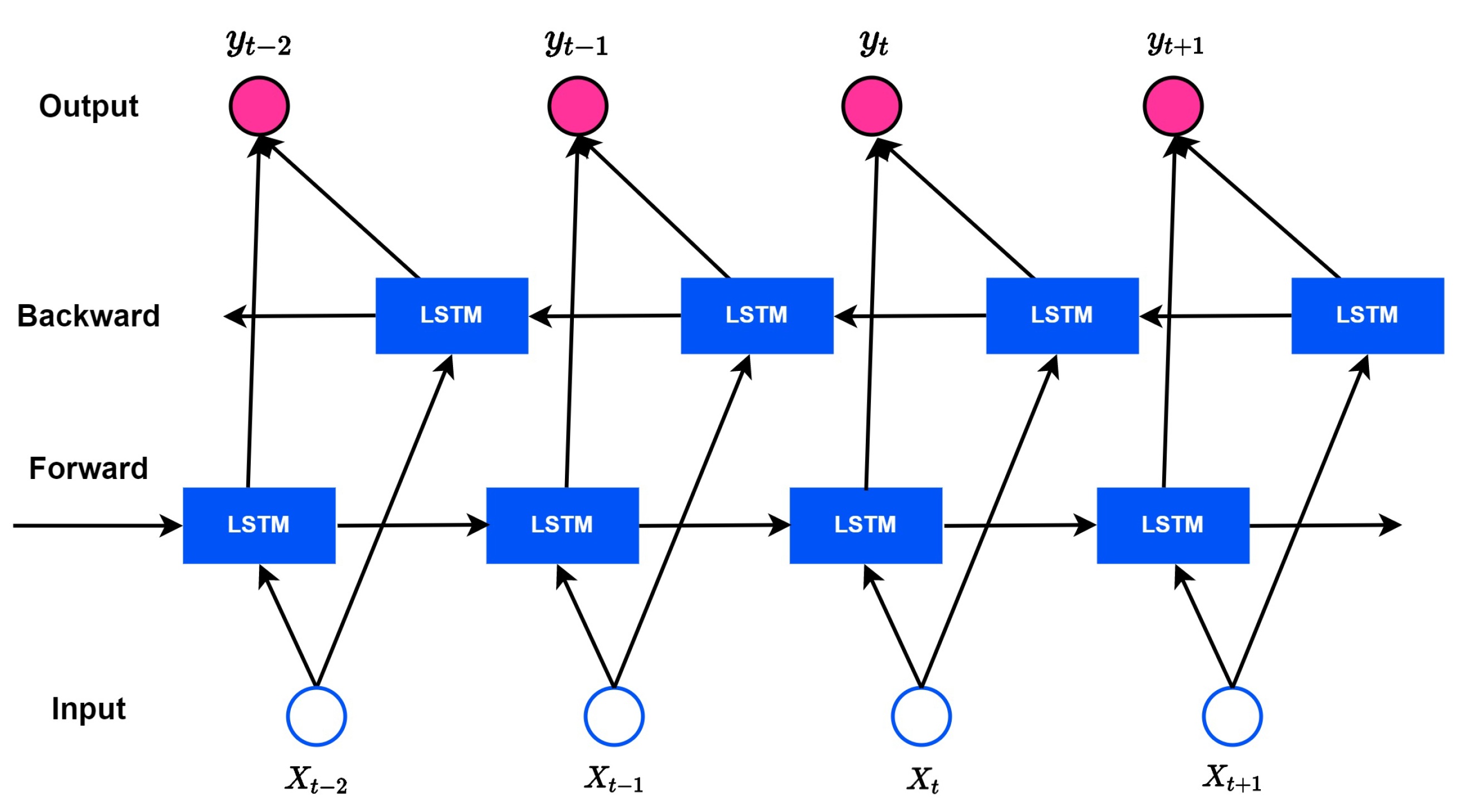
Although LSTM solves the gradient vanishing/exploding problem well, future information is not considered in the output. Therefore, As in the Figure 7, Bi-LSTM has emerged, which considers both directions of the hidden state to analyze more patterns and perform sophisticated learning by considering information in both directions. The model of Bi-LSTM is expressed as a formula, as follows:

$$h_t^f=tanh\left(W_{xh}^f{x}_t+W_{hh}^f{h}_{t-1}^f+b_h^f\right)$$

(9)

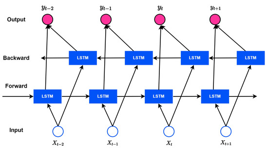
Figure 7. Overview of the BI-LSTM model.

$h_t^f$ and $h_t^b$ refer to a forward layer and a backward layer, respectively. W represents the weight connecting input x to hidden layer h.

$$h_t^b=tanh\left(W_{xh}^b{x}_t+W_{hh}^b{h}_{t+1}^b+b_h^b\right)$$

(10)

Hidden layer $h_t$ is expressed by multiplying the input value $x_t$ and the previous hidden layer $h_{t-1}$ by each weight and substituting the value obtained by adding the bias b vector into the $tanh$ function. The backup hidden layer uses a value of $h_{t+1}$ instead of $h_{t-1}$.

$$y_t=W_{hy}^f{h}_t^f+W_{hy}^b{h}_t^b+b_y$$

(11)

Output layer $y_t$ is calculated by multiplying the weight W by the hidden layer in both directions and adding bias $b_y$. By considering both hidden state values in both directions, the output value is output as a learned value not only for forward but also for backpropagation patterns. The process of calculating ${\mathcal{Y}}_t$ by adding the hidden states in both directions through the above equation is as follows. The input values in each step are input to the layers in both directions. The layers in both directions generate an $h_t$ value through the LSTM information processing process, and the two $h_t$ values are connected to the output $y_t$ of each step. Bi-LSTM minimizes the loss to output, and end-to-end learning is performed to simultaneously learn all parameters in both directions. Thus, more sophisticated models can be built than traditional LSTMs. In addition, the similarity between each input and existing patterns can be embedded in the input vector $i_t$ to improve the performance of the model, and the long data length does not degrade using the underlying performance and attention mechanism of LSTM.

3. Cooperative AI-Workers

3.1. System Architecture

This paper implements a digital twin that can predict the manufacturing process time through event log data. In addition, when applied to the factory floor through the CPS, XAI technology provides a framework that can lead to collaboration between AI and workers, enabling faster decision-making in manufacturing process operations.

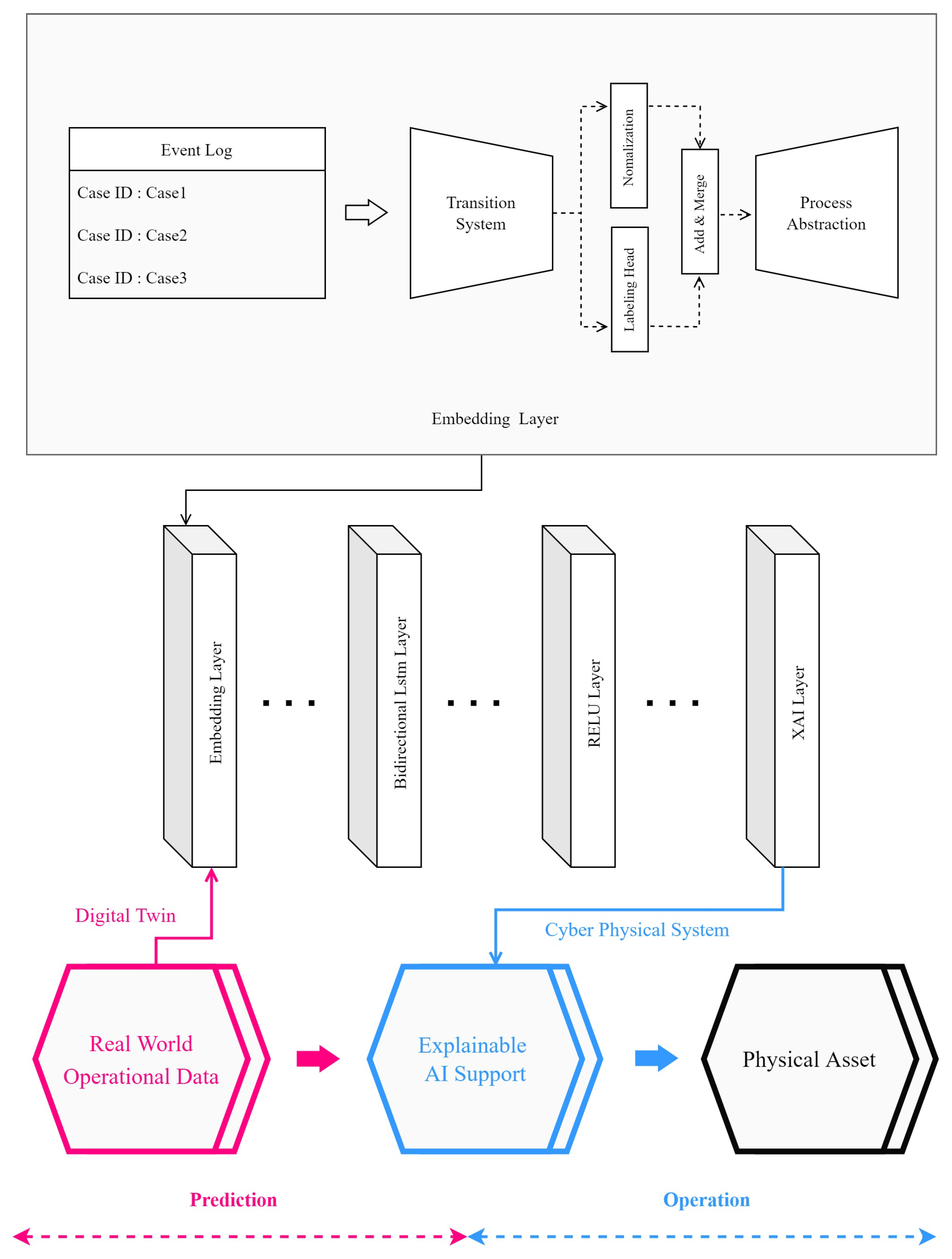
Figure 8 reflects the learning and prediction results using the AI algorithm in the real world through CPS and adding specific interpretations of the AI analysis results to enable field workers and AI to cooperate. This paper traces the process through event log data and preprocesses the collected data using a transition system. After that, the manufacturing process time is analyzed and learned using BI-LSTM, and the predicted result is interpreted and analyzed in explanatory form so that the operator can intuitively understand it through the XAI layer. We propose a mutual collaboration framework that controls the manufacturing process in real-time, according to the analyzed results, and improves the manufacturing process by working with highly reliable AI. We propose a solution that enables the interlocking and application of digital twins and the CPS in the manufacturing process by solving the problem of reliability degradation due to the black box characteristic, a chronic problem of AI. In the case of the existing AI learning results, a lot of human resources are required because experts, consultants, and workers who are put into the actual process must perform the verification process in real-time to increase the reliability of the AI results. In fact, since it is difficult for SMEs to secure such high-level human resources, digital twins and CPS cannot be applied to the process. Because our framework can help interpret the learning results of AI through the XAI algorithm, it can help small businesses that find it difficult to apply CPS due to lack of cost. This paper intends to provide realistic help so that small and medium-sized enterprises (SMEs) lacking human and physical resources can continue a more sustainable manufacturing industry by reducing consultant operating costs due to the use of AI and reducing production costs through process improvement.

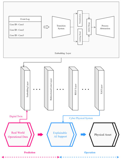
Figure 8. Smart factory manufacturing cooperative AI-workers framework.

3.2. Data Preprocessing

We used log data to predict manufacturing process time. All activities and machine names used in the manufacturing process are classified, and data were preprocessed using the transfer system method. Afterward, all data are vectorized so that they can be learned using an AI algorithm before learning. The specific deployment sequence of the model used in this paper can be seen in Figure 2. The event log data generated in the manufacturing process is preprocessed using the model and trained through the BI-LSTM Layer and the RELU Layer. Together with the learned results, it creates more visual results through only the XAI layer so that humans can better understand the operation of AI and that the system can have high reliability. The digital twin created by our model can help SMEs that find it difficult to adopt AI due to the lack of human resources, and by using explainable AI, it can also lead to collaboration between AI and workers working in real workspaces. Event logs generated in the manufacturing process are collected and tracked through IoT devices attached to machines used in each manufacturing process. In this paper, data preprocessing is performed based on the transition system, as described above, for the generated event log data, and normalization is performed based on the manufacturing QTY for AI learning.

Table 2 is the result of normalizing the data described in Table 1 based on QTY after preprocessing the data using the transition system. The trace column represents the manufacturing process time according to the process state confirmed according to the trace of Case ID. The regular part of the trace column explains which process the lot has passed, while the superscript of the process number means the time when the process started. Event log data includes the start time and end time according to each state, and the process start time is normalized to 0 according to Case ID. That is, in Table 1, the start time of 01-20-2022: 11:00 is mapped to 0, and the start time of Machine 2, 01-20-2022: 11:20 minus the start time, is 20. Case ID is process 2; it is the starting time. To put it more simply, this means that in Case ID 01, the second machine starts the process after 20 min, and all process end times in Case 01 can be interpreted as 100. The process sequence of Case 01 can be understood in more detail through Figure 9.

Table 2. Normalization of the event log.

Case ID	Trace	Product	Qtty	End Time
Case01	$<1^0,2^{20},3^{55},4^{80}>$	A	10	90
Case02	$<1^0,3^{40},2^{90},4^{140}>$	B	20	180
Case03	$<1^0,3^{32},2^{55},4^{90}>$	A	5	115
Case04	$<1^0,2^{42},3^{65},4^{210}>$	B	10	190
Case05	$<1^0,2^{35},??,??>$	B	10	$??$

Figure 9. Transition system.

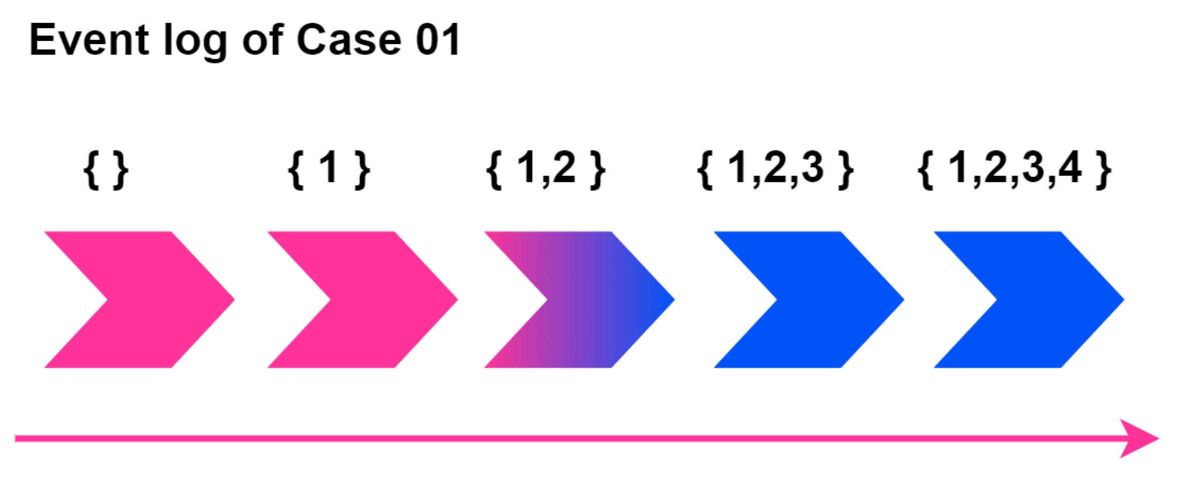
Figure 9 visually explains the mapping information according to the order in which Case 01 is traced, and the process that the lot has reached until the product is created. At this time, the tracked information is <1, 2, 3, 4>, along with process sequence information, and the type of machine used to manufacture the product can be checked. Each node in the figure means that the lot is tracked in the manufacturing process, and the number corresponding to the node is information that maps the manufacturing process and machine name that the lot passes through in the manufacturing line. More specifically, 1 state is a state of a product or component that has passed through manufacturing machine 1, while 1, 2, 3 state describes a state of a product or component that has passed through manufacturing machine 1, machine 2, and machine 3.

As described in Figure 8, this paper seeks to create a digital twin model that predicts the manufacturing process time by preprocessing the event log data accumulated in the manufacturing process. Vectorization was carried out to process data for learning AI. Table 3 shows the vectorized data of Case 01 in Table 2. Product means the product produced by Case 01, and each numeric column represents the manufacturing process, which means the machine name, while Remaining Time describes the remaining manufacturing process duration. At this time, each element of the vector is an integer indicating which processes have been tracked in the current state.

Table 3. Transformation of database.

Product	1	2	3	4	5	Execution Time
A	0	0	0	0	0	20.0
A	1	0	0	0	0	16.0
A	1	1	0	0	0	9.0
A	1	1	1	0	0	2.0

As described above, to normalize the QTY, which is the number of products produced, the End Time is subtracted from the traced value in Table 2, and the resultant is divided by the QTY manufactured in each Case ID. The formula used here is as follows:

$$\mathrm{Execution}\mathrm{Time}\left(S,P_{\mathrm{product}}\right)=\frac{S_{\mathrm{End}\mathrm{time}}-S_{\mathrm{Machine}\mathrm{start}\mathrm{time}}}{P_{\mathrm{product}}}$$

(12)

$$\begin{array}{cc}\hfill & \mathrm{Execution}\mathrm{Time}(<1>,5)=\frac{100-0}{5}=20.0\hfill \\ \hfill & \mathrm{Execution}\mathrm{Time}(<1,2>,5)=\frac{100-20}{5}=16.0\hfill \\ \hfill & \mathrm{Execution}\mathrm{Time}(<1,2,3>,5)=\frac{100-55}{5}=9.0\hfill \\ \hfill & \mathrm{Execution}\mathrm{Time}(<1,2,3,4>,5)=\frac{100-90}{5}=2.0\hfill \end{array}$$

(13)

This paper performs the data preprocessing specifically described in this section for manufacturing process prediction. After the next process, the remaining process time is used as a Y vector of deep learning, and an integer matrix indicating whether each machine is executed or not is used as an X vector for learning. The following section describes the XAI model used in this study.

3.3. XAI Procedures

The model proposed in this paper is based on regression analysis. To evaluate the results obtained through regression analysis, the mean absolute error (MAE) is used as a performance indicator of the learning model. We also use the Bi-LSTM model, which shows excellent ability to learn ordered data. The model presented in this paper uses log data, as shown in the figure, and firstly performs data preprocessing using a transition system. After that, it learns in the Bi-LSTM layer. Finally, the generated model is passed through the SHAP XAI layer to create a visual graph that can be interpreted by humans. SHAP is a model that helps humans find the causative factors of complex neural network model results that cannot be understood by humans, based on the Shapley value and how much it affects the results [32]. The first thing a human needs to know about SHAP is the Shapley values.

Figure 10 is a schematic showing the flow chart of the SHAP operation. In general, neural network models predict results through complex operations in a process called black-box. However, as it is called black-box, it is not known how the predictive model derived the result. However, XAI (Explainable-AI)-like SHAP expresses the reason why the predictive model derives these results as a Shapley value by analyzing the black box model using the surrogate model [33]. In general, the predictive model is expressed as f, and the explanatory model to explain the predictive model is expressed as g. Finally, SHAP is used to find a Surrogate Model $\left(g\right)$ that satisfies the following formula by putting $x^{\prime }$, which will satisfy $x=h_x\left(x^{\prime }\right)$, as an input value, not the same value as the input value for the prediction model.

$$g\left(z^{\prime }\right)=f\left(h_x\left(z^{\prime }\right)\right)where{z}^{\prime }\approx x^{\prime }$$

(14)

$$g\left(z^{\prime }\right)={\varphi }_0+\sum _{t=1}^M{\varphi }_t{z}_t^{\prime }$$

(15)

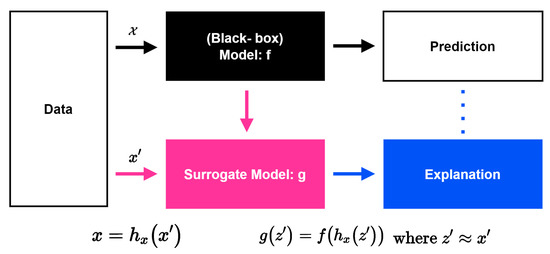
Figure 10. SHAP flow chart.

M is the number of simplified input values to enter the surrogate model, and $z^{\prime }$ represents a vector of binary variables of size M. Each feature satisfies ${\varphi }_t\in R$.

Next, we will examine the Shapley value, which plays the most important role in SHAP explaining the prediction model. As shown in the above formula, the effect value can be obtained based on game theory. Furthermore, the Shapley value can be found based on ‘game theory’ for fair game defined by Lloyd Shapley. The game theory proposed by Lloyd Shapley must satisfy the following four conditions, which means the rules for calculating the total amount earned by all players.

(1)

The total reward should be equal to the sum of the rewards received by everyone.

(2)

If both players contribute the same value, they must also receive the same reward.

(3)

No value contribution means that you will not receive any compensation.

(4)

When playing two games, the total reward for each individual must be equal to the sum of the rewards from the first game and the rewards from the second game.

The above four conditions are similar to the conditions required to estimate the Shapley value. Using the condition proposed by Lloyd Shapley, the following three characteristics of Shapley value can be known:

• First condition (Local accuracy)

  $$f\left(x\right)=g\left(x^{\prime }\right)={\varphi }_0+\sum _{t=1}^M{\varphi }_i{x}_t^{\prime }$$

  (16)
  When the Surrogate model $g\left(x^{\prime }\right)$ is $x=h_{-}x\left(x^{\prime }\right)$, it shows that it is the same as the predictive model $f\left(x\right)$.
• Second condition (Missingness)

  $$x_t^{\prime }=0\to {\varphi }_t=0$$

  (17)
  If there is no feature in the existing input value, it has no effect.
• Third condition (Consistency)

  $$f^{\prime }\left(h_x\left(z^{\prime }\right)\right)-f^{\prime }\left(h_x\left(z_t^{\prime }=0\right)\right)\ge f\left(h_x\left(z^{\prime }\right)\right)-f\left({\mathrm{h}}_x\left(z_t^{\prime }=0\right)\right),\forall z^{\prime }{\{0,1\}}^M,$$

  (18)

  $$\mathrm{then}{\varphi }_t\left(f^{\prime },x\right)\ge {\varphi }_t(f,x)$$

  (19)
  The above formula shows that if the model is changed and the contribution of the simplified input value increases, the input’s attribution should not decrease. In conclusion, the explainable model g satisfies $g\left(z^{\prime }\right)=f\left(h_x\left(z^{\prime }\right)\right)$ where $z^{\prime }\approx x^{\prime }$ and must satisfy all three conditions above.

  $${\varphi }_t(f,x)=\sum _{z^{\prime }\subseteq x^{\prime }}\frac{\left|z^{\prime }\right|!\left(M-\left|z^{\prime }\right|-1\right)!}{M!}\left[f\left(h_x\left(z^{\prime }\right)\right)-f\left(h_x\left(z_t^{\prime }=0\right)\right)\right]$$

  (20)

If the above three conditions are satisfied, the SHAP value can be obtained, as shown in the above formula. Each value means how much the size of the output is changed, where $\left|z^{\prime }\right|$ means the number of non-zero values among the values of $Z^{\prime }$, and $Z^{\prime }\subseteq x^{\prime }$ means that all $Z^{\prime }$ vectors are zero. It means that it is a subset of $X^{\prime }$ values.

Figure 11 is a visualization image of how the Shapley value explains the prediction model. According to the figure above, the longer the length of the arrow, the greater the influence the corresponding feature had on the result. Features that increase the result function value are marked with a right arrow in red, while features that decrease the result value are marked with a left arrow in blue. In conclusion, through the length and direction of the arrow, it is possible to visually check the features that have a major influence on the results of the prediction model. If this characteristic of SHAP is applied to a model trained on manufacturing data, process workers can discover features that have a major impact on prediction results in the manufacturing process. It can also have a positive impact on sophisticated modifications of predictive models.

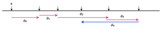
Figure 11. Visualization of SHAP results.

4. Performance Analysis

4.1. Metalworking Process Data Set and Evaluation Indicators

This paper used event log data of the metal processing process. As in the Table 4, the data set includes information about the machining process, such as Case ID, Activity, Start Time, Complete Time, and Resource. Reference [34] implemented an event prediction model through LSTM neural network implementation using the data set and predicted the time until the next activity. The metal processing process consists of activities such as grinding, turning, and lapping, and the data set can be checked in more detail through the table. Case 9 of the metal processing process data set will be described in a table. The data are more simply written in the activity of the name of the process used in the actual manufacturing process, and each case produces a product through the operation of 28 machines. In this paper, the data of each case are preprocessed based on the transition system, and as described above, through the vectorization process, it is produced in the form of data that AI can learn. The BI-LSTM algorithm is then used to create a digital twin model that predicts the manufacturing process time. A graph that can be visually interpreted together with the prediction results is generated to make the AI model into an explainable AI in a form that can be interpreted by humans so that the results predicted by the model can be immediately applied to the physical asset through the CPS. In this paper, to create a more meaningful digital twin model, we proceeded with the abstraction process of the iterative process. For highly complex manufacturing processes, this may not be suitable for AI neural network training, and for repetitive activities, it may interfere with the understanding of the process [35]. We used the mean absolute error (MAE) as an evaluation index of the model to prove the performance of the AI model in predicting the manufacturing process time using the transition system-based data preprocessing method.

$$\mathrm{MAE}=\frac{1}{n}\sum _{t=1}^n\left|A_t-F_t\right|$$

(21)

Table 4. Metal processing event log of Case 9.

Case ID	Activity Machine	Start Time	Complete Time	Qty
Case 9	Turning—Machine 9	2012-01-30    14:38	2012-01-30   15:59	20
Case 9	Turning—Machine 9	2012-01-30   16:07	2012-01-30   17:34	20
Case 9	Turning—Machine 9	2012-01-30   17:35	2012-01-30   21:03	20
Case 9	Turning Q.C.	2012-02-01   07:23	2012-02-01   07:30	20
Case 9	Lapping—Machine 1	2012-02-01   09:54	2012-02-01   11:18	20
Case 9	Lapping—Machine 1	2012-02-14   15:13	2012-02-14   17:18	20
Case 9	Round Grinding—Manual	2012-02-16   06:58	2012-02-16   08:09	20
Case 9	Round Grinding—Manual	2012-02-16   08:09	2012-02-16   11:11	20
Case 9	Laser Marking—Machine 7	2012-02-16   11:29	2012-02-16   11:30	20
Case 9	Final Inspection Q.C.	2012-02-19   13:20	2012-02-19   15:00	20
Case 9	Final Inspection Q.C.	2012-02-20   09:07	2012-02-20   09:08	20
Case 9	Packing	2012-02-21   00:00	2012-02-21   01:00	20

In addition, through SHAP, the AI model learned using the data preprocessing method proposed in this paper can be visualized, and the operation method of the model can be interpreted.

4.2. Hyperparameter

As can be seen from the Table 5 in this study, Intel core i7 was used for the CPU, the RAM was configured with 64 GB, and the GeForce 1660TI was used for the graphics card. In addition, we implemented deep learning using the Keras Python library in the experiment and used the SHAP library to implement SHAP values. Hyperparameter values were as follows. Epochs were fixed at 1000 times, and the early stop function was not used. The batch size was fixed at 40, and the optimizer was used by customizing AdaGrad. In addition, the unit of BI-LSTM was set to 128 to learn data.

Table 5. Description of Parameters.

Parameter	Description
CPU	Intel core i7
Ram	64 GB
Graphics Card	Geforce 1660TI

4.3. Model Evaluation

This section quantitatively explains that the model learning method proposed in this paper can produce meaningful results in the manufacturing process. We used two algorithms for AI learning. First, the model was trained LSTM, and the hidden characteristics of data were reflected using Bi-LSTM with a reverse LSTM layer added. As described above, the data set used for this experiment is a metal processing process data set, and each feature is a combination of the machine model name and function used for the manufacturing process. As a hyperparameter in this experiment, batch size was set to 40. Epochs were unified as 1000, and the learning rate was set to 0.001. MAE was used as an evaluation index, and as a result of the experiment, both the LSTM model and the Bi-LSTM model were able to obtain positive results as the number of learning increased and showed convergence when a specific epoch was exceeded. In addition, a comparison of the results of the model using the validation set and the model using the train set shows that there is no overfitting to one side, indicating that the learning results of the corresponding model are significant. The LSTM model converges to 0.45 (hour), and when the Bi-LSTM algorithm is used, the LSTM model converges to 0.15 (hour).

Figure 12 is the result of training using the LSTM algorithm to predict the manufacturing process time. As the epoch increases, they all move downwards to the right. The graph on the left shows the results of the Train Model, while the graph on the right shows the results of the Test Model. When the two models are compared, they can be checked for not being overfitted, such as biased to one side; this validates the corresponding model. In the case of the model using the LSTM algorithm, it is evident that the MAE decreases rapidly up to 200 epochs, and the lowest MAE value is 0.45 (hour), which converges at the 0.45 level through the graph.

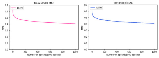
Figure 12. Comparison between train data and test data of the model using the LSTM algorithm.

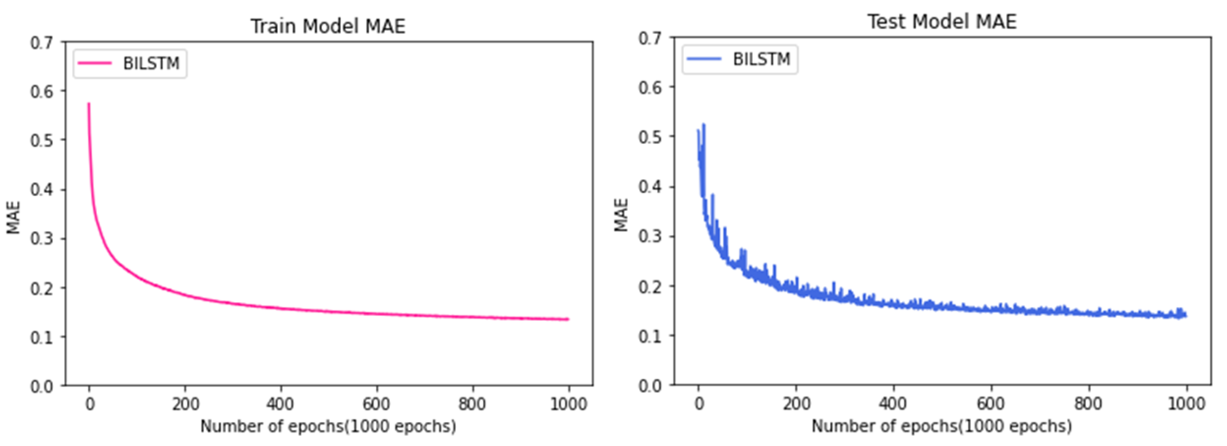
Figure 13 is the result of learning to predict the manufacturing process time using the BI-LSTM algorithm, as shown in the previous figure. Both the Train Model and the Test Model showed a downward trend and showed convergence after a certain epoch. Furthermore, a comparison of the two graphs shows that the learning was properly accomplished through the fact that overfitting, such as biasing, did not occur. The Test Model graph shows that it gradually converges from 150 to 200 Epoch, and the best result was 0.15 (hour).

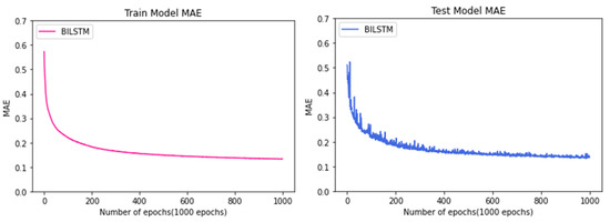
Figure 13. Comparison between train data and test data of the model using the BI-LSTM algorithm.

4.4. Model Comparison

In this experiment, we used and compared the LSTM algorithm and the BI-LSTM algorithm using data obtained from the metal processing process and additionally tried XAI using the SHAP value.

4.4.1. Comparative Analysis

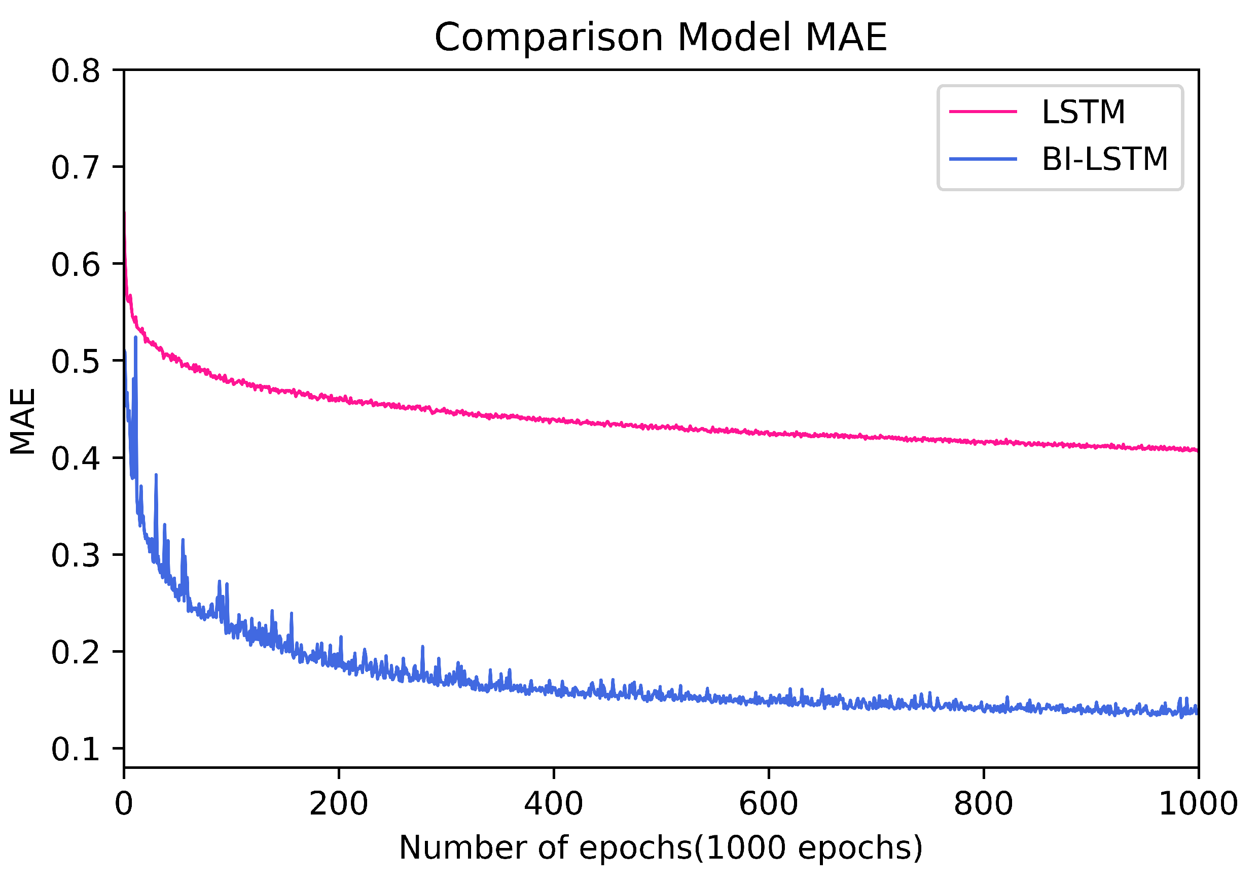
Algorithm learning was conducted in the Geforce 1660TI environment, as described above, and Figure 14 below is a graph comparing the LSTM and BI-LSTM learning results. In batch size 40, the execution time for each epoch was less than 10 s, and the same training was performed with 1000 epochs.

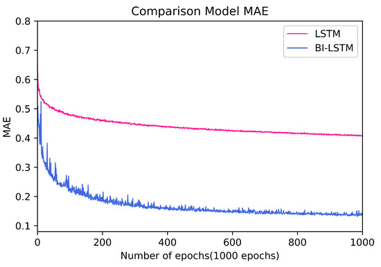
Figure 14. Comparison of the training model.

As a result of learning, BI-LSTM obtained relatively superior results compared to LSTM. Both LSTM and BI-LSTM showed convergence around 200 epochs, but the MAE of the model learned through BI-LSTM obtained better results than LSTM. In the case of the LSTM model, it converges to 0.45 after 200 epochs, and in the case of BI-LSTM, it can be confirmed through the graph that it converges to 0.15 after 200 epochs. In terms of convergence speed, both algorithms obtained similar results, but BI-LSTM obtained an excellent result, about 2.5 times greater than the learning result of LSTM provided. Although there is no significant difference in learning speed between the two models, the figure shows that BI-LSTM is effective in predicting manufacturing process time. In addition, we proved that this paper can obtain meaningful results through comparative results.

4.4.2. SHAP Values and Prediction

The idea of the Shapley value was derived from game theory, as described above. This paper was used to interpret the prediction results of the proposed AI model using the Shapley value, and positive results were obtained to induce collaboration between workers and AI. The model proposed in this paper preprocesses the event log data using a transition system and predicts the manufacturing process time by learning the data. Features can affect the results predicted by the model. The data we used is from the metal processing process of the real world, and the features of the data learned by the AI in this paper refer to several manufacturing machines in the manufacturing process. The contribution of these features is called the SHAP value. That is, since the Y vector in this paper is the remaining time of the manufacturing process, the degree of influence that each manufacturing machine has on the manufacturing process can be known through the SHAP value.

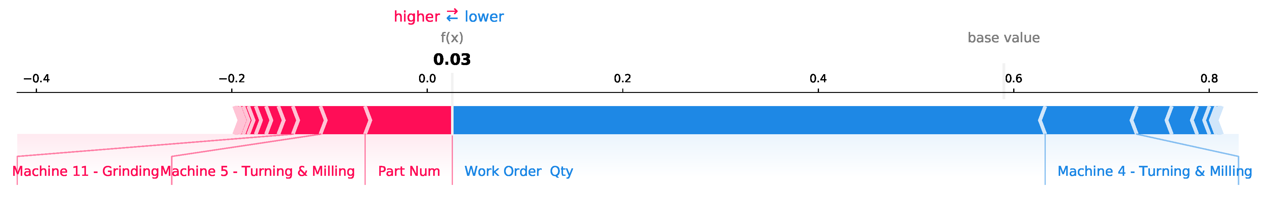
The data learned in this paper is a metal processing process, and Figure 15 shows the SHAP value of one of the cases that produce a cable head. The red arrow in the figure indicates the factors that affect the increase in the prediction result value, while in contrast, the blue arrow explains the factors that affect the decrease in the prediction result value. The length of the arrow quantitatively expresses the extent to which the corresponding feature contributed to the prediction result and corresponds to the SHAP value. Because the result that this model learned and predicted is the remaining time of the manufacturing process, Machine 11—Grinding, Machine 5—Turning and Milling had an impact on increasing the manufacturing process time, and Work Order Qty, Machine 4—Turning and Milling. It had the effect of reducing the manufacturing process time. Part Num was excluded from the analysis of XAI because it is a number used to classify manufactured products.

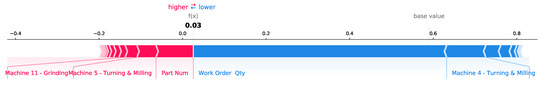
Figure 15. SHAP values of cable head.

Figure 16 shows the SHAP value of one of the cases producing spur gear generated in the metal manufacturing process. As described above, the red arrow in the figure shows the features that have an effect on increasing the manufacturing process time, while the blue arrow shows the features that have an effect on reducing the manufacturing process time. The length of the arrow is a quantitative expression of the degree of contribution and means a relative value for the case that is being described. Through the figure, we show that Packing, Machine 10—-Grinding had a positive effect on increasing the manufacturing process time, and Work Order Qty, Quality Check 1 had a positive effect on reducing the manufacturing process time in the case of generating Spur Gear. The Part Num of the graph was also excluded from the analysis of XAI because it is a random number to distinguish the manufactured products.

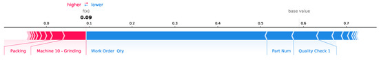
Figure 16. SHAP values of Spur Gear.

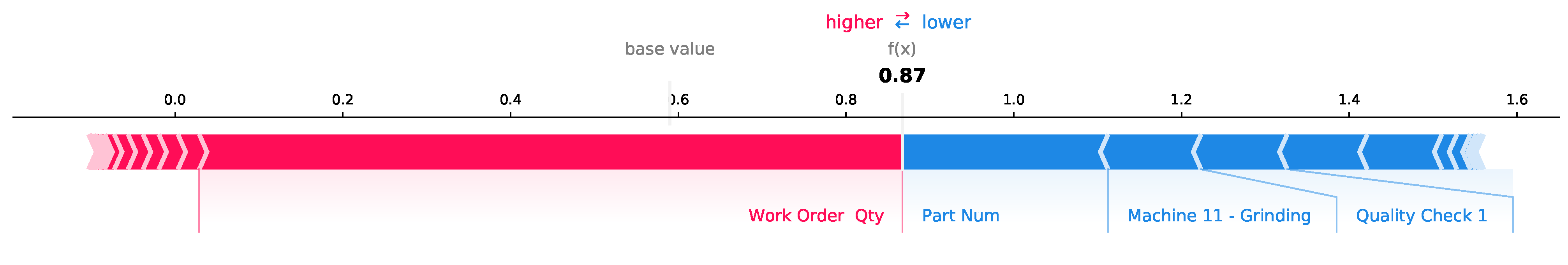
Figure 17 explains the SHAP value of one of the cases producing Ball Nuts. In this case, Work Order Qty had a significant effect on delaying the manufacturing process time, while Machine 11—Grinding and Quailty Check1 had an effect on shortening the manufacturing time. Likewise, Part Num was excluded from the analysis because it is a number mapped to distinguish production products. With the local accuracy property of the SHAP value, it is possible to provide a meaningful estimate of the contribution of the feature to the variation in the predicted time of the manufacturing process time of the case. In addition, the estimate can help field experts in the manufacturing process determine the appropriateness of direct learning without interpretation by AI experts and provide an appropriate indicator to increase the accuracy of AI models. Furthermore, AI directly grasps the manufacturing environment through manufacturing process data, adjusts the manufacturing process by self-judgment without the intervention of a consultant, and builds an automatic system that provides the operator with the reason for modifying the manufacturing process through an intuitive graph. We believe that such research can have a positive impact.

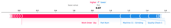
Figure 17. SHAP values of Ball Nuts.

This paper tried to explain the AI that predicts the manufacturing process time more visually by using the characteristics of the SHAP value. As a result, this paper has achieved positive results in explaining how AI works to manufacturing process workers in the real world through graphs.

5. Conclusions

In this paper, log data were traced to predict the manufacturing process time, and data preprocessing was performed based on the transition system. In addition, learning was carried out using the Bi-LSTM, but LSTM has a disadvantage in that it tends to converge based on the previous pattern. To improve the performance of the LSTM, a BI-LSTM with the addition of a reverse LSTM has been developed. This paper tried to predict the manufacturing execution time, and it was proved through experiments that better results can be obtained when bidirectional learning is performed than when prediction is performed based on only previous manufacturing execution information. In this paper, when directly comparing the experimental results of BI-LSTM and LSTM, BI-LSTM gradually converged between 150 and 200 epochs, and 0.15 (Hour) was obtained as the best MAE result. This result showed that it was about 2.5 times larger than the experimental result of LSTM, 0.45 (Hour), to obtain an excellent result. In addition, we tried to explain AI through SHAP, and we tried to prove that the method is valid. As far as we know, it is the first attempt to make an AI learning process time prediction model based on a transition system into an explainable model. To prove that our method is valid, an AI model was formed using various algorithms, and the experimental results were compared and analyzed. In addition, we tried to change the generated model into an XAI model, and a qualitative analysis was made possible through a visual graph. The results of the experiments performed in this paper show the possibility of changing the manufacturing process prediction model trained based on the transition system into an explanatory AI model. According to the rapidly changing consumption trend in Industry 4.0, the manufacturing environment becomes more complex, and requires flexibility to change rapidly according to the environment. Therefore, now that the traditional method of changing process operations based on the experience of consultants or experts is changing to the method of using an AI model that has learned big data, the black box characteristic that cannot explain how AI works is manufacturing AI. This causes the biggest problem in using it in the process. The transition system-based explanatory AI model proposed in this paper can help SMEs with insufficient human resources apply the CPS that creates the best operating results in real-time according to the manufacturing process environment. Partners using the technology in this paper can gain valuable insights to further advance their manufacturing processes through the insights provided by XAI. In this paper, the BI-LSTM model is used to predict the manufacturing process time. Afterward, we will upgrade the model to develop better results in the thesis, and although we conducted our research in the manufacturing industry, we consider that it can be conducted in other industries as well and that it is a necessary research topic in other industries.

References

- Lee, C.H.; Liu, C.L.; Trappey, A.J.; Mo, J.P.; Desouza, K.C. Understanding digital transformation in advanced manufacturing and engineering: A bibliometric analysis, topic modeling and research trend discovery. Adv. Eng. Inform. 2021, 50, 101428. [Google Scholar] [CrossRef]
- Trappey, A.J.; Trappey, C.V.; Govindarajan, U.H.; Sun, J.J.; Chuang, A.C. A review of technology standards and patent portfolios for enabling cyber-physical systems in advanced manufacturing. IEEE Access 2016, 4, 7356–7382. [Google Scholar] [CrossRef]
- Zheng, T.; Ardolino, M.; Bacchetti, A.; Perona, M. The applications of Industry 4.0 technologies in manufacturing context: A systematic literature review. Int. J. Prod. Res. 2021, 59, 1922–1954. [Google Scholar] [CrossRef]
- Zheng, P.; Sivabalan, A.S. A generic tri-model-based approach for product-level digital twin development in a smart manufacturing environment. Robot. -Comput.-Integr. Manuf. 2020, 64, 101958. [Google Scholar] [CrossRef]
- Rasheed, A.; San, O.; Kvamsdal, T. Digital twin: Values, challenges and enablers from a modeling perspective. IEEE Access 2020, 8, 21980–22012. [Google Scholar] [CrossRef]
- Mehdiyev, N.; Evermann, J.; Fettke, P. A novel business process prediction model using a deep learning method. Bus. Inf. Syst. Eng. 2020, 62, 143–157. [Google Scholar] [CrossRef] [Green Version]
- Chien, C.H.; Chen, P.Y.; Trappey, A.J.; Trappey, C.V. Intelligent Supply Chain Management Modules Enabling Advanced Manufacturing for the Electric-Mechanical Equipment Industry. Complexity 2022, 2022, 8221706. [Google Scholar] [CrossRef]
- Wang, C.C.; Chien, C.H.; Trappey, A.J. On the application of ARIMA and LSTM to predict order demand based on short lead time and on-time delivery requirements. Processes 2021, 9, 1157. [Google Scholar] [CrossRef]
- Thoppil, N.M.; Vasu, V.; Rao, C. Bayesian optimization LSTM/bi-LSTM network with self-optimized structure and hyperparameters for remaining useful life estimation of lathe spindle unit. J. Comput. Inf. Sci. Eng. 2022, 22, 021012. [Google Scholar] [CrossRef]
- Habbouche, H.; Benkedjouh, T.; Zerhouni, N. Intelligent prognostics of bearings based on bidirectional long short-term memory and wavelet packet decomposition. Int. J. Adv. Manuf. Technol. 2021, 114, 145–157. [Google Scholar] [CrossRef]
- Yang, M.; Moon, J.; Jeong, J.; Sin, S.; Kim, J. A Novel Embedding Model Based on a Transition System for Building Industry-Collaborative Digital Twin. Appl. Sci. 2022, 12, 553. [Google Scholar] [CrossRef]
- Lu, Y.; Liu, C.; Kevin, I.; Wang, K.; Huang, H.; Xu, X. Digital Twin-driven smart manufacturing: Connotation, reference model, applications and research issues. Robot. Comput.-Integr. Manuf. 2020, 61, 101837. [Google Scholar] [CrossRef]
- Tao, F.; Qi, Q.; Liu, A.; Kusiak, A. Data-driven smart manufacturing. J. Manuf. Syst. 2018, 48, 157–169. [Google Scholar] [CrossRef]
- Zhang, C.; Chen, D.; Tao, F.; Liu, A. Data driven smart customization. Procedia CIRP 2019, 81, 564–569. [Google Scholar] [CrossRef]
- Leitão, P.; Colombo, A.W.; Karnouskos, S. Industrial automation based on cyber-physical systems technologies: Prototype implementations and challenges. Comput. Ind. 2016, 81, 11–25. [Google Scholar] [CrossRef] [Green Version]
- Lu, Y.; Asghar, M.R. Semantic communications between distributed cyber-physical systems towards collaborative automation for smart manufacturing. J. Manuf. Syst. 2020, 55, 348–359. [Google Scholar] [CrossRef]
- Groshev, M.; Guimarães, C.; Martín-Pérez, J.; de la Oliva, A. Toward intelligent cyber-physical systems: Digital twin meets artificial intelligence. IEEE Commun. Mag. 2021, 59, 14–20. [Google Scholar] [CrossRef]
- Ghahramani, M.; Qiao, Y.; Zhou, M.; Hagan, A.O.; Sweeney, J. AI-based modeling and data-driven evaluation for smart manufacturing processes. IEEE/CAA J. Autom. Sin. 2020, 7, 1026–1037. [Google Scholar] [CrossRef]
- Ding, H.; Gao, R.X.; Isaksson, A.J.; Landers, R.G.; Parisini, T.; Yuan, Y. State of AI-based monitoring in smart manufacturing and introduction to focused section. IEEE/ASME Trans. Mechatron. 2020, 25, 2143–2154. [Google Scholar] [CrossRef]
- Noto La Diega, G.; Walden, I. Contracting for the ‘Internet of Things’: Looking into the Nest. Queen Mary School of Law Legal Studies Research Paper No. 219/2016. Available online: https://ssrn.com/abstract=2725913 (accessed on 21 June 2022).
- Shafique, K.; Khawaja, B.A.; Sabir, F.; Qazi, S.; Mustaqim, M. Internet of things (IoT) for next-generation smart systems: A review of current challenges, future trends and prospects for emerging 5G-IoT scenarios. IEEE Access 2020, 8, 23022–23040. [Google Scholar] [CrossRef]
- Montavon, G.; Samek, W.; Müller, K.R. Methods for interpreting and understanding deep neural networks. Digit. Signal Process. 2018, 73, 1–15. [Google Scholar] [CrossRef]
- Arrieta, A.B.; Díaz-Rodríguez, N.; Del Ser, J.; Bennetot, A.; Tabik, S.; Barbado, A.; García, S.; Gil-López, S.; Molina, D.; Benjamins, R.; et al. Explainable Artificial Intelligence (XAI): Concepts, taxonomies, opportunities and challenges toward responsible AI. Inf. Fusion 2020, 58, 82–115. [Google Scholar] [CrossRef] [Green Version]
- Dave, D.; Naik, H.; Singhal, S.; Patel, P. Explainable ai meets healthcare: A study on heart disease dataset. arXiv 2020, arXiv:2011.03195. [Google Scholar]
- Ribeiro, M.T.; Singh, S.; Guestrin, C. “Why should i trust you?” Explaining the predictions of any classifier. In Proceedings of the 22nd ACM SIGKDD International Conference on Knowledge Discovery and Data Mining, San Francisco, CA, USA, 13–17 August 2016; pp. 1135–1144. [Google Scholar]
- van der Aalst, W.M. Process mining and simulation: A match made in heaven! In Proceedings of the SummerSim, Bordeaux, France, 9–12 July 2018; pp. 4:1–4:12. [Google Scholar]
- Bergmann, S.; Feldkamp, N.; Strassburger, S. Approximation of dispatching rules for manufacturing simulation using data mining methods. In Proceedings of the 2015 Winter Simulation Conference (WSC), Huntington Beach, CA, USA, 6–9 December 2015; pp. 2329–2340. [Google Scholar]
- Kusiak, A. Smart manufacturing must embrace big data. Nature 2017, 544, 7648. [Google Scholar] [CrossRef] [PubMed]
- Lugaresi, G.; Zanotti, M.; Tarasconi, D.; Matta, A. Manufacturing Systems Mining: Generation of Real-Time Discrete Event Simulation Models. In Proceedings of the 2019 IEEE International Conference on Systems, Man and Cybernetics (SMC), Bari, Italy, 6–9 October 2019; pp. 415–420. [Google Scholar]
- Rahman, M.; Watanobe, Y.; Nakamura, K. A neural network based intelligent support model for program code completion. Sci. Program. 2020, 2020, 7426461. [Google Scholar] [CrossRef]
- Rahman, M.; Watanobe, Y.; Nakamura, K. A bidirectional LSTM language model for code evaluation and repair. Symmetry 2021, 13, 247. [Google Scholar] [CrossRef]
- Myklebust, I.O. Explainable AI Methods for Cyber-Physical Systems. Master’s Thesis, National Taiwan Normal University, Taipei, Taiwan, 2021. [Google Scholar]
- Lundberg, S.M.; Erion, G.; Chen, H.; DeGrave, A.; Prutkin, J.M.; Nair, B.; Katz, R.; Himmelfarb, J.; Bansal, N.; Lee, S.I. From local explanations to global understanding with explainable AI for trees. Nat. Mach. Intell. 2020, 2, 56–67. [Google Scholar] [CrossRef]
- Tello-Leal, E.; Roa, J.; Rubiolo, M.; Ramirez-Alcocer, U.M. Predicting activities in business processes with LSTM recurrent neural networks. In Proceedings of the 2018 ITU Kaleidoscope: Machine Learning for a 5G Future (ITU K), Santa Fe, Argentina, 26–28 November 2018; pp. 1–7. [Google Scholar]
- Lugaresi, G.; Matta, A. Automated manufacturing system discovery and digital twin generation. J. Manuf. Syst. 2021, 59, 51–66. [Google Scholar] [CrossRef]
Publisher’s Note: MDPI stays neutral with regard to jurisdictional claims in published maps and institutional affiliations. |
© 2022 by the authors. Licensee MDPI, Basel, Switzerland. This article is an open access article distributed under the terms and conditions of the Creative Commons Attribution (CC BY) license (https://creativecommons.org/licenses/by/4.0/).