Abstract
This work involves a heuristic for solving vehicle routing problems with time windows (VRPTW) with general compatibility-matching between customer/patient and server/caretaker constraints to capture the nature of systems such as caretakers’ home visiting systems or home healthcare (HHC) systems. Since any variation of VRPTW is more complicated than regular VRP, a specific, custom-made heuristic is needed to solve the problem. The heuristic proposed in this work is an efficient hybrid of a novice Local Search (LS), Ruin and Recreate procedure (R&R) and Particle Swarm Optimization (PSO). The proposed LS acts as the initial solution finder as well as the engine for finding a feasible/local optimum. While PSO helps in moving from current best solution to the next best solution, the R&R part allows the solution to be over-optimized and LS moves the solution back on the feasible side. To test our heuristic, we solved 56 benchmark instances of 25, 50, and 100 customers and found that our heuristics can find 52, 21, and 18 optimal cases, respectively. To further investigate the proficiency of our heuristic, we modified the benchmark instances to include compatibility constraints. The results show that our heuristic can reach the optimal solutions in 5 out of 56 instances.
1. Introduction
In the year 2020, the proportion of the Thai population aged over 65 was 19.8%, more than double the global average of 9.3%. This figure is expected to increase to 29.6% over the next 30 years [1]. This means that in a short period of time Thailand will become a Super Aged country, defined as a country where more than 28% of the population is over 60 years of age. As projected by the Office of the National Economic and Social Development Board, Office of the Prime Minister, Bangkok, Thailand [2], the number of elderly people living alone with health problems will also increase. Home healthcare (HHC), which plays a major role in a proactive healthcare system, is essential for this population group, especially those with chronic diseases and bedridden patients requiring long-term care [3]. Caring for these people may involve injections, wound dressing, physical therapy, and other rehabilitation procedures, as well as health-related advice-giving to ensure the sustainability and improved life quality of the coming Aged Society. For the elderly, home visits represent more efficient management of human resources than having them visit the hospital individually.
In attempting to manage home visits in an HHC system, the following need to be considered: (1) compatibility matching of patients/customers and physicians, experts, or healthcare staff; (2) best routing for healthcare personnel to visit their customers; (3) meeting applicable service conditions, and (4) minimizing the cost of the whole system. The second consideration together with the fourth bear similarities to a regular VRP, and if the third is also considered, the problem becomes a vehicle routing problem with time windows (VRPTW). In this work, we will also integrate the first aspect into the VRPTW to better capture the nature of the HHC system. When all these aspects are taken into consideration, the problem becomes even more complicated and requires a custom-made heuristic to find a solution.
Most of the VRPTWs showcased in the literature already consider minimizing distance traveled as the main objective. The model we constructed can also deal with minimizing the total cost, with main objectives ranging from total distance traveled to completion time. This, along with the new general set of compatibility constraints, will make it more relevant for real-world applications, as patient-caretaker compatibility matching is sometimes necessary and minimizing waiting time and balancing job numbers per vehicle are a more important issue in VRPTWs that are similar to HHC systems.
The work process in this study goes as follows: First, a VRPTW with compatibility matching constraints is formulated. Subsequently, a hybrid heuristic combining local search (LS), Ruin and Recreate procedure (R&R), and particle swarm optimization (PSO) is proposed for solving the problem, which is NP-hard in nature. Finally, simulation results tested on best known benchmark instances, namely Solomon’s instances, are presented to show our heuristic’s efficiency in solving VRPTW problems with and without compatibility matching constraints.
This paper is organized as follows: Section 2 provides a review of literature on VRPTW. Section 3 presents a mathematical formulation of the problem. Section 4 describes the solution approach. Computational experiments on Solomon’s instances and conclusions are presented in Section 5 and Section 6, respectively.
2. Materials and Methods
As mentioned earlier, managing home visits in HHC systems can be viewed as a variety of VRPTW. In addition to minimizing the arrival time, finishing time, or processing time in caretaker-customer matching, the models may require further constraints to better suit the problems. Some existing works consider the travel cost, penalty cost, fixed cost, and overtime cost of the healthcare worker in their objective function. Wirnitzer et al. [4] find the minimum staff numbers including minimum number per hour and per customer and the number of staff replacing/switching times per customer. Braekers et al. [5] minimize the weighted sum costs while maximizing service level; therefore, the costs considered comprise the total costs and penalty costs that arise when customers find it inconvenient to receive service. Putting compatibility in the objective function, Ait Haddadene et al. [6] minimize total travel time as well as non-preferences between caretakers and patients to maximize compatibility while adding synchronization constraints, as some patients may need multiple services at the same time. Polnik et al. [7], also with synchronized visits to a home, construct a heuristic to solve the problem where each stop has only one task that might need multiple caretakers. Considering compatibility in the constraints, Yu et al. [8] minimize maximum traveling time with the vehicle allowed to visit only compatible nodes. Riazi et al. [9] consider minimizing total distance traveled but with caretaker qualification requirements in the constraints. In another work, Kandakoglu et al. [10] consider the weighted sum of total distance traveled, total travel cost, overtime wages and number of working staff; their notable constraints include the lunch break of the nurses. Nasir and Kuo [11] only consider the minimum total travel cost of staff but have synchronization constraints between nurses and vehicles as they consider the travel costs of the two separately. Cissé et al. [12] and Mascolo et al. [13] give the most recent extended review of literature in HHC routing and scheduling problems with variety of constraints to date.
Of the recently proposed heuristics for solving VRPTW that are more complicated than an NP-hard VRP, most are metaheuristics. The benchmark instances given in [14], known as Solomon’s instances, can be used to assess constructed heuristics. Table 1 shows the objective function values studied in the most recent literature. Note that only works that consider hard time windows, i.e., where the service providers need to wait for customers to become available, are presented in the table.

Table 1.
The best objective function values obtained in literature on Solomon’s instances.
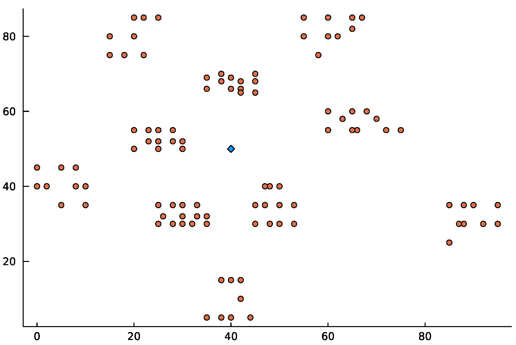
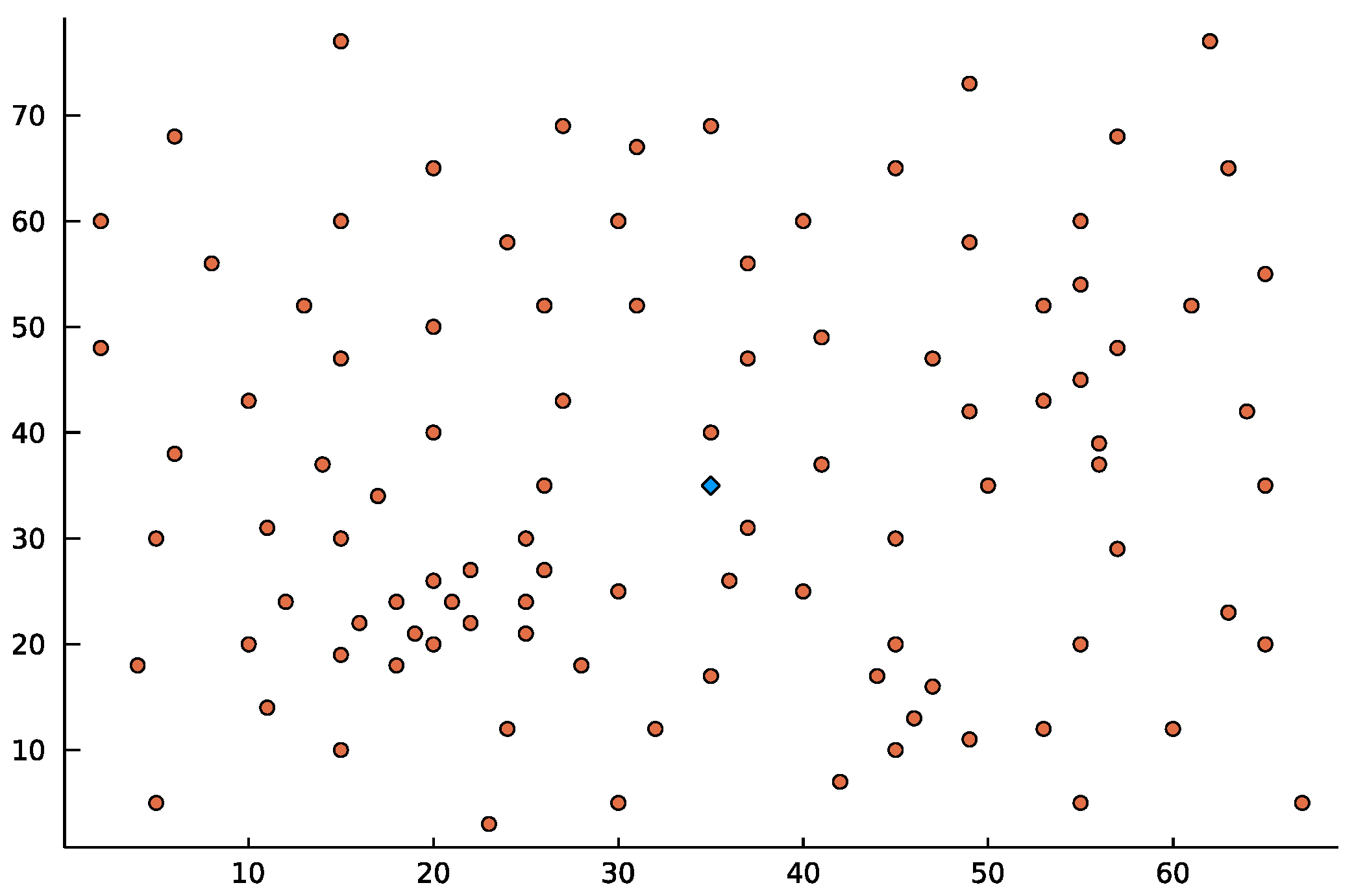
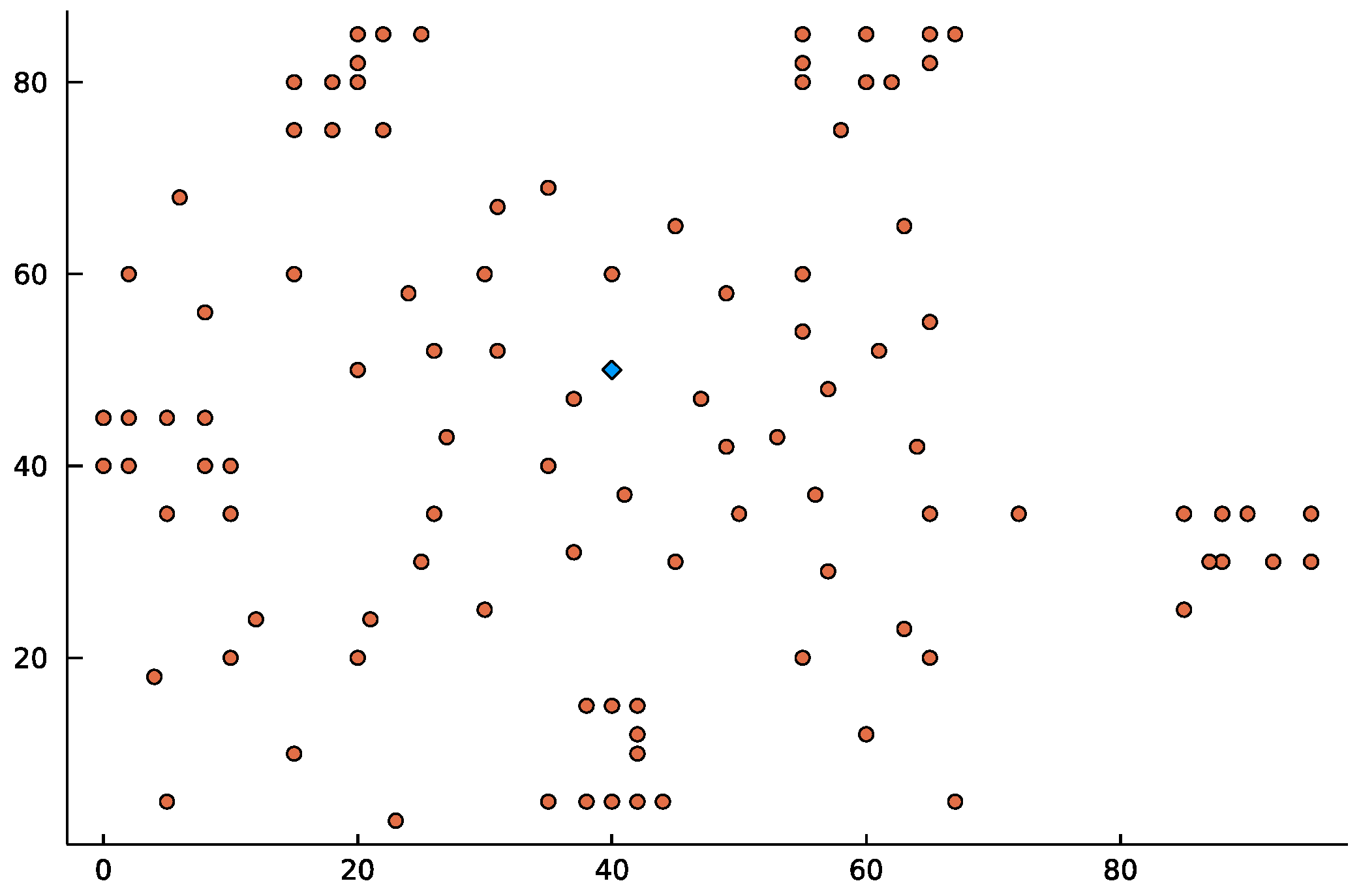
There are three groups of Solomon’s instances. After plotting these instances, we can see that the customers in Group C instances appear to be scattered in groups or clusters, as seen in Figure 1. These instances are similar to real-world problems where customers live in geographically scattered villages. The customers in Group R instances (Figure 2) are relatively randomly placed, corresponding to customers living in a big city. The customers in Group RC (Figure 3) are randomly clustered, that is, they appear in groups, but within these groups, they are more or less randomly placed. This system can also be found in a typical real-world system as well. Since VRPTW is very applicable and useful for real-world problems, heuristics for solving VRPTW have been widely studied and still attract many researchers in the field. The relevant recent works are summarized in Table 2.
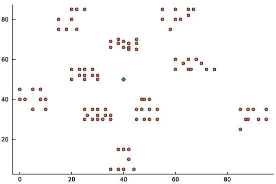
Figure 1.
Distribution of customers (represented by circles) in C-instances with diamond representing the center.
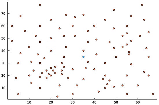
Figure 2.
Distribution of customers (represented by circles) in R-instances with diamond representing the center.
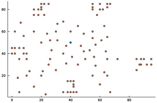
Figure 3.
Distribution of customers (represented by circles) in RC-instances with diamond representing the center.
Table 2.
Literature review for VRPTW with various objective functions and their proposed algorithms.
3. Mathematical Modeling
As mentioned earlier, home visiting in a HHC system can be formulated as a VRPTW problem, which can then be written as a complete graph, having being customers (or patients) where is the starting point of the route. The set , the edges in the graph, represents the travelling connections between nodes. The travel times between points and service time at each point are given. Since the medical needs of patients or customers are unique and may be time-bound, if the service providers (or caretakers) arrive before the specified time window, they will have to wait until the appropriate time. This problem is considered a hard time windows problem. The model constructed here has the objective to minimize total travel costs with the constraints to meet all the traveling/service/matching conditions. The proposed model can be described as follows:
Indices:
- :
- the starting point of the route (called the origin or the health center)
- :
- patients
- :
- the caretaker
Parameters:
- :
- the travel time from patient to patient
- :
- the service time of caretaker at patient
- :
- the earliest starting time (or availability time) of patient
- :
- the latest start time of patient
- :
- the demand of patient
- :
- the capacity of all vehicles
- :
- a compatible matching matrix whose element means patient can be treated by caretaker otherwise
- :
- a large number
Variables:
- :
- equal to 1 if caretaker travels from the origin to patient ; otherwise, 0
- :
- equal to 1 if caretaker travels from node to patient ; otherwise, 0
- :
- equal to 1 if patient is the last patient visited by caretaker ; otherwise, 0
- :
- variables for subtour elimination
- :
- the starting time of patient
- :
- the traveled cost between patient and patient
Mathematical Model
Given a set of patients where represents depot node, a set of caretakers and a set of time windows corresponding to the caretakers, the objective is to find a route for each caretaker to start and return to the origin, with all patients needing to be visited only once with a minimum total cost. Each caretaker must start the job within the time window. This HHC problem can be formulated as a mixed-integer linear programming (MILP):
subject to
With the objective function being to minimize total costs, constraints (1) and (2) are to make sure that each caretaker starts and ends their route at the origin. Constraints (3) and (4) make sure that, for each patient, there is only one caretaker visit and departure. Similarly, constraints (5) ensure that a caretaker leaves a patient for the next one after completing service to the first patient. Constraints (6) are the compatibility constraints to guarantee that only a caretaker compatible with the patient will travel and take care of that patient. Constraints (7) and (8) are the subtour elimination constraint together with capacity constraints. Constraints (9) will activate when caretaker travels from patient to patient (). The completion time of patient (sum of starting time, service duration and travel time) must be less than the starting time of patient . Constraints (10) are time window constraints. Constraints (11) ensure integrality of variables. Finally, is a sufficiently large number.
4. Algorithms
VRPTW is complicated and becomes even more so when some specific constraints, in this case compatibility-matching constraints, are added. We therefore construct a local search to use along with the help of PSO and R&R to solve the problem. Given the discrete nature of our problem, the moving directions in the PSO initially used to solve the continuous optimization problem can be adapted using our developed local search, R&R, and PSO (path relinking procedure). The local search and R&R represent the effect of the individual particle’s cognitive behavior, while the path relinking describes the impact of global social learning behavior which allows a jump out of the local optimum.
Note that the feasibility of solution (particle) can be checked by substituting the particle’s binary representation into the proposed mathematical model. Due to the complexity caused by the presence of time windows, it is difficult to randomly generate a feasible solution (particle). To solve this issue, after the random solution (which is probably infeasible) is obtained, the patients that cause solution infeasibility (arrival time lies outside the time window) are removed. Then the Inserting procedure, described below, is applied to reinsert the patients. The removed patients are added to each caretaker until there is no available place left. If there is still a patient left, a new caretaker is deployed, and the Inserting procedure is applied until there is no patient left to schedule.
Note that the constructed heuristic can be applied, with only slight modifications, to any VRPTW. All steps in the proposed heuristic remain the same, but the feasibility check is based on the characteristics of the new problem. In a similar manner to the feasibility check, the calculation of objective value can be adjusted to satisfy the new problem.
The main algorithm along with all sub-procedures are given in detail below.
4.1. Main Algorithm
PSO is a population-based algorithm for solving an optimization problem which simulates the social behavior of the birth flock. Each individual, called a particle, represents a feasible solution. The particles try to find a direction to the best new solution iteratively around the search space using the information guided by themselves and the best-known best solution.
Let be the population size, be the number of R&R runs, be the maximum number of iterations, be the set of all particles, and be the objective value (i.e., total cost) of particle , for . The pseudocode of the main algorithm based on PSO is given below.
| Main Algorithm | ||||
| 1. | Set parameters: , the number of R&R runs (), and maximum number of iterations | |||
| 2. | Initial step: | |||
| 3. | For do | |||
| 4. | If is infeasible do | |||
| 5. | that make the schedule infeasible | |||
| 6. | Insert the removed patients into the remaining schedule using the Inserting procedure | |||
| 7. | End If | |||
| 8. | End For | |||
| 9. | End Initial step | |||
| 10. | Calculate best-known solution (particle), | |||
| 11. | While and the best particle does not change for 10 iterations | |||
| 12. | Apply Local search procedure to each particle | |||
| 13. | Apply Path relinking procedure to each particle | |||
| 14. | (line 10) | |||
| 15. | If does not change for iterations do | |||
| 16. | Apply the R&R procedure | |||
| 17. | End If | |||
| 18. | End While | |||
| 19. | Return | |||
4.2. Path Relinking Procedure
Path relinking is a search strategy guided by the other solution based on the idea that quality solutions may share similar properties [44]. The guide solution is selected from the current best solution.
Path relinking aims to create a new solution that shares information from the original and the guided solutions. In the context of VRPTW, the good solutions may retain some routes as the current best solution. Route-based path relinking is therefore considered in this study: the new solution will have one of the routes as the guided solution. The path relinking contains two steps. The first step is to select a guided route (any route) from the guided solution and then remove all patients corresponding to the guided route from the current solution. The next step is to insert the removed patients into the current solution using the Inserting procedure. Suppose, for example, that the current solution contains 3 routes arranged as follows: O-A1-A2-A3-A4-O, O-B1-B2-B3-O, O-C1-C2-C3-C4-C5-O, and the guided route is O-A2-B3-A3-C5-O. The result will contain 4 routes: O-A2-B3-A3-C5-O (the guided route), O-A1-A4-O, O-B1-B2-O, and O-C1-C2-C3-C4-O. The procedure can be summarized as follows:
| Path Relinking Procedure | |
| 1. | Input: the current solution, set to and guided solution (current best solution), set to |
| 2. | Randomly choose any route in |
| 3. | Remove all jobs corresponding to route . If the remaining schedule is infeasible, move the infeasible patient to . |
| 4. | Apply the Inserting procedure to insert all jobs in |
4.3. Inserting Procedure
The aim of this procedure is to arrange patients, one by one, between pairs of already assigned patients where none of the assigned patients are served late. In the iteration process, if the inserted patient cannot be treated immediately after the completion time of the directly preceding patient, that caretaker will wait until the lower time window of the patient is reached. A patient that cannot be inserted into any position will be considered a tardy (late) patient.
Let be a set of assigned patients, be a set of tardy patients, be a set of remaining unattended patients and let be a set of all assignments obtained by inserting patient between every pair of patients in the assignment , iteratively. The inserting procedure can be described as follows:
| Inserting Procedure | |||
| 1. | Input: A set of assigned patients, set to , and a set of patients (waiting to be scheduled), set to | ||
| 2. | Set and arrange the patients in according to their upper time windows in ascending order | ||
| 3. | While do | ||
| 4. | Choose the first patient in | ||
| 5. | Consider the set of assignments | ||
| 6. | If there is more than one assignment and all patients are not late do | ||
| 7. | Choose the case that has the minimum completion time, set to | ||
| 8. | Else If there is a tardy patient in every assignment in do | ||
| 9. | Choose the assignment with only one late patient, set as | ||
| 10. | Else If has more than two tardy patients do | ||
| 11. | |||
| 12. | End If | ||
| 13. | End While | ||
| 14. | While do | ||
| 15. | Add a new caretaker. Repeat all steps in the While loop with , until there is no change in . | ||
| 16. | End While | ||
4.4. Local Search Procedure
The aim of the proposed Local Search is to improve the solution. Some patients, if served by a different caretaker, could result in reduced objective value. Since there are many candidates to consider, it is more convenient to generate a priority list of every pair of jobs. The List is sorted using the traveling times between pairs of patients in ascending order.
We developed three improving procedures: Swapping procedure (Section 4.4.1), Moving procedure (Section 4.4.2), and 2-opt procedure (Section 4.4.3). In the first step of Local Search, the procedure will generate a priority list containing all candidates for swapping, moving, and 2-opt. It will then apply Swapping, Moving and 2-opt procedures accordingly. The procedures are explained in detail below.
4.4.1. Swapping Procedure
The swapping procedure aims to switch the order of a pair of jobs on the List in order to make the solution better, or to reduce the objective value. For our purpose, the List is generated by sorting travel times between pairs of patients. This procedure will be applied multiple times until the solution can no longer be improved.
| Swapping Procedure | ||
| 1. | For (job1, job2) in List do | |
| 2. | swap the routing position between job1 and job2 if it reduces the total routing cost and the routing is still feasible. | |
| 3. | End For | |
4.4.2. Moving Procedure
This procedure uses the same idea as the swapping procedure: the chosen patient is moved to another position. The patient moves when the objective value is reduced; otherwise, the patient will maintain his/her position. This procedure also uses the same List as the swapping procedure.
| Moving Procedure | ||
| 1. | For (job1, job2) in List do | |
| 2. | Move job2 to process before or after job1 if it reduces the total routing cost and the routing is feasible. If both positions reduce cost, choose the one with more cost reduction. | |
| 3. | End For | |
4.4.3. 2-Opt Procedure
This is a local search procedure for solving the traveling salesman problem. It uses the same idea as the swapping procedure by swapping a pair of edges, instead of patients, from any route and reconnecting them with each other. In other words, the main idea is the crossover between two routes. The edge moves when the objective value is reduced; otherwise, all patients will maintain their positions. The List for this procedure contains all pairs of edges in random order. Suppose, for example, that we have two routes that start and end at the origin, denoted by “O”, and are arranged as follows: O-A1-A2-A3-A4-A5-O and O-B1-B2-B3-B4-B5-B6-O. Suppose the selected edges are (A1-A2) and (B4-B5). The result routes will be O-A1-B5-B6-O and O-B1-B2-B3-B4-A2-A3-A4-A5-O.
| 2-Opt Procedure | ||
| 1. | For (A-B, C-D) in List do | |
| 2. | Define a path starting from depot to node A by OA, a path starting from B to depot by BO, a path starting from depot to node C by OC, and a path starting from D to depot by DO. | |
| 3. | Reconstruct a path as OA connected to DO and OC connected to BO only if the result is feasible and the total cost is reduced. | |
| 4. | End For | |
4.5. R&R Procedure
The main idea behind this procedure is to jump out to a new solution to avoid the local optimum [30]. In this procedure, one of the caretakers is randomly removed. The removed patients are then added to the remaining caretakers using the Inserting procedure. If some of the remaining patients cannot be inserted into any place, a new caretaker will be deployed by applying the Inserting procedure to the remaining patients.
| R&R Procedure | ||
| 1. | Input: Routing solution | |
| 2. | Randomly select a caretaker, set to , and remove all patients belonging to that caretaker from the routing solution. | |
| 3. | For do | |
| 4. | by applying the Inserting procedure to each caretaker; if there is no place to insert, deploy a new caretaker and apply the procedure again | |
| 5. | End For | |
5. Computational Results on Solomon’s Instances
To test our constructed heuristic, we apply it to solve the well-known benchmark instances called Solomon’s instances with 25, 50, and 100 customers. As mentioned earlier, there are 3 groups of instances, C (clustered), R (random) and RC (randomly clustered). The parameters used in all simulation results are: number of particles, set at 15 (); number of R&R runs, which is 5 (); and maximum iterations, set at 500 (). These parameters greatly affect the performance of the heuristic. For example, if the number of particles is high, the objective function value tends to be better. However, we will have to sacrifice the time needed to execute each iteration. Since a higher number of particles does not guarantee a better solution, we limit the number of particles to 15 where the running time is comparatively low. The number of R&R is set to 5 in an attempt to diversify particles when they have similar solutions or similar route. This normally occurs when the heuristic reaches a local optimum, since the path relinking process tends to move all particles that are similar to each other. As for the maximum number of iterations, in all problems tested this has never reached 500, hence the number is set to 500.
To illustrate the proposed heuristic’s performance, the heuristic is written in Julia’s language [45,46] and run on AMD Ryzen 9 12-Core processors with 3.8 GHz CPU and 64 GB of RAM. The results shown in Table 3, Table 4 and Table 5 compare the optimum objective function values and that obtained with our heuristic for the Solomon’s instances with 25, 50, and 100 customers, respectively. For those instances where the optimal solutions have not been found in the existing literature, we compare our results with the best solutions from the literature. The number of vehicles presented is equivalent to the number of caretakers. The customers presented can be seen as the patients. The “%Gap” is the percentage difference between the values obtained with our heuristic and the optimal values. With 52, 21, and 18 out of 56 cases that our heuristic can find the optimal solutions in 25, 50, and 100 customer instances, we can say that our heuristic performs better in smaller-size instances. In general, our heuristic performs better in C1 and C2 instances since the %Gap is smaller compared to the R1, R2, RC1, and RC2 instances. Moreover, in most cases the optimal solutions have yet to be found, and the %Gap is less than 5%.
Table 3.
Comparisons between the exact solutions and the results obtained by our heuristic on 25-customer Solomon instances.
Table 4.
Comparisons between the exact solution or best solutions (with “*”) and the results obtained by our heuristic on 50-customer Solomon instances.
Table 5.
Comparisons between the exact solution or best solutions (with “*”) and the results obtained by our heuristic on 100-customer Solomon instances.
Note that for all computations, the distance between each pair of nodes is truncated to 1 digit. It is also worth mentioning that the running time for each iteration on 25-customer instances is recorded at approximately 1 s for RC2 instances (at 20 total number of iterations), 2 s for all C1, R1, R2, and RC1 instances (at 10, 10, 12, and 20 iterations), and 3 s for C2 instances (at 15 iterations). The running times for each iteration on 50 customer instances are 4 s for C1 (at 25 iterations), 5 s for R2 and RC2 (at 25 and 30 iterations), and 6, 7, and 10 s for R1, RC1, and C2 instances (at 20, 25, and 30 iterations), respectively. For those instances with 100 customers, the running time for each iteration is recorded at approximately 30 s for all C1 instances, and 1 min for C2, R1, R2, RC1, and RC2 instances. Note that the running time depends on the number of particles and maximum iterations set. However, for each instance, the heuristic executes with the indicated solution after only a few iterations (for the worst case, up to 30 iterations or up to 30 min for each instance).
To further analyze the performance of our heuristic, we modify Solomon’s instances to contain compatibility between patients and caretakers. The solutions obtained with our heuristic are shown in Table 6 along with the optimal solutions. Note the negative %Gap in the first instance: this is because our heuristic cannot find a feasible solution with 3 vehicles. The optimal solutions can be found for only 5 out of 56 cases. This indicates that the difficulty level of the problem has increased dramatically. Note that the computation time of the instances with compatibility is the same as without compatibility constraints.
Table 6.
Comparison between the exact solution of Solomon’s instances with and without compatibility, and the solution with compatibility obtained with our algorithm.
6. Conclusions
In this paper, we formulated mathematical modeling and a heuristic for solving a home healthcare routing and scheduling problem in which caretakers must visit specific patients within a specific time frame. This problem can be formulated into a vehicle routing problem with time windows (VRPTW) and compatibility constraints.
Due to the NP-hard nature of the problem, we presented a new heuristic combining particle swarm optimization, inserting procedure, local search, path relinking, and ruin-and-recreate (R&R) procedures. In particular, the inserting procedure is used to generate initial solutions and restore the feasibility of the solution. The constructed local search procedure representing the particle’s movement to the local space is used to improve the solutions. Path relinking represents the global search movement of particles; at each iteration, the procedure is used to improve the current solution by integrating the current solution with the current best solution. R&R is deployed in cases where leaping out of the local optimum is necessary.
To test the performance of the heuristic, we applied it to Solomon’s instances with 25, 50 and 100 customers and compared objective values obtained with our heuristic and the optimum values collected from published literature. Computational results show that our proposed heuristic performs better on smaller instances and in all clustered problems (C1 and C2 instances). Further investigation with compatibility constraints included in the model shows that our proposed heuristic also performed very well on 25 customer instances yielding solutions with less than 10% optimality gap. However, only 5 optimal solutions are found in the model with compatibility constraints compared with 52 optimal solutions found in the model without the constraints. This also suggests that the problem is much more difficult compared with regular VRPTW.
The parameters in this study are experimentally selected to balance the computation time and solution quality. This does not guarantee the best performance of the algorithm. Moreover, as searching for the parameters is very time-consuming, one could consider the parameterized metaheuristic as presented in [52].
Author Contributions
Conceptualization, P.S. and C.L.; Data curation, P.S.; Formal analysis, C.L.; Investigation, P.S.; Methodology, P.S. and C.L.; Software, P.S.; Supervision, C.L.; Validation, P.S. and C.L.; Visualization, C.L.; Writing—original draft, P.S.; Writing—review and editing, C.L. All authors have read and agreed to the published version of the manuscript.
Funding
This research is supported by the Royal Golden Jubilee Ph.D. Program [Grant No. PHD/0041/2560]; and the Research Group in Mathematics and Applied Mathematics, Department of Mathematics, Faculty of Science, Chiang Mai University.
Institutional Review Board Statement
Not applicable.
Informed Consent Statement
Not applicable.
Data Availability Statement
Not applicable.
Acknowledgments
The authors thanks the Royal Golden Jubilee Ph.D. Program, and the Research Group in Mathe-matics and Applied Mathematics, Department of Mathematics, Faculty of Science, Chiang Mai University for the support. The authors appreciate Wiriya Sungkhaniyom for her proofreading help.
Conflicts of Interest
The authors declare no conflict of interest.
References
- United Nations. World Population Prospects 2019, Volume II: Demographic Profiles; Department of Economic and Social Affairs: New York, NY, USA, 2019. [Google Scholar]
- Office of the National Economic and Social Development Board Office of the Prime Minister Bangkok Thailand. Summary the Twelfth National Economic and Social Development Plan (2017–2021); Office of the National Economic and Social Development Board Office of the Prime Minister: Bangkok, Thailand, 2017.
- Suriyanrattakorn, S.; Chang, C.-L. Long-Term Care (LTC) Policy in Thailand on the Homebound and Bedridden Elderly Happiness. Health Policy Open 2021, 2, 100026. [Google Scholar] [CrossRef]
- Wirnitzer, J.; Heckmann, I.; Meyer, A.; Nickel, S. Patient-Based Nurse Rostering in Home Care. Oper. Res. Health Care 2016, 8, 91–102. [Google Scholar] [CrossRef]
- Braekers, K.; Hartl, R.F.; Parragh, S.N.; Tricoire, F. A Bi-Objective Home Care Scheduling Problem: Analyzing the Trade-off between Costs and Client Inconvenience. Eur. J. Oper. Res. 2016, 248, 428–443. [Google Scholar] [CrossRef] [Green Version]
- Ait Haddadene, S.R.; Labadie, N.; Prodhon, C. A GRASP × ILS for the Vehicle Routing Problem with Time Windows, Synchronization and Precedence Constraints. Expert Syst. Appl. 2016, 66, 274–294. [Google Scholar] [CrossRef]
- Polnik, M.; Riccardi, A.; Akartunalı, K. A Multistage Optimisation Algorithm for the Large Vehicle Routing Problem with Time Windows and Synchronised Visits. J. Oper. Res. Soc. 2021, 72, 2396–2411. [Google Scholar] [CrossRef]
- Yu, M.; Nagarajan, V.; Shen, S. An Approximation Algorithm for Vehicle Routing with Compatibility Constraints. Oper. Res. Lett. 2018, 46, 579–584. [Google Scholar] [CrossRef]
- Riazi, S.; Wigstrom, O.; Bengtsson, K.; Lennartson, B. A Column Generation-Based Gossip Algorithm for Home Healthcare Routing and Scheduling Problems. IEEE Trans. Autom. Sci. Eng. 2019, 16, 127–137. [Google Scholar] [CrossRef]
- Kandakoglu, A.; Sauré, A.; Michalowski, W.; Aquino, M.; Graham, J.; McCormick, B. A Decision Support System for Home Dialysis Visit Scheduling and Nurse Routing. Decis. Support Syst. 2020, 130, 113224. [Google Scholar] [CrossRef]
- Nasir, J.A.; Kuo, Y.-H. A Decision Support Framework for Home Health Care Transportation with Simultaneous Multi-Vehicle Routing and Staff Scheduling Synchronization. Decis. Support Syst. 2020, 138, 113361. [Google Scholar] [CrossRef]
- Cissé, M.; Yalçındağ, S.; Kergosien, Y.; Şahin, E.; Lenté, C.; Matta, A. OR Problems Related to Home Health Care: A Review of Relevant Routing and Scheduling Problems. Oper. Res. Health Care 2017, 13–14, 1–22. [Google Scholar] [CrossRef]
- di Mascolo, M.; Martinez, C.; Espinouse, M.-L. Routing and Scheduling in Home Health Care: A Literature Survey and Bibliometric Analysis. Comput. Ind. Eng. 2021, 158, 107255. [Google Scholar] [CrossRef]
- Solomon, M.M. Algorithms for the Vehicle Routing and Scheduling Problems with Time Window Constraints. Oper. Res. 1987, 35, 254–265. [Google Scholar] [CrossRef] [Green Version]
- Larsen, J. Parallelization of the Vehicle Routing Problem with Time Windows; Technical University of Denmark: Kongens Lyngby, Danmark, 1999. [Google Scholar]
- Kallehauge, B.; Larsen, J.; Madsen, O.B.G. Lagrangean Duality Applied on Vehicle Routing with Time Windows Experimental Results. In IMM-Technical Report-2001-9; Informatics and Mathematical Modelling, Technical University of Denmark: Lyngby, Denmark, 2001. [Google Scholar]
- Cook, W.; Rich, J.L. A Parallel Cutting-Plane Algorithm for the Vehicle Routing Problem with Time Windows. In CAAM Technical Reports; Digital Scholarship Services: Houston, TX, USA, 1999. [Google Scholar]
- Rochat, Y.; Taillard, É.D. Probabilistic Diversification and Intensification in Local Search for Vehicle Routing. J. Heuristics 1995, 1, 147–167. [Google Scholar] [CrossRef]
- Ombuki, B.; Ross, B.J.; Hanshar, F. Multi-Objective Genetic Algorithms for Vehicle Routing Problem with Time Windows. Appl. Intell. 2006, 24, 17–30. [Google Scholar] [CrossRef]
- Alvarenga, G.B.; Mateus, G.R.; de Tomi, G. A Genetic and Set Partitioning Two-Phase Approach for the Vehicle Routing Problem with Time Windows. Comput. Oper. Res. 2007, 34, 1561–1584. [Google Scholar] [CrossRef]
- Zbigniew, J.C. Best Solutions Found by the Parallel Simulated Annealing Algorithm for Solomon’s Vehicle Routing Problem with Time Windows (VRPTW) Benchmark Instances. Available online: http://sun.aei.polsl.pl/~zjc/best-solutions-solomon.html (accessed on 6 June 2021).
- Khoo, T.S.; Mohammad, B.B. The Parallelization of a Two-Phase Distributed Hybrid Ruin-and-Recreate Genetic Algorithm for Solving Multi-Objective Vehicle Routing Problem with Time Windows. Expert Syst. Appl. 2021, 168, 114408. [Google Scholar] [CrossRef]
- Jung, S.; Moon, B.-R. A Hybrid Genetic Algorithm for the Vehicle Routing Problem with Time Windows. In Proceedings of the Proceedings of the 4th Annual Conference on Genetic and Evolutionary Computation, New York, NY, USA, 9–13 July 2002; pp. 1309–1316. [Google Scholar]
- Ahn, B.-H.; Shin, J.-Y. Vehicle-Routeing with Time Windows and Time-Varying Congestion. J. Oper. Res. Soc. 1991, 42, 393. [Google Scholar] [CrossRef]
- Eshtehadi, R.; Demir, E.; Huang, Y. Solving the Vehicle Routing Problem with Multi-Compartment Vehicles for City Logistics. Comput. Oper. Res. 2020, 115, 104859. [Google Scholar] [CrossRef]
- Low, C.; Chang, C.-M.; Li, R.-K.; Huang, C.-L. Coordination of Production Scheduling and Delivery Problems with Heterogeneous Fleet. Int. J. Prod. Econ. 2014, 153, 139–148. [Google Scholar] [CrossRef]
- Chen, J.; Shi, J. A Multi-Compartment Vehicle Routing Problem with Time Windows for Urban Distribution—A Comparison Study on Particle Swarm Optimization Algorithms. Comput. Ind. Eng. 2019, 133, 95–106. [Google Scholar] [CrossRef]
- Shaw, P. A New Local Search Algorithm Providing High Quality Solutions to Vehicle Routing Problems; APES Group, Dept of Computer Science, University of Strathclyde: Glasgow, UK, 1997. [Google Scholar]
- Shaw, P. Using Constraint Programming and Local Search Methods to Solve Vehicle Routing Problems. In International Conference on Principles and Practice of Constraint Programming; Springer: Berlin/Heidelberg, Germany, 1998; pp. 417–431. [Google Scholar]
- Schrimpf, G.; Schneider, J.; Stamm-Wilbrandt, H.; Dueck, G. Record Breaking Optimization Results Using the Ruin and Recreate Principle. J. Comput. Phys. 2000, 159, 139–171. [Google Scholar] [CrossRef] [Green Version]
- Rousseau, L.-M.; Gendreau, M.; Pesant, G. Using Constraint-Based Operators to Solve the Vehicle Routing Problem with Time Windows. J. Heuristics 2002, 8, 43–58. [Google Scholar] [CrossRef]
- Li, H.; Lim, A. Local Search with Annealing-like Restarts to Solve the VRPTW. Eur. J. Oper. Res. 2003, 150, 115–127. [Google Scholar] [CrossRef]
- Berger, J.; Barkaoui, M. A Parallel Hybrid Genetic Algorithm for the Vehicle Routing Problem with Time Windows. Comput. Oper. Res. 2004, 31, 2037–2053. [Google Scholar] [CrossRef]
- Mester, D.; Bräysy, O.; Dullaert, W. A Multi-Parametric Evolution Strategies Algorithm for Vehicle Routing Problems. Expert Syst. Appl. 2007, 32, 508–517. [Google Scholar] [CrossRef]
- Pisinger, D.; Ropke, S. A General Heuristic for Vehicle Routing Problems. Comput. Oper. Res. 2007, 34, 2403–2435. [Google Scholar] [CrossRef]
- Marinakis, Y.; Marinaki, M.; Migdalas, A. A Multi-Adaptive Particle Swarm Optimization for the Vehicle Routing Problem with Time Windows. Inf. Sci. 2019, 481, 311–329. [Google Scholar] [CrossRef]
- Gehring, H.; Homberger, J. A Parallel Hybrid Evolutionary Metaheuristic for the Vehicle Routing Problem with Time Windows. In Proceedings of the EUROGEN99; Springer: Berlin/Heidelberg, Germany, 1999; pp. 57–64. [Google Scholar]
- Bent, R.; van Hentenryck, P. A Two-Stage Hybrid Local Search for the Vehicle Routing Problem with Time Windows. Transp. Sci. 2004, 38, 515–530. [Google Scholar] [CrossRef] [Green Version]
- Repoussis, P.P.; Tarantilis, C.D.; Ioannou, G. Arc-Guided Evolutionary Algorithm for the Vehicle Routing Problem With Time Windows. IEEE Tran. Evol. Comput. 2009, 13, 624–647. [Google Scholar] [CrossRef]
- Galindres-Guancha, L.F.; Toro-Ocampo, E.; Gallego-Rendón, R. A Biobjective Capacitated Vehicle Routing Problem Using Metaheuristic Ils and Decomposition. Int. J. Ind. Eng. Comput. 2021, 12, 293–304. [Google Scholar] [CrossRef]
- Gambardella, L.M.; Taillard, É.; Agazzi, G. MACS-VRPTW: A Multiple Ant Colony System for Vehicle Routing Problems with Time Windows. In New Ideas in Optimization; McGraw-Hill: London, UK, 1999; pp. 63–76. [Google Scholar]
- Expósito, A.; Brito, J.; Moreno, J.A.; Expósito-Izquierdo, C. Quality of Service Objectives for Vehicle Routing Problem with Time Windows. Appl. Soft Comput. 2019, 84, 105707. [Google Scholar] [CrossRef]
- Taillard, É.; Badeau, P.; Gendreau, M.; Guertin, F.; Potvin, J.-Y. A Tabu Search Heuristic for the Vehicle Routing Problem with Soft Time Windows. Transp. Sci. 1997, 31, 170–186. [Google Scholar] [CrossRef] [Green Version]
- Glover, F.; Manuel, L. Rafael Martí Fundamentals of Scatter Search and Path Relinking. Control Cybern. 2000, 29, 653–684. [Google Scholar]
- Bezanson, J.; Karpinski, S.; Shah, V.B.; Edelman, A. Julia: A Fast Dynamic Language for Technical Computing. arXiv 2012, arXiv:1209.5145. [Google Scholar] [CrossRef]
- Bezanson, J.; Edelman, A.; Karpinski, S.; Shah, V.B. Julia: A Fresh Approach to Numerical Computing. SIAM Rev. 2017, 59, 65–98. [Google Scholar] [CrossRef] [Green Version]
- Kohl, N. 2-Path Cuts for the Vehicle Routing Problem with Time Windows. Transp. Sci. 1999, 33, 101–116. [Google Scholar] [CrossRef]
- Irnich, S.; Villeneuve, D. The Shortest-Path Problem with Resource Constraints and k-Cycle Elimination for k ≥ 3. Inf. J. Comput. 2006, 18, 391–406. [Google Scholar] [CrossRef] [Green Version]
- Chabrier, A. Vehicle Routing Problem with Elementary Shortest Path Based Column Generation. Comput. Oper. Res. 2006, 33, 2972–2990. [Google Scholar] [CrossRef]
- Hedar, A.-R.; Bakr, M.A. Three Strategies Tabu Search for Vehicle Routing Problem with Time Windows. Comput. Sci. Inf. Technol. 2014, 2, 108–119. [Google Scholar] [CrossRef]
- Danna, E.; le Pape, C. Branch-and-Price Heuristics: A Case Study on the Vehicle Routing Problem with Time Windows. In Column Generation; Springer: Boston, MA, USA, 2005; pp. 99–129. [Google Scholar] [CrossRef]
- Cutillas-Lozano, J.M.; Giménez, D.; Almeida, F. Hyperheuristics based on parametrized metaheuristic schemes. In Proceedings of the 2015 Annual Conference on Genetic and Evolutionary Computation, Madrid, Spain, 11–15 July 2015; pp. 361–368. [Google Scholar]
Publisher’s Note: MDPI stays neutral with regard to jurisdictional claims in published maps and institutional affiliations. |
© 2022 by the authors. Licensee MDPI, Basel, Switzerland. This article is an open access article distributed under the terms and conditions of the Creative Commons Attribution (CC BY) license (https://creativecommons.org/licenses/by/4.0/).