Wavelet Time-Scale Modeling of Brand Sales and Prices

Abstract

Marketing is the way we ensure our sales are the best in the market, our prices the most accessible, and our clients satisfied, thus ensuring our brand has the widest distribution. This requires sophisticated and advanced understanding of the whole related network. Indeed, marketing data may exist in different forms such as qualitative and quantitative data. However, in the literature, it is easily noted that large bibliographies may be collected about qualitative studies, while only a few studies adopt a quantitative point of view. This is a major drawback that results in marketing science still focusing on design, although the market is strongly dependent on quantities such as money and time. Indeed, marketing data may form time series such as brand sales in specified periods, brand-related prices over specified periods, market shares, etc. The purpose of the present work is to investigate some marketing models based on time series for various brands. We will precisely study the effect of the time scale on the persistence of brand sales in the market and on the forecasting of such persistence, according to the characteristics of the brand and the related market competition or competitors. Our study is based on a sample of Saudi brands during the period 22 November 2017 to 30 December 2021.

1. Introduction

The aim of this work is to investigate a wavelet-based mathematical model for brand sales and prices. Wavelet theory has gained great interest in the fields of economics and finance since the last decades of the last century. Recall that almost all financial indices usually show volatile behavior as well as high fluctuations. As a result, their investigation using classical methods remains insufficient. Wavelets have indeed been shown to be useful in such investigations.

Marketing, in its simplest sense, includes the institutions, the activities, and also the processes applied to deliver, create, and exchange goods, and to communicate offerings and needs to customers, partners, and clients, or more broadly to society [1]. While marketing consists of various activities, the principles of marketing rely on four elements, i.e., product, price, promotion, and place (distribution). Each one of these elements depends on qualitative and quantitative data. Quantitative data show the power of marketing in collecting, analyzing, optimizing, and executing, based on relevant numerical data. Product choices and portfolios, price hierarchies, numbers of outlets and stores, and, importantly, promotion budgets, especially for branding, brand management, and brand equity are also considered. Brands and the activity of branding are well represented in the literature, and brand equity refers to the value added to products [2]. Firms can benefit from a strong brand in various ways: it improves the product value and provides a chance to extend the brand to new products, expand into new markets, and obtain a high level of customer loyalty and tolerance. A well-known brand acquires a price value [3]. Thus, brand sales- and equity-related data include things such as choice data, the brand design, the brand idea, time of purchases, the number of stores, the choice of price, and the competitors in the market. The state of the market itself affects the persistence and the success of the brand investment, strongly and simultaneously. Without sophisticated mathematical models that take into account all the factors and that permit a good understanding of the time and space evolution of the brand distribution and its evolution in the market, the investment in the brand may fail.

In marketing, a mathematical model may include many factors such as the number of sales in specified periods such as weeks, months, or years, market shares per specified period, price evolution, the history of the market and its situation, competing brands, etc. The main characteristic of a mathematical model is its ability to deal with many factors simultaneously, according to time and space. It gathers the data into a time series form, permitting ordering over time. This has a very important consequence, as it yields information about the future state of the brand. The model uses a time series, as the best descriptor to extract, deduce, and/or accurately describe the properties of the empirical data.

In the present paper, we aim to investigate the multidimensional modeling of time series obtained from brand sales and the evolution of prices. The model is of a general form, including many variables such as sales, prices, and advertising simultaneously. Our principal idea is based on the effect of the time factor on the brand evolution. In [4,5], the authors mention that one of the limitations of conventional approaches in economic or financial studies and models is the lack of dependence of the models on the time scale, taking into account both the frequency and time domains. These facts are of great importance for the economic/econometric rationale.

In many scientific fields, wavelets have provided efficient reformulations of many difficult problems such as the analysis and the modeling of time series, by transforming data from time domains to levels or horizons, according to the frequency. Their main advantage is their ability to be localized in the time/frequency domain. These characteristics of wavelet tools result in efficient algorithms in practice, outperforming classical techniques. Readers may refer, for instance, to [6,7,8,9,10,11,12,13,14].

In the present paper, we aim to use wavelets to improve and understand mathematical models for brand marketing. The validity of the models will enable effective decisions by financial managers, as well as analysts and decision makers. One of the major factors, indeed, is the security valuation accuracy.

The next section concerns the literature review of existing studies on marketing models. Section 3 reviews the wavelet toolkit. Section 4 is devoted to the development of our main mathematical modeling system. Section 5 concerns the empirical results, together with a discussion and interpretations. Section 6 concludes the paper.

2. Literature Review

Generally, marketing researchers and/or modelers search for models taking into account one or more variables solely as functions of time. Next, the model is analyzed regarding its efficiency for interpolating (approximating) and extrapolating (predicting) these variables in time.

Compared to other fields such as financial and economic applications, the use of mathematical models, especially wavelet-based models, is still not well developed in marketing. In [15], for example, the authors mention the difficulty of time series training for traditional research models, the lack of software adapted to marketing modeling, the lack of, and sometimes the poor quality of, time-series data, and the lack of a substantive area for marketing, allowing time-series-based models to be readily adopted.

The problem of time scales in marketing has been raised in several studies. In [16], it is mentioned that marketing phenomena depend on frequencies in time relative to decisions and interactions in the market. In classical investigations, the most commonly used time intervals are weekly, monthly, quarterly, and annual cycles. Each period has its special and/or specific characteristics. Weekly cycles, for example, are for reductions in prices, and quarterly periods are generally related to regular price adjustments and competition.

Moreover, many phenomena such as pandemics (COVID-19), wars, climate change, financial crises, and socio-political movements may induce severe perturbations in the usual considerations, especially time periods, leading to diversification in the use of time scales.

This diversification in how to choose the time scale, according to what factors, what characteristics, and what aim, has led researchers in the marketing field to think about including the time scale strongly in the models. In [17], the authors applied certain types of short-, medium-, and long-term horizons to investigate the effect of the time scale. However, their choice was not adapted to the wavelet method.

In marketing, according to [16,18], the time scale is mostly applied at discrete, equally spaced intervals, with weekly periods dominating, although this hypothesis has been criticized. In [18], the author applied a wavelet-based method for forecasting brand sales. The problem of multicollinearity has been investigated, resulting in correlated vectors of coefficients which have been applied to provide the most accurate forecasting and the best dimension reduction. In [19], for example, it is mentioned that marketing models still present aggregations, even using weekly intervals. This allows us to conclude that more adequate tools for time/frequency scales should be applied.

Many methods have been used in this context, such as Fourier analysis and spectral analysis [20,21]. However, these tools have raised many problems such as the non-stationary behavior of the marketing data, the sizes of samples, etc. (see also [22,23,24,25,26,27]).

Wavelet analysis was introduced into marketing models to overcome limitations such as the non-localization aspect of spectral analysis and its concentration in the frequency domain. This is achieved by frequency decomposition of the statistical time series into components that are well localized in time/frequency.

Michis mentioned a very important characteristic of wavelet theory in [16,18,28]. It permits investigation of the causal links between time-series cycles in marketing according to time scale. The modelers differentiate the marketing-driver influences in long-duration cycles of sales. Wavelets are also good tools regarding estimation and prediction accuracy and the handling of non-stationary time series. The application of wavelets in marketing resides in covering/uncovering the frequency activity characteristics of marketing models. Wavelet crystals generated from the inverse of the wavelet transform are applied to localize the variation in economic variables over different horizons. Recall that brand sales forecasting is important for investors and consumers but also for modelers, due to its strong relationships with financial resources allocation and budget planning. Therefore, a successful sales forecast will yield a good guide to planning sufficient production and good product distribution, according to both time and demand. Furthermore, appropriate marketing activities will be well organized, resulting in good performance and placement in the market [16,18,28].

3. Wavelets Toolkit

As the literature on wavelets has grown dramatically since their discovery in the last century, we will review wavelet tools briefly in this part of the paper by focusing essentially on time series analysis and/or modeling.

Wavelet analysis allows the representation of time series into forms relative to the time and frequency information, known as time–frequency decomposition. It involves decomposing a series into different frequency components at a scale-adapted resolution and thus allows the data to be observed and analyzed at different scales. The starting point of wavelet analysis is a mother wavelet $\psi$ ($\in L^2\left(\mathbb{R}\right)$, satisfying some appropriate assumptions). Such a mother wavelet yields the so-called wavelet basis $({\psi }_{j,k}=2^{-j/2}\psi (2^j.-k),j,k\in \mathbb{Z})$, where j is known as the scale, frequency, level, or horizon, and k is the position or translation parameter. The mother wavelet $\psi$ gives rise to a second analyzing function called the father wavelet (or also the scaling function) $\phi$. For a fixed $j\in \mathbb{Z}$, we introduce two types of functional spaces:

• The j-level detail space $W_j=span({\psi }_{j,k},k)$;
• The j-level approximation space $V_j=span({\phi }_{j,k},k)$.

These spaces satisfy several useful properties such as

$${\displaystyle L^2\left(\mathbb{R}\right)=\underset{j}{\overset{\perp }{⨁}}{W}_j=\overline{{\displaystyle \bigcup _j{V}_j}}\mathrm{and}{V}_{j+1}=W_j{\oplus }^{\perp }{V}_j,}$$

where ${\phi }_{j,k}$ are defined in the same way as ${\psi }_{j,k}$. The sequence ${\left(V_j\right)}_j$ constitutes the multi-resolution analysis (multi-scale analysis) on $\mathbb{R}$. Details on these concepts may be found in [7,29,30].

Using the above properties of wavelets and wavelet functional spaces, we deduce that any time series $X\left(t\right)$ may be represented as

$${\displaystyle X\left(t\right)=\sum _j{D}_j\left(t\right)=\sum _{j\le J}{D}_j\left(t\right)+\sum _{j\ge J+1}{D}_j\left(t\right)=A_J\left(t\right)+\sum _{j\ge J+1}{D}_j\left(t\right),}$$

(1)

for all $J\in \mathbb{Z}$, where the $D_j\left(t\right)$ is the projection on $W_j$, known as the detail component at level j,

$${\displaystyle D_j\left(t\right)=\sum _k{d}_{j,k}{\psi }_{j,k}\left(t\right),}$$

(2)

and where

$${\displaystyle A_J\left(t\right)=\sum _k{a}_{J,k}{\phi }_{J,k}\left(t\right)=\sum _{j\le J}{D}_j\left(t\right)}$$

(3)

is the projection on $V_j$, known also as the approximation of $X\left(t\right)$ at level J. This describes the global shape or the trend of $X\left(t\right)$. The coefficients

$${\displaystyle d_{j,k}=<X\left(t\right),{\psi }_{j,k}>={\int }_{\mathbb{R}}X\left(t\right){\psi }_{j,k}\left(t\right)dt,}$$

(4)

are known as the detail or wavelet coefficients of the series $X\left(t\right)$ at level j and position k, and the coefficients

$${\displaystyle a_{j,k}=<X\left(t\right),{\phi }_{j,k}>={\int }_{\mathbb{R}}X\left(t\right){\phi }_{j,k}\left(t\right)dt}$$

(5)

are known as the approximation coefficients at level j and position k.

In the case of time series such as brand sales and prices, we use a discrete convolution to evaluate these coefficients:

$$d_{j,k}=\sum _{n}X\left(n\right){\psi }_{j,k}\left(n\right)\mathrm{and}{a}_{j,k}=\sum _{n}X\left(n\right){\phi }_{j,k}\left(n\right).$$

(6)

In the context of marketing, the series $X\left(t\right)$ may represent the prices, volumes, competitive prices, or promotion prices, as will be explained later for the marketing model (8) in Section 4.

As a result, the wavelet series or the decomposition of $X\left(t\right)$ is composed of a first part due to the global shape (the trend) $A_J$, together with the details or the higher-frequency components $D_j$.

For empirical use, we obviously focus on a fixed maximal level J at which we truncate the decomposition:

$${\displaystyle X_J\left(t\right)=A_{J_0}\left(t\right)+\sum _{J_0<j\le J}{D}_j\left(t\right),}$$

(7)

where $J_0<J$. In fact, there is no rule for fixing the levels $J_0$ and J. However, for $J_0$, we always have some flexibility, as it does not affect the total decomposition (we usually take $J_0-0$). The maximal level J is selected relative to the desired error estimates. We know, in fact, that $\parallel X_J{-X\parallel }_2\to 0$ as $J\to \infty$.

In marketing, the wavelet theory and mathematically advanced models in general have still not been widely developed. However, in actuarial sciences such as management, economics, finance, and econometrics, wavelet modeling and analysis are growing rapidly as sophisticated tools recently discovered in these fields, and it may be a useful task to extend wavelet and multi-scale models generally to marketing and business, due to the natural link between these areas and actuarial sciences (see [7,8,9,10,11,12,14,31,32,33,34,35,36,37,38,39,40,41,42,43]).

4. Development of the Mathematical Modeling System

In the literature there are few models relating to marketing. We firstly recall that our aim in the present work is not purely the development of new models but instead the proof of the influence of the time-scale factor on marketing models, as shown in many other contexts in financial and economic studies, thus involving wavelets in the improvement of these models. Our contribution may be seen as the wavelet time-scale generalization and/or extension of existing models by considering scale-by-scale versions. A recent models proposed by Hansenes et al. [44] was adopted to describe the link between brand sales, prices, competitors, and promotions. It states that

$$S_t={\beta }_0+{\beta }_1{P}_t+{\beta }_{2}C{P}_t+{\beta }_{3}P{R}_t+{\beta }_4{D}_t+{ϵ}_t,$$

(8)

where:

• $S_t$ stands for the sales value at time t;
• $P_t$ stands for the price at time t;
• $C{P}_t$ stands for the competitor’s price at time t;
• $P{R}_t$ is the PROMO variable at time t;
• $D_t$ refers to percentage distribution of the main brand;
• ${ϵ}_t$ is an error term.

Using wavelets, we consider a multi-resolution or multi-horizons or levels model, where the variables must be replaced by their projections on the multi-resolution and/or detail spaces, as in (7). Therefore, for any level j, we obtain a j-level model

$$S_{t,j}={\beta }_{0,j}+{\beta }_{1,j}{P}_{t,j}+{\beta }_{2,j}C{P}_{t,j}+{\beta }_{3,j}P{R}_{t,j}+{\beta }_{4,j}{D}_{t,j}+{ϵ}_{t,j},$$

(9)

where:

• $S_{t,j}$ reflects the sales value at time t and the level or horizon j;
• $P_{t,j}$ stands for the price at level j and time t;
• $C{P}_{t,j}$ stands for the competitor’s price at level j and time t;
• $P{R}_{t,j}$ is the PROMO variable at horizon j and time t;
• $D_{t,j}$ stands for the percentage distribution at horizon j and time t;
• ${ϵ}_{t,j}$ is an error term already relative to level j and time t.

Considering this wavelet decomposition leads to horizon-specific models that permit us to explore more efficiently the behavior of brand sales and prices, according to the time scale.

5. Results and Discussion

To show the utility of involving wavelet time scales in the mathematical model, we applied it to a typical case consisting of six brands from the set of top brands in Saudi Arabia. The choice of Saudi Arabia was justified for many reasons. Saudi Arabia is one of the biggest economies, and it is one of the main players in petroleum activities as a result of its influence on worldwide petroleum prices, and thus on economies. It is a member of the G7 group and OPEC. Saudi Arabia has also recently implemented the so-called Vision 2030, which combines many projects and activities such as marketing and which has a direct impact on both national and foreign markets, particularly via the NEOM project. The period of study may also be a strong factor affecting the results and their interpretation. Indeed, the period was related to many changes such as the GCC near-embargo against Qatar, COVID-19, the Yemen war, and all the other socio-political changes in the Arab world. The geographical position is also important, as well as the fact that the main holy cities for Muslims all over the world participate strongly in the distribution of Saudi products. In addition, Saudi Arabia and the whole GCC region is the largest workers’ community in the world. With regard to the economy and marketing, we may recall that among the most important plans and aims for the Vision 2030 program are the adoption of diversity in income sources and the need to reduce the total dependence on oil, thus encouraging industrial, commercial, agricultural, and other activities. This means that the top national brands are of interest.

The brands to be considered here are given in

Table 1. Some top Saudi brands.

Nomination	Brand	Description (Sector)
$B_1$	Jarir bookstore	Books and electronics
$B_2$	Almarai	Dairy and poultry
$B_3$	STC	Telecommunications
$B_4$	Al Abdullatif	Household durables
$B_5$	EIC	Electrical industries company
$B_6$	Al Aseel	Textiles, apparel and luxury goods

. The chosen Saudi brands are in turn justified for many reasons, mainly the fact that these are the brands with the most worldwide distributions, and they are known in many other countries, having extended their local origins to form a worldwide reputation, consequently constituting a success for the kingdom’s industry. Recall that the Kingdom of Saudi Arabia is generally known as a consumer community, which relies on foreign imported consumer products in exchange for petroleum exports. Encouraging national industry and national labor generally is one of the major goals of the Vision 2030 program.

Jarir Bookstore was founded in July 1974 by Abdulrahman Nasser Al-Agil. It is one of the largest retailers for books and electronics in the Kingdom of Saudi Arabia, and has now expanded to many other countries, especially those in the GCC, such as Kuwait, Qatar, and UAE. It is also one of the major components of the Saudi TADAWUL index.

The Almarai company was originally constituted as a partnership between Prince Sultan bin Mohammed bin Saud Al Kabeer and the Irishmen Paddy McGuckian and Alastair McGuckian. Now, it is one of the biggest dairy companies in KSA and also in the whole Middle East region. It was founded 40 years ago and now specializes in dairy, poultry, juices, bakery goods, yogurt, and infant products.

The Saudi Telecommunications Company, abbreviated STC, started 19 years ago. It basically offers telecommunications services and products. It has also now expanded into other GCC countries and to countries in other continents, such as India, Turkey, South Africa, and Malaysia.

Al Abdullatif Industrial Investment Company is a national Saudi-Arabia-based company specializing in both the distribution and manufacture of weaving products such as blankets, rugs, and carpets, and intermediates such as nylon, polyester, etc.

The Electrical Industries Company, abbreviated EIC, started in 2005, and since then it has become a leading manufacturer of electrical products to satisfy the growing demand for electrical equipment in Saudi Arabia.

The Thob Al Aseel Company now operates under the Al-Jedaie brand. Since its foundation in 1970, it has been based in the capital Riyadh. It is subscribed under the thobes and fabrics segments and is concerned with wholesale, ready-made clothing and retail fabrics for development, importation, and exportation. It products a variety of products such as underwear, thobes, pajamas, and sleeping robes. It also produces ehrams, T-shirts, and cotton socks. The Thob Al Aseel company is also concerned with selling children’s fabrics, adult clothing products, and many other things.

Table 2. Descriptive statistics for brands $B_i$, $1\le i\le 6$, prices and sales.

Brand	Mean	Median	Min	Max	Std	Skewness	Kurtosis	Jarque–Bera $(\mathit{h},\mathit{p})$
The brand prices
$B_1$	161.42	159.2	105.44	225	26.48	0.21	2.37	(1,${10}^{-3}$)
$B_2$	52.91	53.3	36.95	63.7	4.07	−0.08	3.15	(0,0.34)
$B_3$	100.25	99.75	67.10	139.2	16.35	0.20	2.52	(1,10${}^{-3}$)
$B_4$	15.88	12.66	8.15	40.35	8.12	1.76	4.64	(1,10${}^{-3}$)
$B_5$	20	20.34	14.46	29.4	3.55	0.39	2.35	(1,10${}^{-3}$)
$B_6$	35.52	31.35	14.88	69.75	16.44	0.65	2.01	(1,10${}^{-3}$)
The brands sales
$B_1$	153.63	109.31	7.56	4020	258.03	10.70	140.71	(1,10${}^{-3}$)
$B_2$	564.28	418.03	34.70	12,140	689.47	9.25	129.83	(1,10${}^{-3}$)
$B_3$	890.12	512.49	33.30	1.21310	3967.75	27.64	831.52	(1,10${}^{-3}$)
$B_4$	809.01	223.43	8.24	22,200	1935.15	6.08	51.00	(1,10${}^{-3}$)
$B_5$	2577.69	1720	111.39	37,490	3161.13	4.89	40.35	(1,10${}^{-3}$)
$B_6$	243.89	64.04	0.01	5250	570.35	4.70	29.97	(1,10${}^{-3}$)

below shows the descriptive statistics corresponding to prices and sales for the six brands.

The first deductions from Table 2 may arise from the Min and Max values, which are widely different for almost all the brand prices and sales, reflecting the existence of aberrant values or anomalies in the market. In addition, the mean and median values are also different, even widely different, especially for sales. This large range in the prices and sales is more adequately detected and explained by means of time-scale modeling, as apparently it has no logical causes.

From Table 2, we easily obtain a non-zero skewness for all the brand prices and sales, which leads to rejection of the symmetry hypothesis. All the brand prices and sales are spread to the right of their mean values, except in the $B_2$ price distribution, which has a small skewness and a kurtosis close to 3, indicating that the quasi-normal distribution behavior is hidden for this series of prices. A negative skewness indicates a left-spreading tail for the $B_1$ prices, as shown in Figure 1, $A_6$.

The kurtosis reflects non-normal behavior for all brand prices and sales, with heavier tails than for a normal distribution. This fact is more visible in the detail components (see Figure 1, Figure 2, Figure 3, Figure 4, Figure 5, Figure 6, Figure 7, Figure 8, Figure 9, Figure 10, Figure 11 and Figure 12).

In addition, for all the variables $B_1$, $B_3$, $B_4$, $B_5$, and $B_6$, the Jarque–Bera test leads to a returned value of $h=1$ and a returned p-value of the order of 10${}^{-3}$ at the $5\%$ significance level, which indicates a rejection of the null hypothesis.

We also notice a large standard deviation, indicating a sparse distribution for both prices and sales around their mean values. For some brand prices and sales, the data are very sparsely distributed. This fact may be explained by the use of large differences in prices and sales, and a non-uniform view of the future on the part of both consumers and managers in this market. Consumer demand for special types of products under the same brand leads to an increase in both the volume of sales and prices, without taking into account the equilibrium with other products under the same brand title.

The first step in our analysis consists of projecting the model (8) onto the approximation and detail spaces at different levels or horizons, according to the time scale. This allows us to describe the influence of the time scale on the brand movements. Instead of applying classical time decomposition based on weekly, monthly, or annual crystals, the brand prices and values will be decomposed into different components, also called crystals (or levels or horizons), according to the time scales.

Next, we conduct a wavelet multi-scale analysis for each of the variables $B_i$, $0=1,2,\dots ,6$ at level 6, based on the Daubechies mother wavelet Db8 (see [30]).

Table 3. Mean wavelet coefficients for brand prices and sales at different levels.

Brand	Level 1	Level 2	Level 3	Level 4	Level 5	Level 6
The brand prices
$B_1$	−0.0002	0.0007	0.0016	0.0147	0.0147	0.0912
$B_2$	0.0000	0.0000	−0.0001	−0.0054	−0.0054	−0.0041
$B_3$	−0.0000	−0.0004	0.0001	0.0042	0.0042	0.0656
$B_4$	−0.0000	−0.0001	−0.0008	0.0001	0.0001	−0.0106
$B_5$	−0.0000	0.0002	−0.0007	−0.0045	−0.0045	−0.0061
$B_6$	0.0000	0.0002	−0.0008	0.0054	0.0054	−0.0395
The brand sales
$B_1$	−0.0073	0.0196	−0.0206	0.0079	0.0079	0.0034
$B_2$	−0.0645	−0.0049	0.0065	0.2211	0.2211	0.7129
$B_3$	0.0012	−0.4976	−0.9052	36.9157	36.9157	20.2465
$B_4$	−0.2039	0.2151	−0.0401	0.3270	0.3270	1.0747
$B_5$	−0.2954	0.2021	−1.5023	4.1040	4.1040	21.1156
$B_6$	−0.0060	0.0060	−0.0210	0.4643	0.4643	0.5981

shows the wavelet coefficients for each of the brand prices and sales.

Table 3 presents a global overview of the movements of brands (prices and sales) according to their mean wavelet coefficients estimated for different time horizons. We notice an overall increase, for example, in the prices of brand $B_1$, accompanied by a decrease in sales. This behavior also occurs for brands $B_3$, $B_4$, $B_5$, and $B_6$, in contrast to $B_2$ where the global behavior is fairly stable, apart from some extreme values, which appear mainly in the high levels for all the brands. This allows us to conclude that applying the wavelet method to these marketing time series effectively starts to indicate the influence of the time-scale behavior hidden in these series, and that a global description, although with wavelets, is not sufficient to extract the real and hidden structure of the series. Therefore, a deep time-scale study is necessary.

To easily show the time-scale variations (fluctuations, increases, decreases) of these variables and to further understand their behavior according to the time scale, we reproduce the prices and sales for the brands $B_i$, $1\le i\le 6$, graphically. This yields, among other interpretations, an easy-to-read description of these variables according to the time scale. Figure 1, Figure 3, Figure 5, Figure 7, Figure 9, and Figure 11 illustrate the wavelet decomposition of the prices for each brand at the level of decomposition $J=6$. In addition, in Figure 2, Figure 4, Figure 6, Figure 8, Figure 10, and Figure 12, we provide the wavelet decomposition due to the brand sales at the same decomposition level of $J=6$. These graphs illustrate the variables with their trends and dynamics or fluctuations. On the y-axis, the variable $A_6$ stands for the wavelet approximation at level 6, while the variable $D_i$, $1\le i\le 6$, stands for the detail component at level i. The strong fitting between each variable and its approximation can clearly be seen.

We now investigate these graphs case by case and deduce the effect of the time scale on the corresponding brand movements.

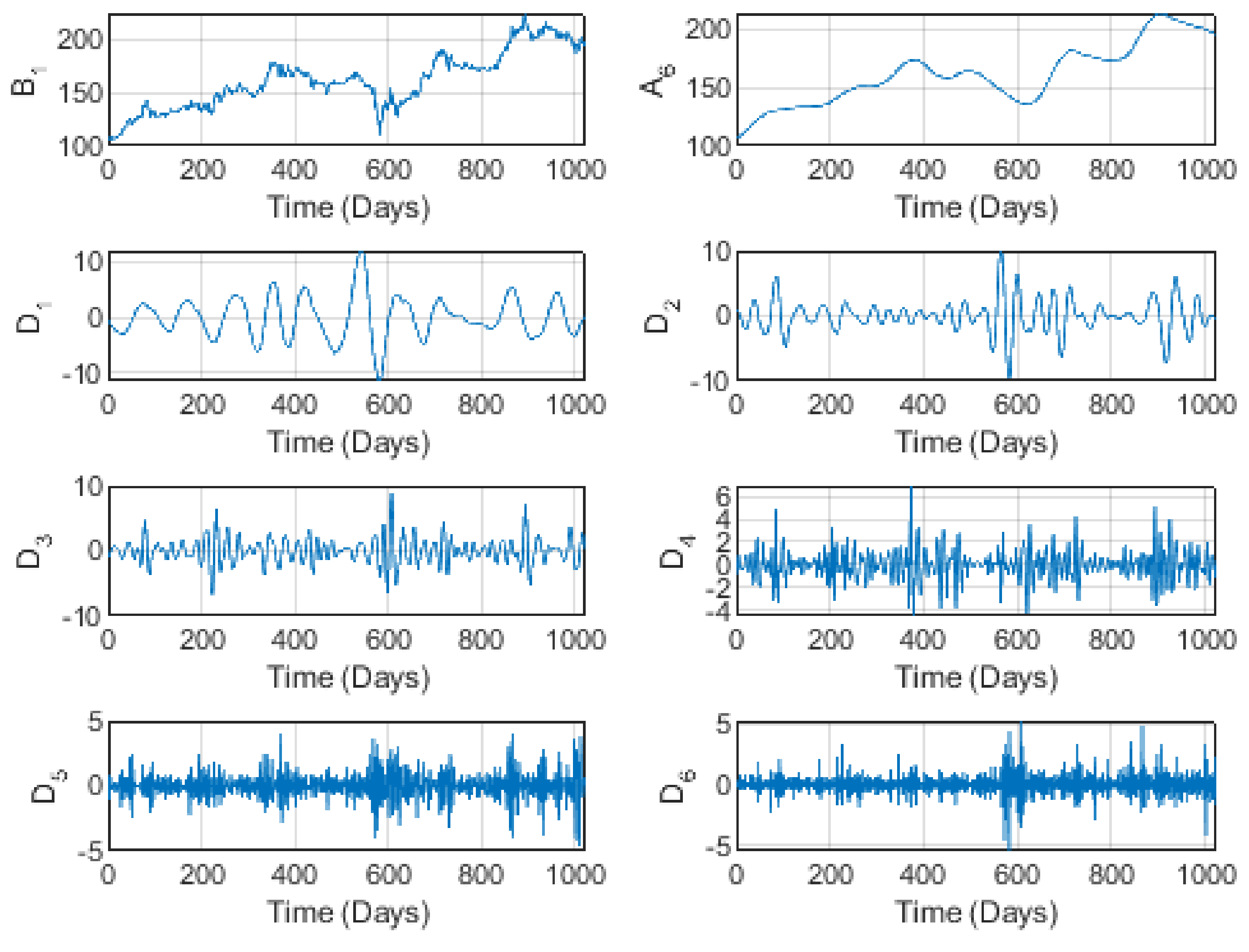
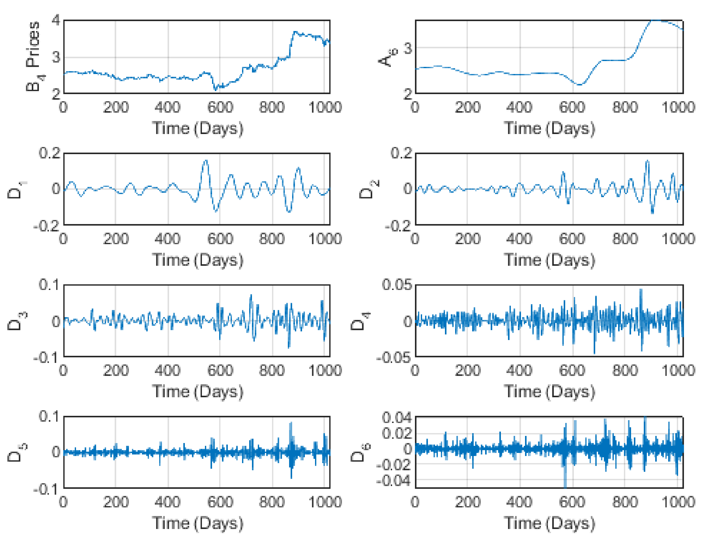
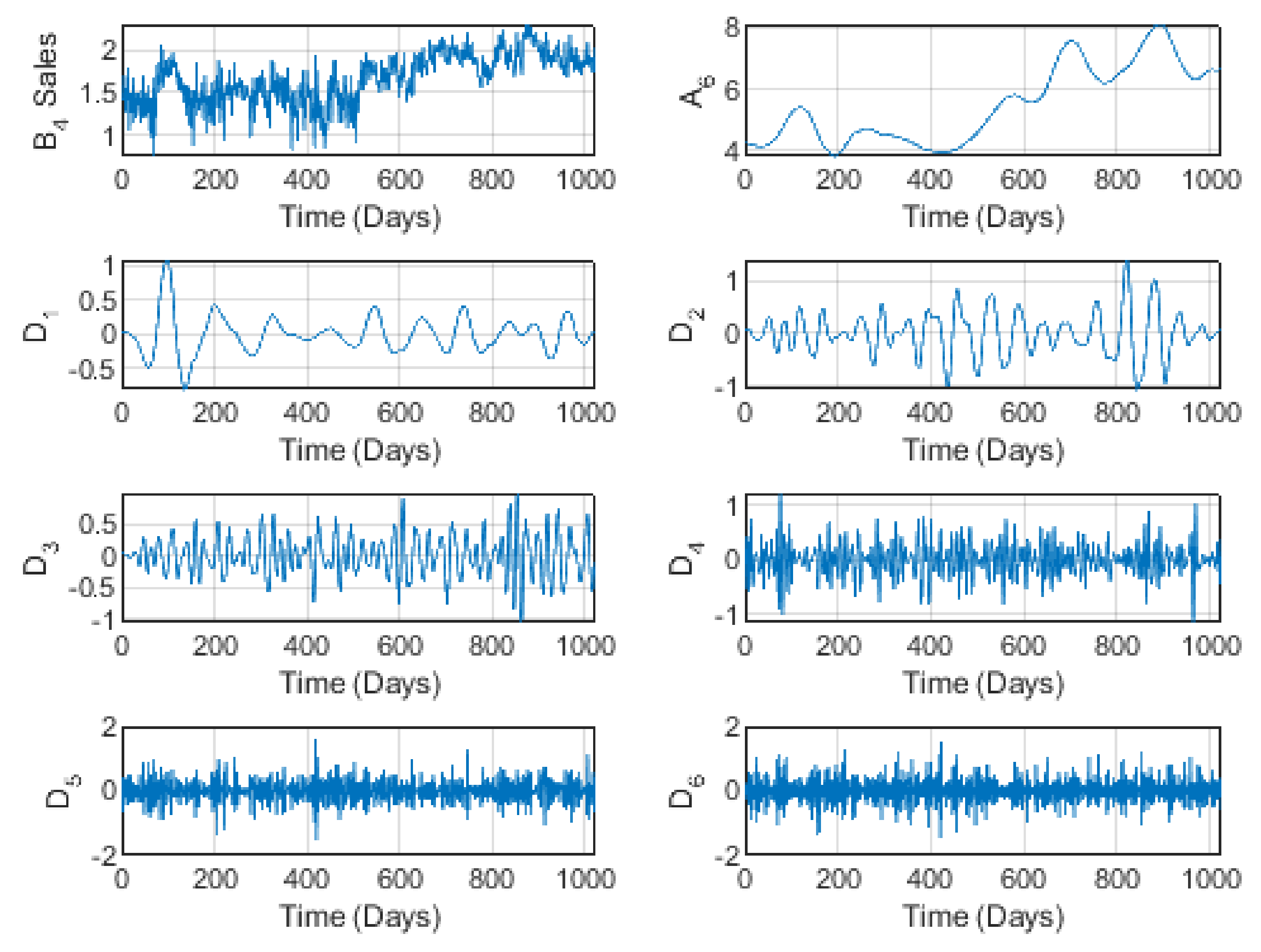
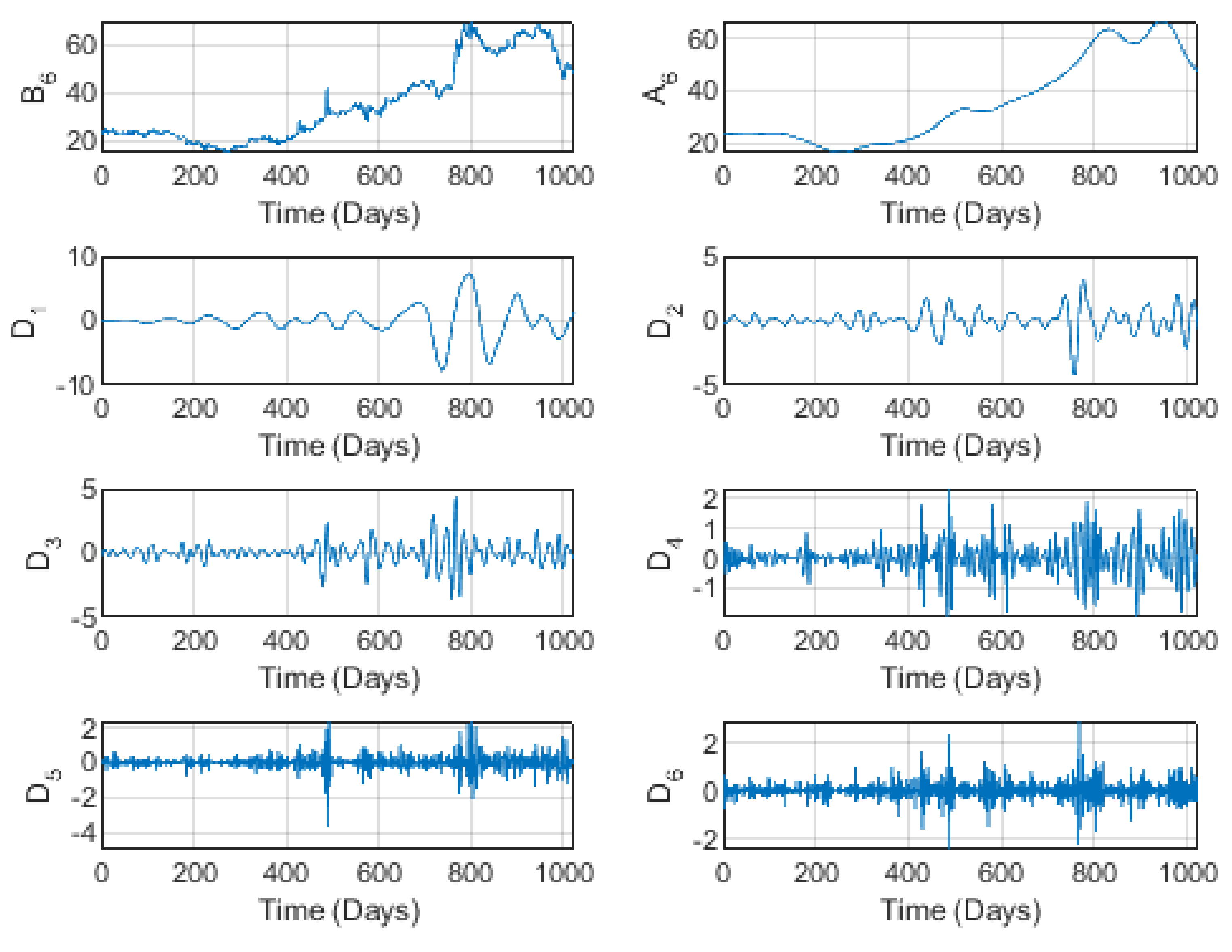
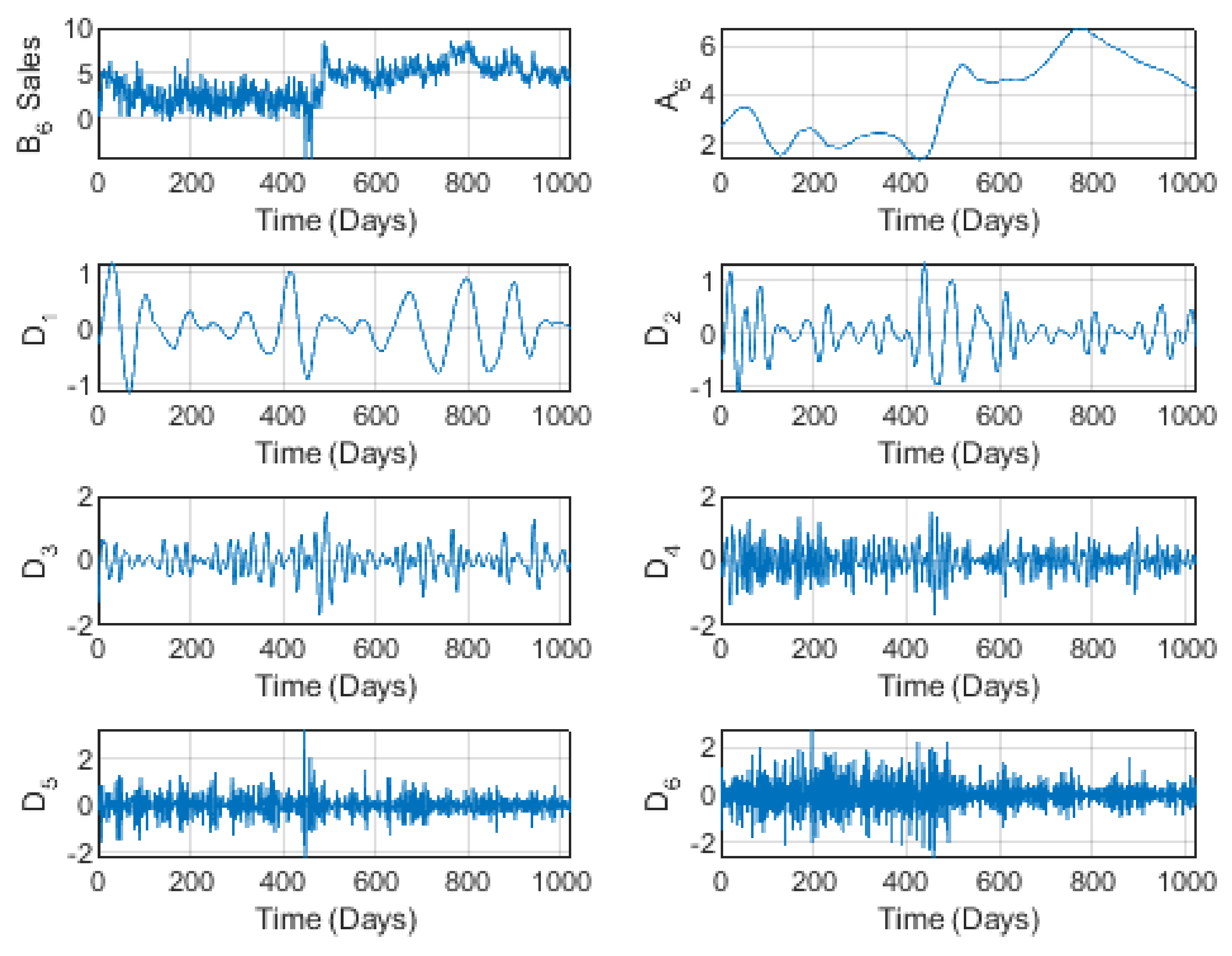
Figure 1, illustrating the wavelet decomposition of $B_1$ prices, shows a somewhat increasing behavior, clearly illustrated by the level 6 trend $A_6$, reminiscent of some perturbations at medium-to-long scales. However, the trend shows no cycles (periodic behavior) for the $B_1$ prices. The perturbation is confirmed in the detail components $D_1$ to $D_6$. According to $D_1,D_2$ a certain pseudo-periodicity seems to take place, with some differences in the maximum prices. This may be explained by the fact that at short time scales (such as weeks in the classical treatments of the time factor), prices are influenced by competitors on the one hand and the global behavior of the market (national as well as international) on the other. One essential factor to be considered is the COVID-19 pandemic, which covered a great part of the period of study and which certainly resulted in decreased sales so that, to compensate for the quantities in stock and thus to recover losses, the company had to increase prices, as in many other cases. This fact is easily shown in the $B_1$ sales graphs in Figure 2, where we clearly observe an upward trend in sales whenever prices decreased and a downward trend in sales whenever prices increased. In addition, both prices and sales are volatile at long time scales, according to the detail components $D_3$ to $D_6$. We may thus conclude for this brand that short time scales are more comprehensive and easy to understand for consumers, investors, and managers.

Figure 1. The wavelet decomposition of the Jarir brand $B_1$ prices at level 6.

Figure 1. The wavelet decomposition of the Jarir brand $B_1$ prices at level 6.

Figure 2. The wavelet decomposition of the Jarir brand $B_1$ sales at level 6.

Figure 2. The wavelet decomposition of the Jarir brand $B_1$ sales at level 6.

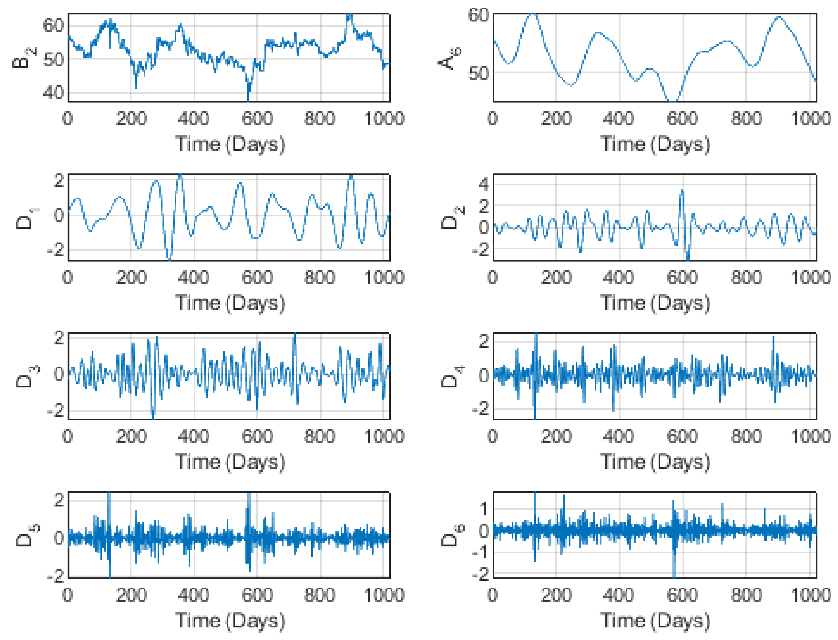
In Figure 3, there is a slight variation around the mean (median), with no exact periodicity but instead a slight pseudo-periodic structure. This behavior is repeated in the sales illustrated in Figure 4. However, some anomalies appear, essentially at all time scales. This behavior can be naturally understood from the fact that Almarai is a completely national company, based on completely national products. Therefore, compared to $B_1$, for example, its prices and volumes are not strongly affected by importation. In addition, its products are the oldest, the best in the market (according to the majority of consumers), and are consumed daily. All these factors allow price stability in the market, despite a slight growth in the volume of production. In addition, prices and sales seem to reflect the same behavior at short and long time scales. These fluctuations are clearly illustrated by the detail components $D_1$ to $D_6$. Nevertheless, slight fluctuations remain around the mean for all the time scales.

Figure 3. The wavelet decomposition of the Almarai brand $B_2$ prices at level 6.

Figure 3. The wavelet decomposition of the Almarai brand $B_2$ prices at level 6.

Figure 4. The wavelet decomposition of the Almarai brand $B_2$ sales at level 6.

Figure 4. The wavelet decomposition of the Almarai brand $B_2$ sales at level 6.

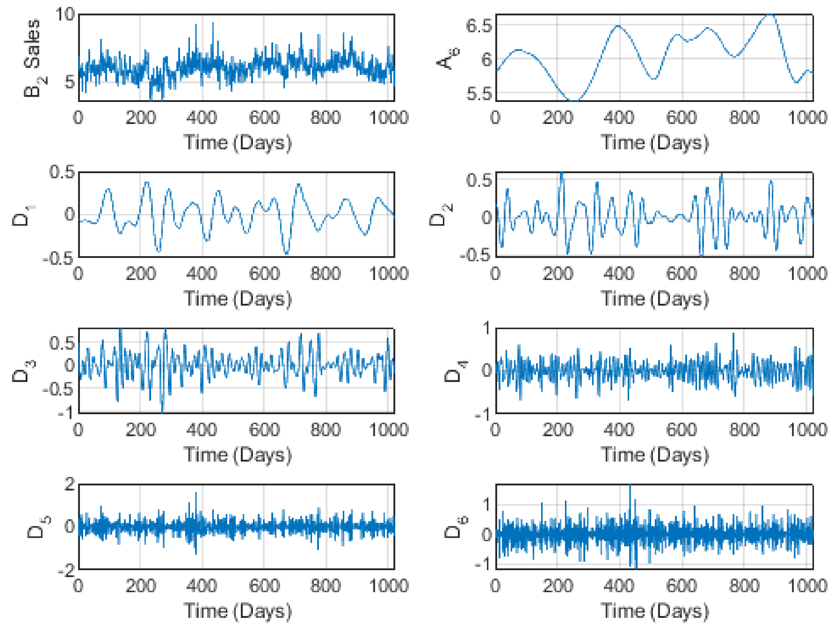
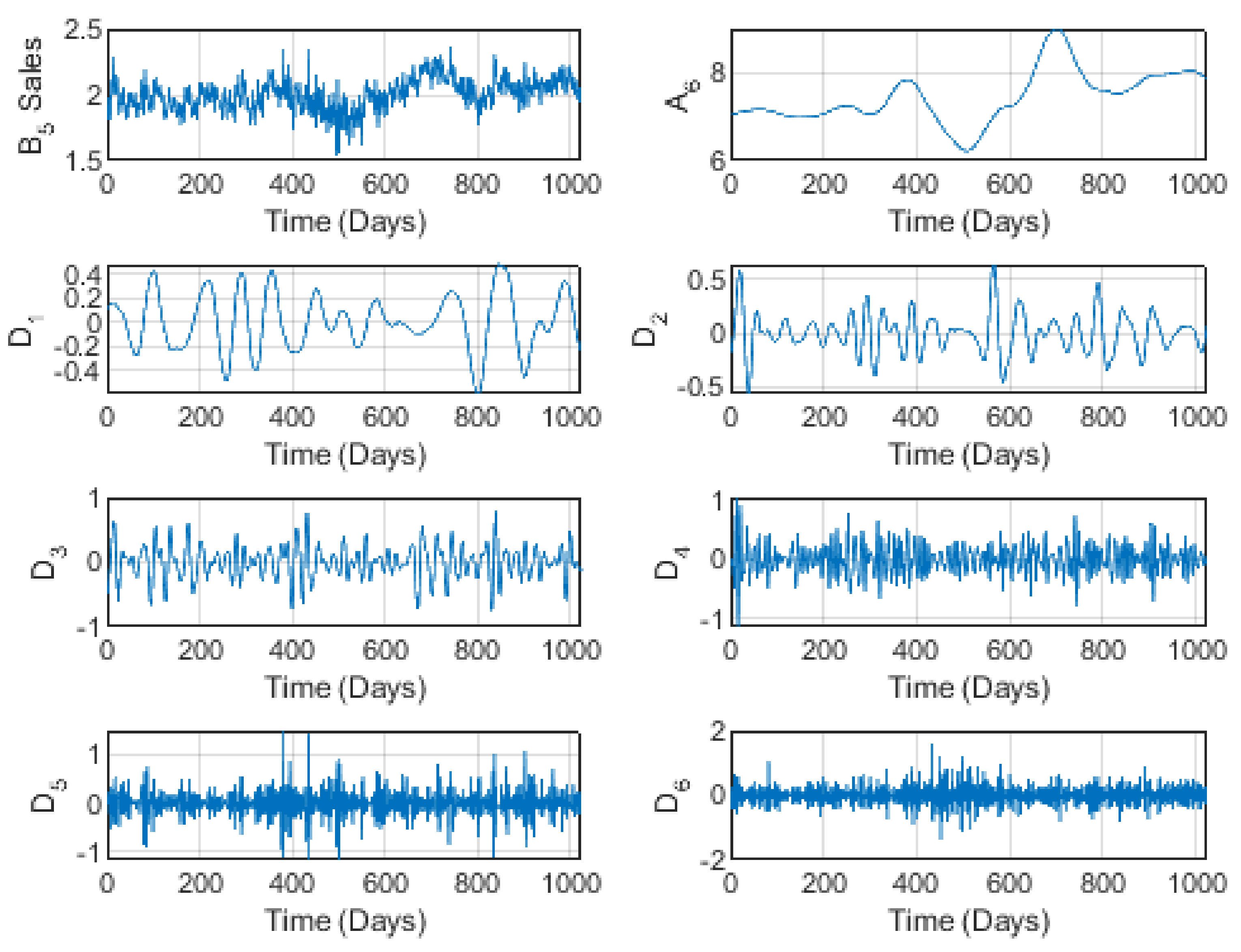
Figure 5 and Figure 6 illustrate the behavior of the brand $B_3$ prices and sales for level 6 wavelet decomposition. Here also, we notice a global increase in both series, which is clearly shown in the trend $A_6$. This increase is sometimes interspersed with small fluctuations. This brand is one of the major suppliers of communications needs in the entire Kingdom of Saudi Arabia. During the COVID-19 quarantine period, STC sales grew (seen clearly in $A_6$) due to the increase in remote and/or distance communications in almost all domains. Nevertheless, we notice some pseudo-periodicity at short time scales.

Figure 5. The wavelet decomposition of the STC brand $B_3$ prices at level 4.

Figure 5. The wavelet decomposition of the STC brand $B_3$ prices at level 4.

Figure 6. The wavelet decomposition of the STC brand $B_3$ sales at level 4.

Figure 6. The wavelet decomposition of the STC brand $B_3$ sales at level 4.

Figure 7 and Figure 8 show quasi-stability at short and medium time scales, followed by a global increase at higher horizons. This increase may also be due to high consumer demand as an alternative during the quarantine period for COVID-19. The pseudo-periodicity and stability appearing at short and medium horizons effectively breaks down at long time scales for these reasons. Moreover, with the lack of importation of similar products, consumers turned to national brands, contributing to the increase in sales and consequently in prices. On the other hand, a high proportion of these types of sales are imported (as raw or elementary commodities). Therefore, with the economic recession afflicting the market for the long COVID-19 period, merchants had to increase prices to compensate for a part of their losses. In addition, other companies use many of the products of this brand, such as polyester and nylon. In critical periods such as during COVID-19, it is necessary to use national stocks. This induces an increase in both sales and prices.

Figure 7. The wavelet decomposition of the Al Abdullatif brand $B_4$ prices at level 6.

Figure 7. The wavelet decomposition of the Al Abdullatif brand $B_4$ prices at level 6.

Figure 8. The wavelet decomposition of the Al Abdullatif brand $B_4$ sales at level 6.

Figure 8. The wavelet decomposition of the Al Abdullatif brand $B_4$ sales at level 6.

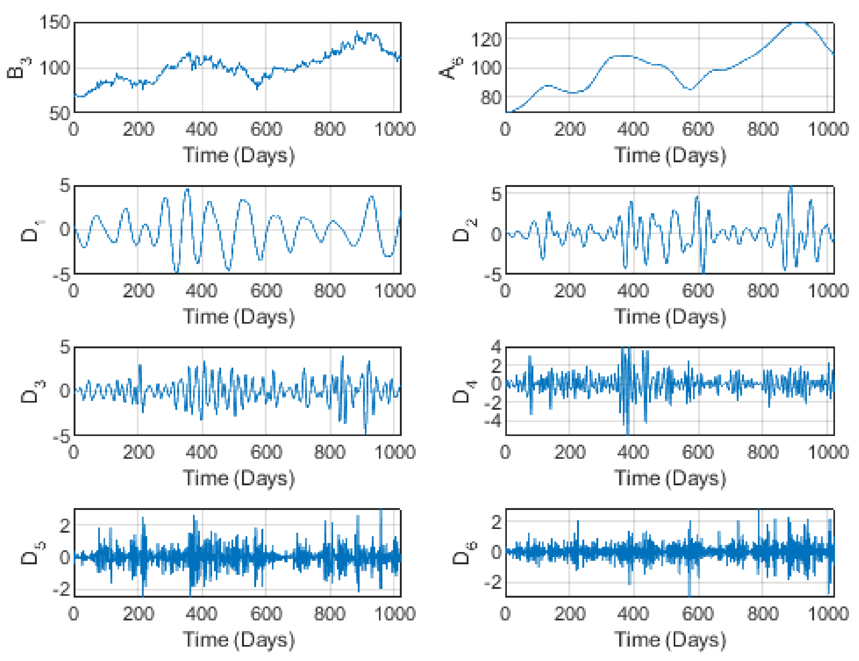
The brand $B_5$, illustrated by Figure 9 and Figure 10 for prices and sales, respectively, is characterized by a small skewness and kurtosis and quite a small Std. This indicates some stability in both prices and sales, showing some small fluctuations but no important extreme values. As its trend $A_6$ indicates, prices started to decrease at short time scales, turning to an increase at high horizons, with a slow increase at medium levels. Sales seemed to be stable globally at short horizons, decreasing at medium levels, and increasing at longer time scales. Recall that EIC is a national manufacturer of electric instruments. Such instruments need many raw materials, mainly imported from outside the kingdom. Therefore, considering the COVID-19 situation, and with the orientation towards encouraging national and local industry and production being one of the main goals of the Vision 2030 program, these companies have experienced expansion and development in the volumes of sales, as well as in prices. Nevertheless, the graphical representations of the detail components do not reflect any cycles, as might be expected in classical studies.

Figure 11 and Figure 12 illustrate the time-scale behavior of brand $B_6$ prices and sales, according to the wavelet decomposition at level $J-6$. A global increase in both prices and sales can clearly be seen, especially at longer time scales. By investigating the detail components $D_1$ to $D_6$, we may easily exclude the idea of cycles for this series, especially for low/medium horizons. At longer time scales, the series becomes more and more volatile, as for the preceding brands. The increase at the higher horizons is due to the orientation of consumers to local/national products, as there was no importation from outside. Moreover, this brand specializes mainly in national clothing, representing a style that is not widely known outside the GCC countries, although some companies in China target the GCC market. These outside companies discontinued their exports during the COVID-19 period, which therefore resulted in increased sales of national clothing products. In addition, due to the Vision 2030 program, these local/national brands and the producing companies are forced to implement government directions and guidelines to develop and expand national production.

Figure 9. The wavelet decomposition of the EIC brand $B_5$ prices at level 6.

Figure 9. The wavelet decomposition of the EIC brand $B_5$ prices at level 6.

Figure 10. The wavelet decomposition of the EIC brand $B_5$ sales at level 6.

Figure 10. The wavelet decomposition of the EIC brand $B_5$ sales at level 6.

Figure 11. The wavelet decomposition of the Al Aseel brand $B_6$ prices at level 6.

Figure 11. The wavelet decomposition of the Al Aseel brand $B_6$ prices at level 6.

Figure 12. The wavelet decomposition of the Al Aseel brand $B_6$ sales at level 6.

Figure 12. The wavelet decomposition of the Al Aseel brand $B_6$ sales at level 6.

Overall, these graphs, especially their detail components, reduce the ideas of cycles and stationarity for these marketing series and show instead a volatile behavior, which increases with the time scale. This indicates that the market concerned is emergent, and economic laws must be applied carefully by investors and managers. These facts may have many reasons. One is the COVID-19 crisis, which has been positively used in some cases, especially regarding telecommunications supplies and national products including foods (Almarai) and clothing (Al Aseel). However, this was a disadvantageous situation for many brands relying on imported raw materials, such as EIC. In addition, there was an effect of labor resettlement, which resulted in a considerable amount of non-highly-qualified labor in many sectors. This fact, although it constitutes a principal goal in the Vision 2030 program, may have reduced productivity.

We consider that more investigation into this volatile movement should be performed by improving tools such as the implementation of stochastic factors in the model and/or experimentation with non-uniform time-scale models, as in [13].

In the remainder of the paper, we focus on the validation of the mathematical model (9). For this purpose, we consider different cases of competitors of the brands applied, as illustrated in

Table 4. Some main competitors of brands $B_1$, $B_2$, and $B_3$.

Brands	Top Competitor(s)
$B_1$—Jarir Bookstore	Alobeikan ($CP{B}_1$)
$B_2$—Almarai	Nadec ($CP{B}_2$)
$B_3$—STC	Zain ($CP{B}_3$)

. We recall that all these brands are distributed throughout the whole kingdom in all the provinces, and they are also offered via an online purchase and delivery service throughout the kingdom. This gives them the same opportunities for the distribution of their sales or products at all times and places. This was confirmed numerically, as the numerical experiments showed that $7.28\times {10}^{-12}\le {\beta }_3\le 1.2\times {10}^{-9}$ and ${\beta }_4=0$.

In

Table 5. Model (9) coefficient estimations for brands $B_i$, $1\le i\le 6$, at different levels.

Coefficient	Model (8)	${\mathit{A}}_6$	Level 1	Level 2	Level 3	Level 4	Level 5	Level 6
The brand $B_1$
${\beta }_0$	$-95.21$	$-167.57$	$-0.01$	$0.01$	$-0.01$	$-0.02$	$-0.09$	$-0.24$
${\beta }_1$	$1.93$	$2.45$	$1.27$	$12.75$	$4.55$	$2.85$	$-7.13$	$-4.82$
${\beta }_2$	$-6.05$	$-7.21$	$-10.78$	$-8.27$	$15.78$	$-24.60$	$-3.54$	$-12.48$
The brand $B_2$
${\beta }_0$	$-42.76$	$-131.92$	$-0.06$	$0.02$	$-0.002$	$-0.42$	$0.21$	$1.10$
${\beta }_1$	$10.31$	$12.98$	$227.21$	$166.02$	$-10.61$	$45.20$	$-6.22$	$-34.84$
${\beta }_2$	$2.17$	$0.31$	$53.16$	$-72.86$	$-14.65$	$60.14$	$-6.97$	$23.62$
The brand $B_3$
${\beta }_0$	$139.14$	$72.38$	$-0.006$	$-0.45$	$-0.82$	$-14.90$	$35.88$	$21.80$
${\beta }_1$	$-5.91$	$-7.47$	$-590.90$	$80.18$	$-314.70$	$41.34$	$01.99$	$16.75$
${\beta }_2$	$122.77$	$139.51$	$2436.79$	$-396.59$	$351.10$	$-394.74$	$-980$	$-167.01$

, we provide the estimations of the coefficients of models (8) and (9), using the usual ordinary least squares (OLS) estimates for the linear regression coefficients of the variable $S_{t,j}$ on the variables $P_{t,j}$, $C{P}_{t,j}$, $P{R}_{t,j}$, and $D_{t,j}$ in model (9). More precisely, the column named Model (8) gives the estimations of the coefficients ${\beta }_i$, $i=1,2,3$, for the original non-wavelet model (8). The column $A_6$ in Table 5 shows the estimations of the coefficients of model (9) when projected on the approximation space $V_6$. The columns named Level i, $1\le i\le 6$ show the estimations of the coefficients of model (9) when projected on the detail space $W_i$, $1\le i\le 6$.

In addition, to further investigate the models applied here and to eliminate the descriptive statistics context, we provide in

Table 6. Confidence intervals at $95\%$ for model (9) coefficient estimations for brands $B_i$, $1\le i\le 6$, at different levels.

Coeff	Model (8)	${\mathit{A}}_6$	Level 1	Level 2	Level 3	Level 4	Level 5	Level 6
The brand $B_1$
${\beta }_0$	[−96.24; −95.18]	[−168.60; −165.53]	[−0.04; 0.02]	[−0.02; 0.04]	[−0.04; 0.02]	[−0.05; 0.02]	[−0.12; −0.08]	[−0.27; −0.21]
${\beta }_1$	[1.89; 1.96]	[2.41; 2.48]	[1.23; 1.30]	[12.71; 12.78]	[4.51; 4.58]	[2.81; 2.88]	[−7.16; −7.09]	[−4.85; −4.78]
${\beta }_2$	[−6.11; −6.00]	[−7.27; −7.16]	[−10.84; −10.73]	[−8.33; −8.22]	[15.71; 15.82]	[−24.66; −24.55]	[−3.60; −3.49]	[−12.54; −12.43]
The brand $B_2$
${\beta }_0$	[−43.79; −42.77]	[−132.95; −130.88]	[−0.19; 0.02]	[−0.11; 0.05]	[−0.03; 0.02]	[−0.55; −0.30]	[0.10; 0.30]	[1.01; 1.23]
${\beta }_1$	[10.27; 10.34]	[12.94; 13.01]	[227.17; 227.24]	[165.98; 166.05]	[−10.64; −10.57]	[45.16; 45.23]	[−6.25; −6.18]	[−34.87; −34.80]
${\beta }_2$	[2.10; 2.22]	[0.24; 0.36]	[53.09; 53.21]	[−72.92; −72.80]	[−14.71; −14.59]	[60.07; 60.19]	[−7.03; −6.91]	[23.55; 23.67]
The brand $B_3$
${\beta }_0$	[139.10; 139.17]	[72.34; 72.41]	[−0.03; 0.02]	[−0.48; −0.41]	[−0.85; −0.78]	[−14.93; −14.86]	[35.84; 35.91]	[21.76; 21.83]
${\beta }_1$	[−5.94; −5.87]	[−7.50; −7.43]	[−590.93; −590.86]	[80.14; 80.21]	[−314.73; −314.66]	[41.30; 41.37]	[1.95; 2.02]	[16.71; 16.78]
${\beta }_2$	[122.70; 122.81]	[139.44; 139.55]	[2436.72; 2436.83]	[−396.65; −396.54]	[351.03; 351.14]	[−394.80; −394.69]	[−980.06; −979.95]	[−167.07; −166.96]

some inference statistics results based on confidence intervals for each coefficient estimated previously in Table 5. More precisely, for a series $Z_i$, $i=,\dots ,N$ ($N\in \mathbb{N}$ being the size of the series), the mean is computed as

$${\displaystyle \overline{Z}={\displaystyle \frac{1}{N}}\sum _{i=1}^N{Z}_i.}$$

Next, the standard deviation is evaluated as

$${\sigma }_Z=\sqrt{{\displaystyle {\displaystyle \frac{1}{N-1}}\sum _{i=1}^N{(Z_i-\overline{Z})}^2}}.$$

The confidence intervals are deduced as

$$\left[\overline{Z}-t_{N-1;0.975}{\displaystyle \frac{Z}{\sqrt{N}}},\overline{Z}+t_{N-1;0.975}{\displaystyle \frac{Z}{\sqrt{N}}}\right],$$

In

Table 7. Residue for model (8) and (9) estimates at different levels.

Brand	Model (8)	${\mathit{A}}_6$	Level 1	Level 2	Level 3	Level 4	Level 5	Level 6
$B_1$	0.26	0.58	0.17	0.12	0.78	0.55	0.56	0.23
$B_2$	0.68	0.19	0.40	0.33	0.23	0.21	0.18	0.10
$B_3$	0.39	0.63	0.30	0.14	0.12	0.99	0.65	0.23

, we provide further inferential statistics such as the residue due to the estimations of the coefficients in models (8) and (9), where the residue is estimated for an observed variable Y and its empirical value $\widehat{Y}$ by $Y-\widehat{Y}$. In Table 7, we provide precisely the standard deviation associated with the residue, as

$$Residue=\sqrt{{\displaystyle \frac{\parallel Y-\widehat{Y}{\parallel }_2^2}{N-2}}},$$

where N is the size of the vector Y, and for a vector $u\in {\mathbb{R}}^N$, ${\parallel u\parallel }_2$, stands for its usual Euclidean norm.

Table 5 shows an important influence of the prices for both the original non-wavelet model (8) and the wavelet time-scale model ((9), reflected in the values of the coefficient ${\beta }_1$. For the brand $B_1$, for example, this coefficient is globally important in the approximation component $A_6$, which describes the general behavior (trend) of the time series. By considering the microscopic scale, we notice that this coefficient reflects a strong influence over a short horizon (level 1) on the sales, and the influence becomes greater at medium-to-high horizons (level 2, level 3, level 4, level 5, and level 6), even becoming negative at very long time scales. The competitor price, however, negatively influences the model and is estimated by the negative coefficient ${\beta }_2$, except at the medium level $L3$, where an increase or an extreme value appears. An even greater effect exists for higher horizons.

The same interpretations can also be made for the brands $B_2$ and $B_3$, where both the prices and the competitor prices reflect important influences expressed by means of the high coefficients ${\beta }_1$ and ${\beta }_2$. For the brand $B_2$, we notice higher positive influences at short time scales for ${\beta }_1$, followed by a reduction at the medium level $L3$, becoming higher but negative for the long-term horizons. Nevertheless, the prices are globally positively influenced.

In addition, null values for ${\beta }_4$ suggest that there is no influence of the variable $D_t$. This is natural for the Saudi market, especially for national brands. Indeed, all the chosen brands and their associated sales companies own collection centers, warehouses and distribution points throughout the kingdom. In addition, there are e-sales and delivery services available in all the emirates, as well as all the governorates in the kingdom, even in small cities and villages. This means that distribution is not the subject of great competition between the firms. During the COVID-19 quarantine period, the state was keen to support companies to distribute their products throughout the country. Furthermore, in relation to the Vision 2030 program, the state plans to provide the same opportunities for national companies, to encourage production as well as investment in national brands and competition. This will have an important effect on the economy and on society, as it will provide jobs in the national labor market, thus affecting quality of life and well-being in society from the economic point of view.

The promotional coefficient ${\beta }_3$ also has a small value (almost null) which suggests that the promotion factor does not greatly influence the movements of prices and sales. This finding is also reasonable in KSA, as all these top brands apply promotional prices throughout the whole year. Every week, promotions of different products under the same brand are announced. This is also an important point, as it leads to a increase in sales and thus influences sales especially.

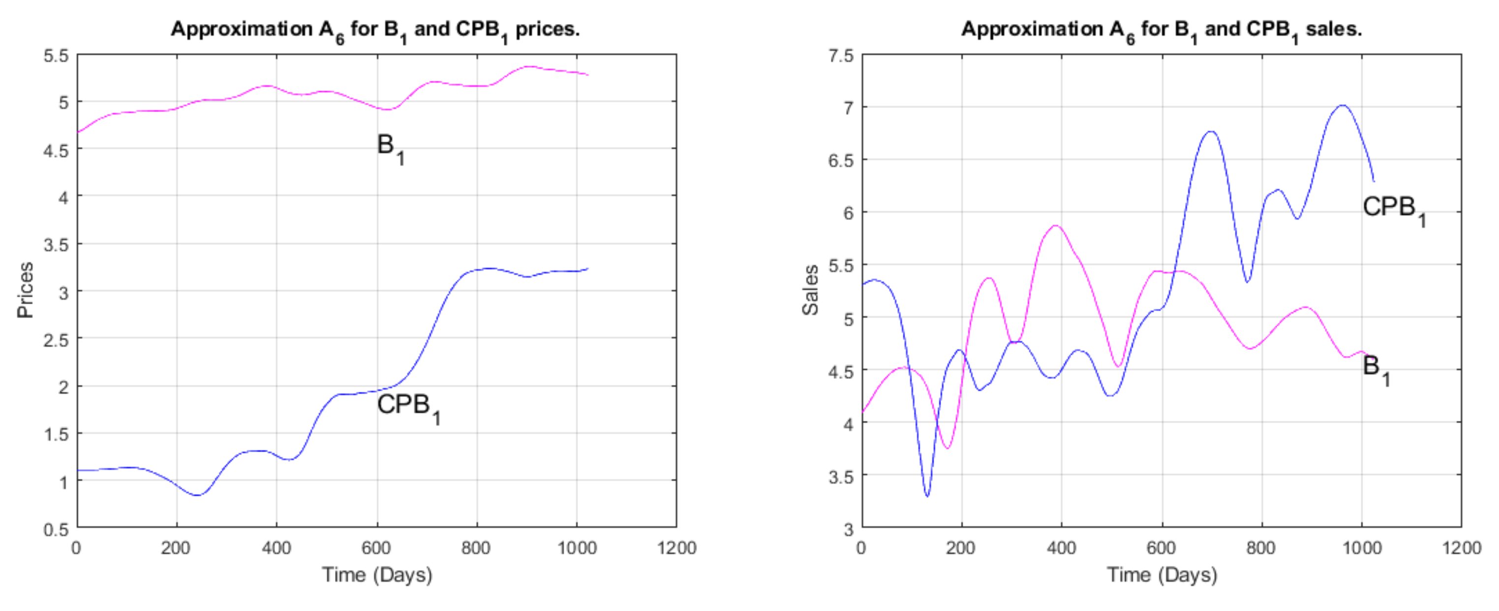
In Figure 13, Figure 14 and Figure 15, comparisons between the brand prices and sales for $B_1$, $B_2$, and $B_3$ and those of their competitor brands $CP{B}_1$, $CP{B}_2$, and $CP{B}_3$, respectively, are illustrated graphically at the maximum level of wavelet decomposition $J=6$, by means of the filtered prices.

These last figures are in complete agreement with the results previously discussed, especially those in Table 3. Indeed, we notice from Figure 13 that the variations in the $B_1$ prices and sales are ahead of those of its competitor $CP{B}_1$. Prices and sales for both of them show a global increase, with higher $B_1$ prices. However, the sales also show some oscillations, with higher competitor sales at the longer time scales. This may be explained by the fact that $B_1$ sales are in fact imported products from outside the kingdom, except for a few types of products. However, the competitor, Alobeikan, mainly focuses on a national printing press concerned with printing books internally, or at least those imported and distributed within GCC countries. This meant that its sales increased during the COVID-19 period, which here represents the long-term horizons.

Figure 13. The wavelet approximation $A_6$ for $B_1$ and $CP{B}_1$ prices and sales at level 6.

Figure 13. The wavelet approximation $A_6$ for $B_1$ and $CP{B}_1$ prices and sales at level 6.

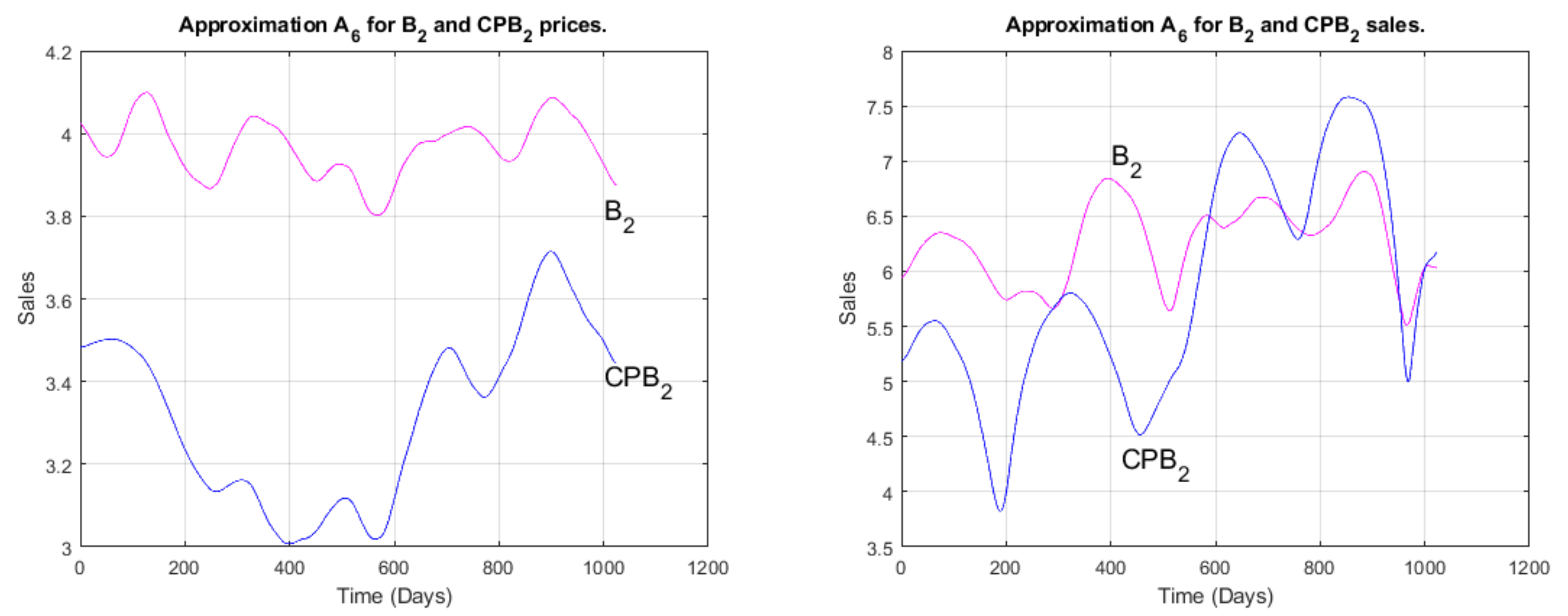
The brand $B_2$ and its competitor $CP{B}_2$ are both concerned with national foods, and thus were not widely influenced by the COVID-19 pandemic as they already used internal products. Nevertheless, the dominance of the brand $B_1$ sales and prices is clearly illustrated in Figure 14. This is also compatible with Table 3, where the corresponding coefficient ${\beta }_2$ is globally positive, although low for $A_6$, and perturbed (oscillating between positive and negative values) for some medium-to-long time scales.

Figure 14. The wavelet approximations $A_6$ for $B_2$ and $CP{B}_2$ prices and sales at level 6.

Figure 14. The wavelet approximations $A_6$ for $B_2$ and $CP{B}_2$ prices and sales at level 6.

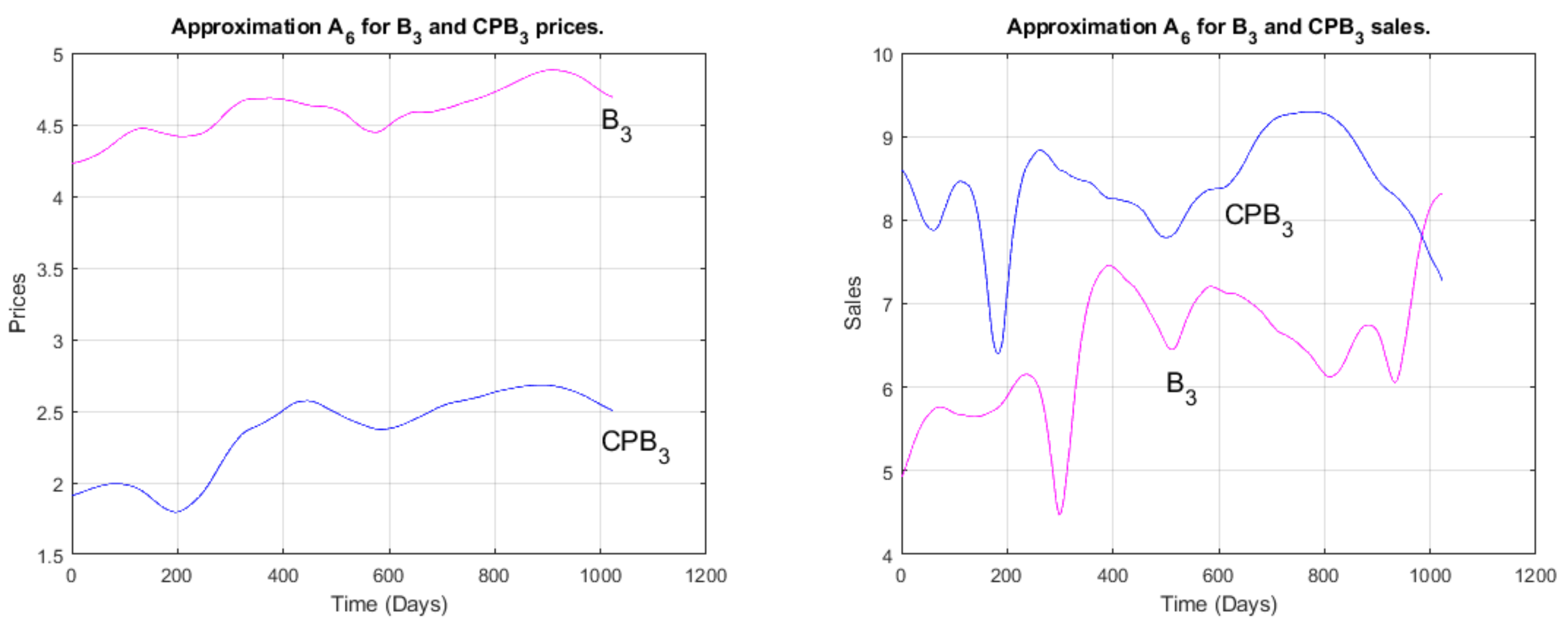
Figure 15 reflects the variation in sales/prices for the brand $B_3$ and its competitor $CP{B}_3$. We can easily observe the dominance (superiority) of the prices of the brand $B_3$ compared to its competitor’s prices. However, this dominance may itself be the cause of the reversed order from the point of view of sales, where the competitor shows a superiority in the market. This may be due to the demand for the products of the second brand, as its prices are within the reach of middle-income consumers, regardless of the quality of the product. We recall that a large segment of the population is made up of foreign workers whose wages are low compared to those of citizens, and this dominant group tends to require cheaper prices for daily consumption. It should also be noted that the first label focuses on the traditional national dress of citizens more than on other types of clothing.

Figure 15. The wavelet approximation $A_6$ for $B_3$ and $CP{B}_3$ prices and sales at level 6.

Figure 15. The wavelet approximation $A_6$ for $B_3$ and $CP{B}_3$ prices and sales at level 6.

Economically speaking, the results are of great importance. From a theoretical point of view, they confirm the presence of the time-scale factor or behavior in marketing time series, and thus can lead scientists in the field to take this factor into consideration in future models. From a practical point of view, or considering economic and financial reality, the results clearly indicate the movements of the markets studied. We notice a stability at short time scales, with a slight growth for many brands. Then, the volumes and the prices become disturbed for medium horizons, sometimes with large fluctuations. Finally, for long horizons (high levels), we notice a remarkable increase. These facts can be justified and explained economically. Indeed, the study period is strongly related to several sociological and political phenomena which had a great influence on the economic state of the market. At the beginning of the period, the local market was affected by the turmoil in several Arab countries, which negatively affected sales, especially since a large part of the workforce originally belonged to these countries. The Qatar embargo and the wars that broke out near the kingdom (forcing it to be involved in some of them) had a great impact on marketing. Thus, the local market lost several tributaries and extensions.

The beginning of the period of study also coincided with the discussion about the added tax on all sales, which negatively affected the purchasing power of citizens and residents and led to a kind of stagnation in the market. Furthermore, some severe laws relating to residents, such as taxes on family members, also led to the permanent deportation of a large number of residents and their families in their countries of origin. This factor had the greatest impact on sales and commercial movements.

As a result of this stagnation, the authorities resorted to ways to compensate for the added value through grants to employees and support for national production, which paralleled the idea of reducing the dependence on oil as a sole income, instead encouraging national industries, of which commercial sales represent a large part. This slowdown contributed to the return of market movements in general and led to an increase in the volume of sales, which in turn led to a recovery in prices. All this coincided with some stability in some Arab Spring countries and the return of normal Gulf relations.

The last factor that should be noted concerns the stability of the local and global situation regarding the COVID-19 pandemic, which has now been brought under control. This led to the reopening of the holy cities (Makkah and Madina) to visitors from all over the world and the return of the labor force to its activities. We recall that the holy cities have the largest human gatherings in the world and are therefore the largest promoters and consumers of national sales, with a significant effect on distribution and publicity for various brands outside the Kingdom of Saudi Arabia.

6. Conclusions

In many applications of time series, such as in marketing, classical studies suggest non-stationarity and short time scales. Nevertheless, studies confirm the existence of a time–frequency aspect. Many mathematical tools and models have been applied by researchers to explain the time-scale behavior of marketing series. Wavelets are the most recent and most powerful tool for this purpose, due to their ability to explain both the time and frequency dependencies in the time series.

In the present work, we aimed to study the time-scale impact by applying wavelets and their supports instead of the classical methods based on classical periods usually applied in the fields of marketing, economics, finance, etc. These periods are always expressed as weeks, months, or years.

Wavelets were therefore exploited to improve marketing models by projecting such models on different horizons via wavelet processing. These horizons reflected the time scales, and permitted detailed observation of the situation with respect to brand prices and sales in Saudi Arabia, one of the largest economies in the world. The findings showed that the wavelet time-scale models effectively permitted a good understanding of brand movements, especially during crises such as the last pandemic, and in view of economic and political plans such as Vision 2030.

Although our main aim in the present work was to point out the influence of time-scale modeling on marketing models, rather than undertaking a pure statistical analysis of the model itself, important features such as autocorrelation and heteroscedasticity were identified. Recall that in classical methods, the confidence intervals, for example, use statistics that are the same for the whole model. However, in the present study, the different time-scale versions of the model induced variable statistics. This confirmed that the confidence interval bounds depend strongly on the fluctuations and that these fluctuations are not due to seasonal oscillations (which may be left in the series). This was also confirmed by the approximation components resulting from the wavelet decomposition, where non-periodic phenomena appeared clearly.

Otherwise, the presence of heteroscedasticity does not in fact induce bias in the results, but it instead may bias the standard deviations obtained via OLS. To investigate this, we may regress the square of the residuals on the exogenous (dependent) variables of the original regression and test if the coefficients are jointly significant. These results (partially omitted here) may be considered as limitations of the time-scale models proposed, and a future research direction may involve improvements via suitable transformations on the model or the data, to identify more features such as heteroscedasticity.

Nevertheless, the present study showed that even the wavelet time-scale models may be improved, and many hidden structures may be discovered by involving more tools. For the moment, we suggest including random and/or non-uniform wavelets and time scales to extend the existing models.

Sophisticated models will provide marketing managers such as investors and analysts with necessary and useful information to assist their decisions and analyses.