Adaptive Sliding Mode Control via Backstepping for an Air-Breathing Hypersonic Vehicle Using a Double Power Reaching Law

Abstract

This paper presents a backstepping-based adaptive sliding mode control scheme using a new double power reaching law for an air-breathing hypersonic vehicle (AHV) with uncertainties. A novel double power reaching law is proposed to speed up the state stabilization. A backstepping control scheme is proposed for a class of high-order nonlinear system with uncertainties. Then, a novel sliding mode controller using the new double power reaching law is developed to maintain the high tracking performance of the AHV. In order to further attenuate the influence of uncertainties, new adaptive laws are employed. Lastly, simulation studies show that the novel double power reaching law can guarantee that the state of the system converges to zero equilibrium in fixed time, and the controller proposed can effectively reduce the influence of uncertainties on the AHV and achieve good tracking performance.

1. Introduction

An air-breathing hypersonic vehicle (AHV) refers to a scramjet-powered vehicle that can fly at speeds of more than Mach 5 [1,2,3]. AHVs are of great civilian and military value because of their high Mach numbers, high altitude range, and the characteristic of prompt global response. Therefore, AHVs have always been a hot topic in aviation technology research [4,5,6]. However, it is a great challenge to design a high-performance flight control system, due to AHVs with high couplings, strong nonlinearities, and strong uncertainties [7,8].

The model of an AHV has great uncertainties for the following reasons. Firstly, because of the high speed of the AHV, aerodynamic parameters of aircraft are difficult to capture accurately. Secondly, due to the large flight envelope of the AHV, it is difficult to accurately estimate atmospheric properties and aerodynamic characteristics. In addition, the insufficient data of the flight test also make AHV models inaccurate. Therefore, the design of a robust controller is particularly important for AHV technology. Currently, there are many methods used to study the uncertainties and nonlinearity of AHV in the literature, such as H∞ [9,10], fuzzy control [11,12,13], neural network control [14,15,16], sliding mode control [17,18,19,20], backstepping control [21,22,23,24], and adaptive control [25,26,27,28].

Recently, backstepping has been widely used in nonlinear systems. In the process of design, backstepping decomposes a complex high-order nonlinear system into multiple low-order subsystems, and designs a separate Lyapunov function for each subsystem. These features of backstepping make it less difficult to design high-order control systems, so it is increasingly applied to the design of AHV controllers [29]. For instance, a robust, adaptive backstepping control scheme was designed for the flexible AHV with input restriction and aerodynamic uncertainties by the authors of [30]. In the controller design of AHVs, Wang et al. in 2020 proposed an adaptive backstepping sliding mode scheme for the altitude subsystem [31]. In the literature [32], the backstepping method combined with the neural network was adopted for attitude tracking control of re-entry hypersonic vehicles. In the process of backstepping design, the differential calculations of virtual control laws lead to the “explosion of complexity”, which can be eliminated by a dynamic surface control approach [33]. In terms of input constraints and uncertainties surrounding AHV design, Hu et al. in 2017 adopted an adaptive backstepping controller for the altitude subsystem to ensure the performance of tracking control [34].

Considering strong uncertainties in AHVs, a more robust performance is important to the AHV controller. Sliding mode control (SMC) is a robust and reliable method, which is widely used in the motion control system of AHVs. The quasi-continuous high-order sliding mode controller was proposed, and then the attack angle and flight path angle were estimated by the high-order sliding mode observer, which can achieve good robust performance in altitude and velocity tracking [35]. Mu et al. proposed a continuous sliding mode controller in 2015, and combined it with a disturbance observer to eliminate the chattering, which can achieve a faster convergence velocity and better robustness [36]. Furthermore, by combining with a finite time observer based on the super-twisting algorithm, an improved sliding mode control was proposed to ensure rapid tracking of the system trajectory [37].

In sliding mode control, the reaching law has a direct influence on the convergence time and stability of the system. The early reaching law adopted a simple sign reaching law. Since it is discontinuous at the origin, when the system converges to the position near the sliding mode surface, repeated switch would lead to chattering of the sliding mode surface. Then, several reaching laws were proposed. In the literature [38], an improved exponential reaching law was proposed, which reduced the chattering of the control input and ensured high tracking performance. A novel power reaching law was proposed by Ke et al., which achieved the high convergence rate compared with the conventional reaching laws [39]. Xu et al. proposed a new approach base on nonsingular fast terminal sliding-mode control to solve fault-tolerant control, and ensure that the system states converge within a finite time [40]. Tao et al. proposed a novel double power reaching law to settle down the chattering and achieve faster convergence [41].

Adaptive ability is also important in designing controllers in terms of uncertainties, and can improve the robust performance of the controller. Hu et al. designed a robust slide surface, and proposed an adaptive sliding controller based on tracking error, which could reduce the influence of uncertainties and disturbances on system [42]. A controller, combining the adaptive terminal sliding mode control method with a novel nonlinear disturbance observer, was proposed by Wu et al. in 2017, and it can achieve good robust performance under uncertainties and disturbances [43]. In the literature [44], Sagliano et al. proposed a novel disturbance-based adaptive sliding mode control method, which combined an adaptive sliding mode controller with extended observer to obtain good tracking performance.

Combining the advantages of backstepping and that of SMC, a new adaptive SMC method is adopted in this paper to reduce the effect of mismatched uncertainties on AHVs. The contributions of this paper are summarized as follows:

(1)

A novel double power reaching law for sliding mode is proposed, which can guarantee the state of system converge to zero equilibrium in finite time.

(2)

A novel backstepping-based sliding mode controller is designed. First, a backstepping control for a high-order nonlinear system is proposed, considering uncertain parameters. The method proposed adopts a strict feedback form with uncertain parameters, and thus, is suitable for dealing with the impact of mismatched uncertainties on AHV. Secondly, the backstepping control method is developed for altitude and velocity subsystems. Thirdly, combined with the new double power reaching law mentioned above, a backstepping-based sliding mode control approach is developed to enhance the robust performance of AHV. Finally, in order to ensure better tracking performance in case of high-level uncertainties, improved adaptive laws are proposed to compensate for the influence of uncertainties on AHVs.

The outline of this paper is as follows. In the second section, based on the mathematical model of the AHV, the linearized model of the AHV is established. In the third section, a new double power reaching law is proposed, and a backstepping control scheme for high-order nonlinear system with uncertainties is conducted. Then, a new adaptive slide mode controller based on backstepping is designed. In Section 4, a controller of the AHV is designed. Section 5 verifies the effectiveness of the proposed method by digital simulation. Conclusions are provided in the last section.

2. Model of Air-Breathing Hypersonic Vehicle

The motion equation of the AHV used in this paper can be found in several studies, such as [45,46]. The longitudinal dynamics model of AHV is as follows:

$$\left\{ \begin{array}{c}\dot{V}=\frac{T\cos \alpha -D}{\mathrm{m}}-\frac{\mu }{r^2}\sin \gamma \\ \dot{\gamma }=\frac{L+T\sin \alpha }{mV}-\frac{\mu -V^{2}r}{V{r}^2}\cos \gamma \\ \dot{\alpha }=q-\dot{\gamma }\\ \dot{q}=\frac{M_{yy}}{I_{yy}}\\ \dot{h}=V\sin \gamma \\ \ddot{\beta }=-2\xi \omega \dot{\beta }-{\omega }^2\beta +{\omega }^2{\beta }_c\end{array}\right.$$

(1)

where $V$ and $h$ are velocity and altitude, respectively; $m$ is mass; $\gamma$, $\alpha$, and $q$ are flight path angle, attack angle, and pitch angle rate, respectively; $\mu$ and $r$ are Earth’s gravity constant and radial distance from Earth’s center; $M_{yy}$ and $I_{yy}$ are pitch moment and rotation inertia; $\beta$, ${\beta }_c$, $\xi$, and $\omega$ are the state of the engine, throttle setting, damp ratio, and natural frequency, respectively. $L$, $D$, and $T$ are lift, drag, and thrust, respectively.

The $M_{yy}$, $L$, $D$, and $T$ are as follows:

$$M_{yy}=\frac{1}{2}\rho V^{2}s\overline{c}\left(C_M^{\alpha }+C_M^q+C_M^{{\delta }_e}\right)$$

(2)

$$L=\frac{1}{2}\rho V^{2}s{C}_L$$

(3)

$$D=\frac{1}{2}\rho V^{2}s{C}_D$$

(4)

$$T=\frac{1}{2}\rho V^{2}s{C}_T$$

(5)

where $\rho$, $s$, $\overline{c}$, $C_L$, $C_D$, and $C_T$ are air density, wing area, mean aerodynamic chord, lift coefficient, drag coefficient, and engine thrust coefficient, respectively.

At the cruise phase, the coefficients are set as follows:

$$\left\{ \begin{array}{c}{C}_L=0.6203\alpha \\ C_D=0.6450{\alpha }^2+0.0043378\alpha +0.003772\\ C_T=\left\{\begin{array}{c}0.02576\beta (\beta <1)\\ 0.0224+0.00336\beta \left(\beta \ge 1\right)\end{array}\right.\\ C_M^{\alpha }=-0.035{\alpha }^2+0.036617\alpha +5.3261\times {10}^{-6}\\ C_M^q=\frac{\overline{c}}{2V}q\left(-6.796{\alpha }^2+0.3015\alpha -0.2289\right)\\ C_M^{{\delta }_e}=c_e\left({\delta }_e-\alpha \right)\end{array}\right.$$

(6)

where ${\delta }_e$ and $c_e$ are elevator deflection and elevator coefficient, respectively; $C_M^{\alpha }$, $C_M^q$, and $C_M^{{\delta }_e}$ are moment coefficient due to attack angle, moment coefficient due to pitch rate, and moment coefficient due to elevator deflection, respectively.

For the longitudinal model of AHV, the third derivative of $V$ and the fourth derivative for $h$ in Equation (1) are obtained as follows:

$$\left\{ \begin{array}{c}\dot{V}=\frac{T\cos \alpha -D}{m}-\frac{\mu }{r^2}\sin \gamma =f_1\left(\mathit{x}\right)\\ \ddot{V}=\frac{\partial {\mathit{F}}_1\left(\mathit{x}\right)}{\partial \mathit{x}}={\omega }_1\dot{\mathit{x}}\\ \stackrel{⃛}{V}={\dot{\mathit{x}}}^T{\omega }_2\dot{\mathit{x}}+{\omega }_1\ddot{\mathit{x}}\end{array}\right.$$

(7)

$$\left\{ \begin{array}{c}\dot{h}=V\sin \gamma \\ \ddot{h}=\dot{V}\sin \gamma +V\gamma \cos \gamma \\ \stackrel{⃛}{h}=\ddot{V}\sin \gamma +2\dot{V}\dot{\gamma }\cos \gamma -V{\dot{\gamma }}^2\sin \gamma +V\ddot{\gamma }\cos \gamma \\ h^{\left(4\right)}=\stackrel{⃛}{V}\sin \gamma +3\ddot{V}\dot{\gamma }\cos \gamma +3\dot{V}\ddot{\gamma }\cos \gamma -3\dot{V}{\dot{\gamma }}^2\sin \gamma \\ -3V\dot{\gamma }\ddot{\gamma }\sin \gamma -V{\dot{\gamma }}^3\cos \gamma +V\stackrel{⃛}{\gamma }\cos \gamma \end{array}\right.$$

(8)

where

$$\left\{ \begin{array}{c}\dot{\gamma }=\frac{L+T\sin \alpha }{mV}-\frac{\mu -V^{2}r}{V{r}^2}\cos \gamma =f_2\left(\mathit{x}\right)\\ \ddot{\gamma }={\pi }_1\dot{\mathit{x}}\\ \stackrel{⃛}{\gamma }={\pi }_1\ddot{\mathit{x}}+{\dot{\mathit{x}}}^T{\pi }_2\dot{\mathit{x}}\end{array}\right.$$

(9)

where $\mathit{x}={\left[V,\gamma ,\alpha ,\beta ,h\right]}^T$, ${\omega }_1=\partial f_1\left(\mathit{x}\right)/\partial \mathit{x}$, ${\pi }_1=\partial f_2\left(\mathit{x}\right)/\partial \mathit{x}$, ${\pi }_2=\partial {\pi }_1/\partial \mathit{x}$.

Therefore, the linearized model of AHV is represented as follows:

$${\left[\begin{array}{cc}\stackrel{⃛}{V}& h^{\left(4\right)}\end{array}\right]}^T={\left[\begin{array}{cc}{\stackrel{⃛}{V}}_0& H_0^{\left(4\right)}\end{array}\right]}^T+\left[\begin{array}{cc}{b}_{11}& b_{12}\\ b_{21}& b_{22}\end{array}\right]{\left[\begin{array}{cc}{\beta }_c& {\delta }_e\end{array}\right]}^T$$

(10)

where

$$\left\{ \begin{array}{c}{\stackrel{⃛}{V}}_0=\left({\dot{\mathit{x}}}^T{\omega }_2\dot{\mathit{x}}+{\omega }_1\ddot{{\mathit{x}}_0}\right)/m\\ H_0^{\left(4\right)}=3\ddot{V}\dot{\gamma }\cos \gamma -3\dot{V}{\dot{\gamma }}^2\sin \gamma +3\dot{V}\ddot{\gamma }\cos \gamma \\ -3V\dot{\gamma }\ddot{\gamma }\sin \gamma -V{\dot{\gamma }}^3\cos \gamma +\left({\dot{\mathit{x}}}^T{\omega }_2\dot{\mathit{x}}+{\omega }_1\ddot{{\mathit{x}}_0}\right)\sin \gamma /m\\ +V\cos \gamma ({\pi }_1\ddot{{\mathit{x}}_0}+{\dot{\mathit{x}}}^T{\pi }_2\dot{\mathit{x}})\\ b_{11}=\left(\rho V^{2}s{c}_{\beta }{\omega }^2/2m\right)\cos \alpha \\ b_{12}=-\left(c_e\rho V^{2}s\overline{c}/2m{I}_{yy}\right)\left(D_{\alpha }+T\sin \alpha \right)\\ b_{21}=\left(\rho V^{2}s{c}_{\beta }{\omega }^2/2m\right)\sin \left(\gamma +\alpha \right)\\ b_{22}=\left(c_e\rho V^{2}s\overline{c}/2m{I}_{yy}\right)\left[T\cos \left(\gamma +\alpha \right)+L_{\alpha }\cos \gamma -D_{\alpha }\sin \gamma \right]\end{array}\right.$$

(11)

where $D_{\alpha }=\partial D/\partial \alpha$, $L_{\alpha }=\partial L/\partial \alpha$, $c_{\beta }=\partial C_T/\partial \alpha$.

Mismatched uncertainty refers to an uncertainty that is not in the range of the input matrix [47]. In this paper, parametric uncertainty is modelled as an additive variance $\alpha$ to the nominal value, which is expressed as follows:

$$\left\{\begin{array}{c}m=m_0\left(1+\Delta m\right)\\ I_{yy}=I_{yy}{}_0\left(1+\Delta I_{yy}\right)\\ \rho ={\rho }_0\left(1+\Delta \rho \right)\\ s=s_0\left(1+\Delta s\right)\\ \overline{c}={\overline{c}}_0\left(1+\Delta \overline{c}\right)\\ c_e=c_{e0}\left(1+\Delta c_e\right)\\ C_L=C_{L0}\left(1+\Delta C_L\right)\\ C_D=C_{D0}\left(1+\Delta C_D\right)\\ C_T=C_{T0}\left(1+\Delta C_T\right)\\ C_M^{\alpha }=C_{M0}^{\alpha }\left(1+\Delta C_M^{\alpha }\right)\\ C_M^q=C_{M0}^q\left(1+\Delta C_M^q\right)\\ C_M^{{\delta }_e}=C_{M0}^{{\delta }_e}\left(1+\Delta C_M^{{\delta }_e}\right)\end{array}\right.$$

(12)

where $m_0$, $I_{yy}{}_0$, and ${\rho }_0$ represent the nominal value of aircraft mass, rotation inertia, and air density, respectively; $s_0$, ${\overline{c}}_0$, $c_{e0}$, $C_{L0}$, $C_{D0}$, and $C_{T0}$ represent the nominal values of wing area, mean aerodynamic chord, elevator coefficient, lift coefficient, drag coefficient, and thrust coefficient, respectively.

3. Adaptive Sliding Mode Controller Design via Backstepping

In this section, a new double power reaching law is designed, and then, an adaptive sliding mode tracking control scheme via backstepping is developed.

3.1. A Double Power Reaching Law

In this subsection, a novel power reaching law (Nprl) is proposed and given by:

$$\dot{s}=-D_1{\left|s\right|}^{\gamma }sgn\left(s\right)-D_2{\left|s\right|}^{\beta }sgn\left(s\right)-D_{3}s$$

(13)

where $s$ is the sliding variable; $D_1>0$, $D_2>0$, $D_3>0$, $\gamma >1$, $0<\beta <1$; $sgn\left(s\right)$ is the sign function.

From Equation (13), because $\gamma >1$, $0<\beta <1$, it is clear that the first and third terms play a major role when $\left|s\right|\ge 1$, and the second and third terms play a major role when $\left|s\right|<1$. It can be seen that an increase in $D_3$ can speed up the convergence of the system.

3.2. The Design Steps for the Controller

In this subsection, a backstepping-based adaptive sliding mode control is presented for a class of high-order nonlinear system with uncertainties. The considered high order nonlinear system with uncertainties is as follows:

$$\left\{ \begin{array}{c}{\dot{\mathit{x}}}_1={\mathit{x}}_2+{\mathit{F}}_1\\ {\dot{\mathit{x}}}_2={\mathit{x}}_3+{\mathit{F}}_2\\ ⋮\hfill \\ {\dot{\mathit{x}}}_i={\mathit{x}}_{i+1}+{\mathit{F}}_i\\ ⋮\hfill \\ {\dot{\mathit{x}}}_n=\mathit{f}\left(\mathit{x},t\right)+\mathit{G}\left(\mathit{x},t\right)\mathit{u}+{\mathit{F}}_n\\ \mathit{y}={\mathit{x}}_1\end{array}\right.$$

(14)

where ${\mathit{x}}_i={\left[\begin{array}{c}{x}_{i,1},x_{i,2}\end{array}\right]}^T\in {ℝ}^2,i=1,2\cdots n$ are states; $\mathit{f}\left(\mathit{x},t\right)$ and $\mathit{G}\left(\mathit{x},t\right)$ are given nonlinear functions; $\mathit{u}\in {ℝ}^2$ is control input; $\mathit{y}\in {ℝ}^2$ is the system output; ${\mathit{F}}_i={\left[\begin{array}{c}{F}_{i,1},F_{i,2}\end{array}\right]}^T\in {ℝ}^2,i=1,2\cdots n$ represent uncertainties. Uncertainties are defined as follows:

$${\mathit{F}}_i={\widehat{\mathit{F}}}_i+{\tilde{\mathit{F}}}_i$$

(15)

where ${\widehat{\mathit{F}}}_i$ represents the estimates of uncertainties; ${\tilde{\mathit{F}}}_i$ represents the estimation errors of uncertainties.

The controller is developed as follows.

Step 1

Defining the tracking error as:

$${\mathit{z}}_1={\mathit{x}}_1-{\mathit{\alpha }}_1$$

(16)

where ${\mathit{\alpha }}_1={\mathit{x}}_{1\mathrm{d}}$ is the command signal for the first subsystem, then:

$${\dot{\mathit{z}}}_1={\dot{\mathit{x}}}_1-{\dot{\mathit{\alpha }}}_1={\mathit{x}}_2+F_1-{\dot{\mathit{\alpha }}}_1$$

(17)

Defining the tracking error as:

$${\mathit{z}}_2={\mathit{x}}_2-{\mathit{\alpha }}_2$$

(18)

To stabilize the subsystem, a virtual control input is defined as follows:

$${\mathit{\alpha }}_2=-k_1{\mathit{z}}_1+{\dot{\mathit{\alpha }}}_1-{\widehat{\mathit{F}}}_1$$

(19)

where $k_1>0$. Substituting Equation (19) into Equation (18), we have:

$${\mathit{x}}_2=-k_1{\mathit{z}}_1+{\dot{\mathit{\alpha }}}_1+{\mathit{z}}_2-{\widehat{\mathit{F}}}_1$$

(20)

Substituting Equation (20) into Equation (17), we have:

$${\dot{\mathit{z}}}_1=-k_1{\mathit{z}}_1+{\mathit{z}}_2-{\widehat{\mathit{F}}}_1+{\mathit{F}}_1=-k_1{\mathit{z}}_1+{\mathit{z}}_2+{\tilde{\mathit{F}}}_1$$

(21)

A Lyapunov function candidate is chosen as:

$$V_1=\frac{1}{2}{\mathit{z}}_1^T{\mathit{z}}_1+\frac{1}{2}{\tilde{\mathit{F}}}_1^T{Г}_1^{-1}{\tilde{\mathit{F}}}_1$$

(22)

where ${Г}_1$ is a symmetric positive definite matrix.

Taking the derivative of Equation (22), we have:

$${\dot{V}}_1={\mathit{z}}_1^T{\dot{\mathit{z}}}_1+{\tilde{\mathit{F}}}_1^T{Г}_1^{-1}\dot{{\tilde{\mathit{F}}}_1}$$

(23)

Substituting Equation (21) into Equation (23), we have:

$$\begin{array}{cc}\hfill {\dot{V}}_1& ={\mathit{z}}_1^T\left(-k_1{\mathit{z}}_1+{\mathit{z}}_2+{\tilde{\mathit{F}}}_1\right)+{\tilde{\mathit{F}}}_1^T{Г}_1^{-1}\left({\dot{\mathit{F}}}_1-\dot{{\widehat{\mathit{F}}}_1}\right)\hfill \\ & =-k_1{\mathit{z}}_1^T{\mathit{z}}_1+{\mathit{z}}_1^T{\mathit{z}}_2+{\mathit{z}}_1^T{\tilde{\mathit{F}}}_1+{\tilde{\mathit{F}}}_1^T{Г}_1^{-1}\left({\dot{\mathit{F}}}_1-\dot{{\widehat{\mathit{F}}}_1}\right)\hfill \end{array}$$

(24)

Assuming that the uncertainties, ${\mathit{F}}_1$, change slowly, we take ${\dot{\mathit{F}}}_1=0$; then, Equation (24) can be rewritten as:

$${\dot{V}}_1=-k_1{\mathit{z}}_1^T{\mathit{z}}_1+{\mathit{z}}_1^T{\mathit{z}}_2+{\tilde{\mathit{F}}}_1^T({\mathit{z}}_1-{Г}_1^{-1}\dot{{\widehat{\mathit{F}}}_1})$$

(25)

Step 2

The time derivative of ${\mathit{z}}_2$ is given by:

$${\dot{\mathit{z}}}_2={\dot{\mathit{x}}}_2-{\dot{\mathit{\alpha }}}_2={\mathit{x}}_3+{\mathit{F}}_2-{\dot{\mathit{\alpha }}}_2$$

(26)

We define the tracking error as:

$${\mathit{z}}_3={\mathit{x}}_3-{\mathit{\alpha }}_3$$

(27)

To stabilize the subsystem, a virtual control input is defined as follows:

$${\mathit{\alpha }}_3=-k_2{\mathit{z}}_2+{\dot{\mathit{\alpha }}}_2-{\mathit{z}}_1-{\widehat{\mathit{F}}}_2$$

(28)

where $k_2>0$. Substituting Equations (27) and (28) into Equation (26), we have:

$${\dot{\mathit{z}}}_2=-k_2{\mathit{z}}_2-{\mathit{z}}_1+{\mathit{z}}_3-{\widehat{\mathit{F}}}_2+{\mathit{F}}_2=-k_2{\mathit{z}}_2-{\mathit{z}}_1+{\mathit{z}}_3+{\tilde{\mathit{F}}}_2$$

(29)

A Lyapunov function candidate is chosen as:

$$V_2=V_1+\frac{1}{2}{\mathit{z}}_2^T{\mathit{z}}_2+\frac{1}{2}{\tilde{\mathit{F}}}_2^T{Г}_2^{-1}{\tilde{\mathit{F}}}_2$$

(30)

where ${Г}_2$ is a symmetric positive definite matrix.

Taking the derivative of Equation (30), we have:

$${\dot{V}}_2={\dot{V}}_1+{\mathit{z}}_2^T{\dot{\mathit{z}}}_2+{\tilde{\mathit{F}}}_2^T{Г}_2^{-1}\dot{{\tilde{\mathit{F}}}_2}$$

(31)

Substituting Equation (29) to Equation (31), we have:

$$\begin{array}{cc}\hfill {\dot{V}}_2& ={\dot{V}}_1+{\mathit{z}}_2^T\left(-k_2{\mathit{z}}_2-{\mathit{z}}_1+{\mathit{z}}_3+{\tilde{\mathit{F}}}_2\right)+{\tilde{\mathit{F}}}_2^T{Г}_2^{-1}\left({\dot{\mathit{F}}}_2-\dot{{\widehat{\mathit{F}}}_2}\right)\hfill \\ & ={\dot{V}}_1+{\mathit{z}}_2^T\left(-k_2{\mathit{z}}_2-{\mathit{z}}_1+{\mathit{z}}_3\right)+{\mathit{z}}_2^T{\tilde{\mathit{F}}}_2+{\tilde{\mathit{F}}}_2^T{Г}_2^{-1}\left({\dot{\mathit{F}}}_2-\dot{{\widehat{\mathit{F}}}_2}\right)\hfill \end{array}$$

(32)

Assuming that the parameter uncertainty, ${\mathit{F}}_2$, changes slowly, we take ${\dot{\mathit{F}}}_2=0$; then, Equation (32) can be rewritten as:

$$\begin{array}{cc}\hfill {\dot{V}}_2& ={\dot{V}}_1+{\mathit{z}}_2^T\left(-k_2{\mathit{z}}_2-{\mathit{z}}_1+{\mathit{z}}_3\right)+{\tilde{\mathit{F}}}_2^T({\mathit{z}}_2-{Г}_2^{-1}\dot{{\widehat{\mathit{F}}}_2})\hfill \\ & =-k_1{\mathit{z}}_1^T{\mathit{z}}_1-k_2{\mathit{z}}_2^T{\mathit{z}}_2+{\mathit{z}}_2^T{\mathit{z}}_3+{\tilde{\mathit{F}}}_1^T({\mathit{z}}_1-{Г}_1^{-1}\dot{{\widehat{\mathit{F}}}_1})+{\tilde{\mathit{F}}}_2^T({\mathit{z}}_2-{Г}_2^{-1}\dot{{\widehat{\mathit{F}}}_2})\hfill \end{array}$$

(33)

Step i:

The time derivative of the variable ${\mathit{z}}_i$ is given by:

$${\dot{\mathit{z}}}_i={\dot{\mathit{x}}}_i-{\dot{\mathit{\alpha }}}_i={\mathit{x}}_{i+1}+{\mathit{F}}_i-{\dot{\mathit{\alpha }}}_i$$

(34)

We define the tracking error as:

$${\mathit{z}}_{i+1}={\mathit{x}}_{i+1}-{\mathit{\alpha }}_{i+1}$$

(35)

To stabilize the subsystem, a virtual control input is defined as follows:

$${\mathit{\alpha }}_{i+1}=-k_i{\mathit{z}}_i+{\dot{\mathit{\alpha }}}_i-{\mathit{z}}_{i-1}-{\widehat{\mathit{F}}}_i$$

(36)

where $k_i>0$.

Substituting Equation (35) and Equation (36) into Equation (34), we have:

$${\dot{\mathit{z}}}_i=-k_i{\mathit{z}}_i-{\mathit{z}}_{i-1}+{\mathit{z}}_{i+1}-{\widehat{\mathit{F}}}_i+{\mathit{F}}_i=-k_i{\mathit{z}}_i-{\mathit{z}}_{i-1}+{\mathit{z}}_{i+1}+{\tilde{\mathit{F}}}_i$$

(37)

A Lyapunov function candidate is chosen as:

$$V_i=V_{i-1}+\frac{1}{2}{\mathit{z}}_i^T{\mathit{z}}_i+\frac{1}{2}{\tilde{\mathit{F}}}_i^T{Г}_i^{-1}{\tilde{\mathit{F}}}_i$$

(38)

where ${Г}_i$ is a symmetric positive definite matrix.

Taking the derivative of Equation (38), we have:

$${\dot{V}}_i={\dot{V}}_{i-1}+{\mathit{z}}_i^T{\dot{\mathit{z}}}_i+{\tilde{\mathit{F}}}_i^T{Г}_i^{-1}\dot{{\tilde{\mathit{F}}}_i}$$

(39)

Substituting Equation (37) to Equation (39), we have:

$$\begin{array}{cc}\hfill {\dot{V}}_i& ={\dot{V}}_{i-1}+{\mathit{z}}_i^T\left(-k_i{\mathit{z}}_i-{\mathit{z}}_{i-1}+{\mathit{z}}_{i+1}+{\tilde{\mathit{F}}}_i\right)+{\tilde{\mathit{F}}}_i^T{Г}_i^{-1}\dot{{\tilde{\mathit{F}}}_i}\hfill \\ & ={\dot{V}}_{i-1}+{\mathit{z}}_i^T\left(-k_i{\mathit{z}}_i-{\mathit{z}}_{i-1}+{\mathit{z}}_{i+1}\right)+{\mathit{z}}_i^T{\tilde{\mathit{F}}}_i+{\tilde{\mathit{F}}}_i^T{Г}_i^{-1}\left({\dot{\mathit{F}}}_i-\dot{{\widehat{\mathit{F}}}_i}\right)\hfill \end{array}$$

(40)

Assuming that the parameter uncertainty, ${\mathit{F}}_i$, changes slowly, we take ${\dot{\mathit{F}}}_i=0$; then, Equation (40) can be rewritten as:

$$\begin{array}{c}{\dot{V}}_i={\dot{V}}_{i-1}+{\mathit{z}}_i^T\left(-k_i{\mathit{z}}_i-{\mathit{z}}_{i-1}+{\mathit{z}}_{i+1}\right)+{\tilde{\mathit{F}}}_i^T({\mathit{z}}_i-{Г}_i^{-1}{\dot{\widehat{\mathit{F}}}}_i)\hfill \\ =-k_1{\mathit{z}}_1^T{\mathit{z}}_1-k_2{\mathit{z}}_2^T{\mathit{z}}_2-\cdots -k_i{\mathit{z}}_i^T{\mathit{z}}_i+{\mathit{z}}_i^T{\mathit{z}}_{i+1}+{\tilde{\mathit{F}}}_1^T({\mathit{z}}_1-{Г}_1^{-1}\dot{{\widehat{\mathit{F}}}_1})\hfill \\ +{\tilde{\mathit{F}}}_2^T({\mathit{z}}_2-{Г}_2^{-1}\dot{{\widehat{\mathit{F}}}_2})+\cdots +{\tilde{\mathit{F}}}_i^T({\mathit{z}}_i-{Г}_i^{-1}{\dot{\widehat{\mathit{F}}}}_i)\hfill \\ ={\displaystyle \sum }_{j=1}^i[-k_j{\mathit{z}}_j^T{\mathit{z}}_j+{\tilde{\mathit{F}}}_j^T({\mathit{z}}_j-{Г}_j^{-1}{\dot{\widehat{\mathit{F}}}}_j)]+{\mathit{z}}_i^T{\mathit{z}}_{i+1}\hfill \end{array}$$

(41)

Step n − 1:

A Lyapunov function candidate is chosen as:

$$V_{n-1}=V_{n-2}+\frac{1}{2}{\mathit{z}}_{n-1}^T{\mathit{z}}_{n-1}+\frac{1}{2}{\tilde{\mathit{F}}}_{n-1}^T{Г}_{n-1}^{-1}{\tilde{\mathit{F}}}_{n-1}$$

(42)

where ${Г}_{n-1}$ is a symmetric positive definite matrix. Then:

$$\begin{array}{c}{\dot{V}}_{n-1}={\dot{V}}_{n-2}+{\mathit{z}}_{n-1}^T\left(-k_{n-1}{\mathit{z}}_{n-1}-{\mathit{z}}_{n-2}+{\mathit{z}}_{n-1}\right)+{\tilde{\mathit{F}}}_{n-1}^T({\mathit{z}}_{n-1}-{Г}_{n-1}^{-1}{\dot{\widehat{\mathit{F}}}}_{n-1})\hfill \\ =-k_1{\mathit{z}}_1^T{\mathit{z}}_1-k_2{\mathit{z}}_2^T{\mathit{z}}_2-\cdots -k_{n-1}{\mathit{z}}_{n-1}^T{\mathit{z}}_{n-1}+{\mathit{z}}_{n-1}^T{\mathit{z}}_n+{\tilde{\mathit{F}}}_1^T({\mathit{z}}_1-{Г}_1^{-1}\dot{{\widehat{\mathit{F}}}_1})\hfill \\ +{\tilde{\mathit{F}}}_2^T({\mathit{z}}_2-{Г}_2^{-1}\dot{{\widehat{\mathit{F}}}_2})+\cdots +{\tilde{\mathit{F}}}_{n-1}^T({\mathit{z}}_{n-1}-{Г}_{n-1}^{-1}{\dot{\widehat{\mathit{F}}}}_{n-1})\hfill \\ ={\displaystyle \sum }_{j=1}^{n-1}[-k_j{\mathit{z}}_j^T{\mathit{z}}_j+{\tilde{\mathit{F}}}_j^T({\mathit{z}}_j-{Г}_j^{-1}{\dot{\widehat{\mathit{F}}}}_j)]+{\mathit{z}}_{n-1}^T{\mathit{z}}_n\hfill \end{array}$$

(43)

where the tracking error and virtual control input are defined as follows:

$$\left\{ \begin{array}{c}{\mathit{z}}_n={\mathit{x}}_n-{\mathit{\alpha }}_n\\ {\mathit{\alpha }}_n=-k_{n-1}{\mathit{z}}_{n-1}+{\dot{\mathit{\alpha }}}_{n-1}-{\mathit{z}}_{n-2}-{\widehat{\mathit{F}}}_n\end{array}\right.$$

(44)

Step n

Designing the sliding surface as:

$$\mathit{S}=\left[\begin{array}{c}{s}_1\\ s_2\end{array}\right]=c_1{\mathit{z}}_1+c_2{\mathit{z}}_2+\cdots c_i{\mathit{z}}_i+\cdots +c_{n-1}{\mathit{z}}_{n-1}+{\mathit{z}}_n$$

(45)

where $\mathit{S}\in {ℝ}^2$, $c_i>0$, $i=1,2,\cdots n-1$.

Taking the derivative of Equation (45), we have:

$$\begin{array}{cc}\hfill \dot{\mathit{S}}& =c_1{\dot{\mathit{z}}}_1+c_2{\dot{\mathit{z}}}_2+\cdots +c_{n-1}{\dot{\mathit{z}}}_{n-1}+{\dot{\mathit{z}}}_n\hfill \\ & =c_1{\dot{\mathit{z}}}_1+c_2{\dot{\mathit{z}}}_2+\cdots +c_{n-1}{\dot{\mathit{z}}}_{n-1}+{\dot{\mathit{x}}}_n-{\dot{\mathit{\alpha }}}_n\hfill \end{array}$$

(46)

Substituting Equation (14) into Equation (46), we have:

$$\dot{\mathit{S}}=c_1{\dot{\mathit{z}}}_1+c_2{\dot{\mathit{z}}}_2+\cdots +c_{n-1}{\dot{\mathit{z}}}_{n-1}+\mathit{f}\left(x,t\right)+\mathit{G}\left(x,t\right)\mathit{u}+{\mathit{F}}_n-{\dot{\mathit{\alpha }}}_n$$

(47)

A Lyapunov function candidate is chosen as:

$$\begin{array}{cc}{V}_n\hfill & =V_{n-1}+\frac{1}{2}{\mathit{S}}^T\mathit{S}+\frac{1}{2}{\tilde{\mathit{F}}}_n^T{Г}_n^{-1}{\tilde{\mathit{F}}}_n\hfill \\ & =\frac{1}{2}{\displaystyle \sum }_{j=1}^{n-1}\left(k_j{\mathit{z}}_j^T{\mathit{z}}_j+{\tilde{\mathit{F}}}_j^T{Г}_j^{-1}{\tilde{\mathit{F}}}_j\right)+\frac{1}{2}{\mathit{S}}^T\mathit{S}+\frac{1}{2}{\tilde{\mathit{F}}}_n^T{Г}_n^{-1}{\tilde{\mathit{F}}}_n\hfill \\ & =\frac{1}{2}{\displaystyle \sum }_{j=1}^{n-1}{k}_j{\mathit{z}}_j^T{\mathit{z}}_j+\frac{1}{2}{\mathit{S}}^T\mathit{S}+\frac{1}{2}{\displaystyle \sum }_{j=1}^n{\tilde{\mathit{F}}}_j^T{Г}_j^{-1}{\tilde{\mathit{F}}}_j\hfill \end{array}$$

(48)

where ${Г}_n$ is a symmetric positive definite matrix.

Taking the derivative of Equation (48), we have:

$${\dot{V}}_n={\dot{V}}_{n-1}+{\mathit{S}}^T\dot{\mathit{S}}+{\tilde{\mathit{F}}}_n^T{Г}_n^{-1}\dot{{\tilde{\mathit{F}}}_n}$$

(49)

Substituting Equation (47) into Equation (49), we get:

$$\begin{array}{cc}\hfill {\dot{V}}_n& ={\dot{V}}_{n-1}+{\mathit{S}}^T[c_1{\dot{\mathit{z}}}_1+c_2{\dot{\mathit{z}}}_2+\cdots +c_{n-1}{\dot{\mathit{z}}}_{n-1}\hfill \\ & +\mathit{f}\left(\mathit{x},t\right)+\mathit{G}\left(\mathit{x},t\right)\mathit{u}+{\mathit{F}}_n-{\dot{\mathit{\alpha }}}_n]+{\tilde{\mathit{F}}}_n^T{Г}_n^{-1}\dot{{\tilde{\mathit{F}}}_n}\hfill \end{array}$$

(50)

Substituting Equation (15) into Equation (50), we have:

$$\begin{array}{c}{\dot{V}}_n={\dot{V}}_{n-1}+{\mathit{S}}^T[c_1{\dot{\mathit{z}}}_1+c_2{\dot{\mathit{z}}}_2+\cdots +c_{n-1}{\dot{\mathit{z}}}_{n-1}\hfill \\ +\mathit{f}\left(\mathit{x},t\right)+\mathit{G}\left(\mathit{x},t\right)\mathit{u}+{\widehat{\mathit{F}}}_n-{\dot{\mathit{\alpha }}}_n)]+{\mathit{S}}^T{\tilde{\mathit{F}}}_n+{\tilde{\mathit{F}}}_n^T{Г}_n^{-1}\left({\dot{\mathit{F}}}_n-\dot{{\widehat{\mathit{F}}}_n}\right)\hfill \end{array}$$

(51)

Assuming that the parameter uncertainty, ${\mathit{F}}_n$, changes slowly, we take ${\dot{\mathit{F}}}_n=0$; then, Equation (51) can be rewritten as:

$$\begin{array}{cc}\hfill {\dot{V}}_n& ={\dot{V}}_{n-1}+{\mathit{S}}^T[c_1{\dot{\mathit{z}}}_1+c_2{\dot{\mathit{z}}}_2+\cdots +c_{n-1}{\dot{\mathit{z}}}_{n-1}\hfill \\ & +\mathit{f}\left(\mathit{x},t\right)+\mathit{G}\left(\mathit{x},t\right)\mathit{u}+{\widehat{\mathit{F}}}_n-{\dot{\mathit{\alpha }}}_n)]+{\tilde{\mathit{F}}}_n^T(\mathit{S}-{Г}_n^{-1}\dot{{\widehat{\mathit{F}}}_n})\hfill \end{array}$$

(52)

Substituting Equation (43) into Equation (52), we have:

$$\begin{array}{cc}\hfill {\dot{V}}_n& ={\displaystyle {\displaystyle \sum }_{j=1}^{\mathit{n}-\mathbf{1}}}[-{\mathit{k}}_j{\mathit{z}}_j^{\mathit{T}}{\mathit{z}}_j+{\tilde{\mathit{F}}}_j^{\mathit{T}}({\mathit{z}}_j-{Г}_j^{-\mathbf{1}}{\dot{\widehat{\mathit{F}}}}_j)]+{\mathit{z}}_{n-1}^{\mathit{T}}{\mathit{z}}_n+{\mathit{S}}^T[c_1{\dot{\mathit{z}}}_1+c_2{\dot{\mathit{z}}}_2\hfill \\ & +\cdots +c_{n-1}{\dot{\mathit{z}}}_{n-1}+\mathit{f}\left(\mathit{x},t\right)+\mathit{G}\left(\mathit{x},t\right)\mathit{u}+{\widehat{\mathit{F}}}_n-{\dot{\mathit{\alpha }}}_n)]+{\tilde{\mathit{F}}}_n^T(\mathit{S}-{Г}_n^{-1}\dot{{\widehat{\mathit{F}}}_n})\hfill \end{array}$$

(53)

According to Equation (45), we have ${\mathit{z}}_n=\mathit{S}-c_1{\mathit{z}}_1-c_2{\mathit{z}}_2-\cdots -c_{n-1}{\mathit{z}}_{n-1}$; thus Equation (53) can be rewritten as

$$\begin{array}{cc}\hfill {\dot{V}}_n& ={\displaystyle \sum }_{j=1}^{\mathit{n}-\mathbf{1}}[-{\mathit{k}}_j{\mathit{z}}_j^{\mathit{T}}{\mathit{z}}_j+{\tilde{\mathit{F}}}_j^{\mathit{T}}({\mathit{z}}_j-{Г}_j^{-\mathbf{1}}{\dot{\widehat{\mathit{F}}}}_j)]+{\mathit{z}}_{n-1}^{\mathit{T}}\left(\mathit{S}-{\mathit{c}}_1{\mathit{z}}_1-c_2{\mathit{z}}_2-\cdots -{\mathit{c}}_{n-1}{\mathit{z}}_{n-1}\right)\hfill \\ & +S^T\left[c_1{\dot{\mathit{z}}}_1+c_2{\dot{\mathit{z}}}_2+\cdots +c_{n-1}{\dot{\mathit{z}}}_{n-1}+\mathit{f}\left(\mathit{x},t\right)+\mathit{G}\left(\mathit{x},t\right)u+{\widehat{\mathit{F}}}_n-{\dot{\mathit{\alpha }}}_n\right)]\hfill \\ & +{\tilde{\mathit{F}}}_n^T(\mathit{S}-{Г}_n^{-1}\dot{{\widehat{\mathit{F}}}_n})\hfill \\ & ={\displaystyle \sum }_{j=\mathbf{1}}^{\mathit{n}-\mathbf{1}}[-{\mathit{k}}_j{\mathit{z}}_j^{\mathit{T}}{\mathit{z}}_j+{\tilde{\mathit{F}}}_j^{\mathit{T}}({\mathit{z}}_j-{Г}_j^{-\mathbf{1}}{\dot{\widehat{\mathit{F}}}}_j)]-{\mathit{z}}_{n-1}^T\left(c_1{\mathit{z}}_1+c_2{\mathit{z}}_2+\cdots +c_{n-1}{\mathit{z}}_{n-1}\right)\hfill \\ & +S^T\left[{\mathit{z}}_{n-1}+c_1{\dot{\mathit{z}}}_1+c_2{\dot{\mathit{z}}}_2+\cdots +c_{n-1}{\dot{\mathit{z}}}_{n-1}+\mathit{f}\left(\mathit{x},t\right)+\mathit{G}\left(\mathit{x},t\right)u+{\widehat{\mathit{F}}}_n-{\dot{\mathit{\alpha }}}_n\right)]\hfill \\ & +{\tilde{\mathit{F}}}_n^T(\mathit{S}-{Г}_n^{-1}\dot{{\widehat{\mathit{F}}}_n}) \hfill \end{array}$$

(54)

To ensure the stability of the control system, the tracking controller is designed as follows:

$$\mathit{u}=\mathit{G}{\left(\mathit{x},t\right)}^{-1}\left(-{\mathit{z}}_{n-1}-c_1{\dot{\mathit{z}}}_1-c_2{\dot{\mathit{z}}}_2-\cdots -c_{n-1}{\dot{\mathit{z}}}_{n-1}-\mathit{f}\left(\mathit{x},t\right)-{\widehat{\mathit{F}}}_n+{\dot{\mathit{\alpha }}}_n+{\mathit{u}}_{sw}\right)$$

(55)

and adaptive laws are designed as:

$$\left\{ \begin{array}{c}{\dot{\widehat{\mathit{F}}}}_1={Г}_1{\mathit{z}}_1\\ {\dot{\widehat{\mathit{F}}}}_2={Г}_2{\mathit{z}}_2\\ ⋮\\ {\dot{\widehat{\mathit{F}}}}_{n-1}={Г}_{n-1}{\mathit{z}}_{n-1}\\ {\dot{\widehat{\mathit{F}}}}_n={Г}_n\mathit{S}\end{array}\right.$$

(56)

where ${\mathit{u}}_{sw}\in {ℝ}^2$ is the new double power reaching law proposed in this paper; ${\mathit{u}}_{sw}$ is designed as:

$${\mathit{u}}_{sw}=\left[\begin{array}{c}-D_{1,1}{\left|s_1\right|}^{{\gamma }_1}sgn\left(s_1\right)-D_{1,2}{\left|s_1\right|}^{{\beta }_1}sgn\left(s_1\right)-D_{1,3}{s}_1\\ -D_{2,1}{\left|s_2\right|}^{{\gamma }_2}sgn\left(s_2\right)-D_{2,2}{\left|s_2\right|}^{{\beta }_2}sgn\left(s_2\right)-D_{2,3}{s}_2\end{array}\right]$$

(57)

where ${\gamma }_i>1$, $0<{\beta }_i<1$, $D_{i,l}>0$; $sgn\left(s_i\right)$ is the symbolic function; i = 1,2; l = 1,2,3.

3.3. Stability Analysis

Theorem 1.

For the reaching law of sliding mode control as Equation (13), the state of system$s$ must converge to the equilibrium point in fixed time.

Proof of Theorem 1.

• According to Equation (13), we get:

$$\begin{array}{cc}\hfill s\dot{s}=& s\left[-D_1{\left|s\right|}^{\gamma }sgn\left(s\right)-D_2{\left|s\right|}^{\beta }sgn\left(s\right)-D_{3}s\right]\hfill \\ & =-D_1{\left|s\right|}^{\gamma +1}-D_2{\left|s\right|}^{\beta +1}-D_3{s}^2\le 0\hfill \end{array}$$

(58)

Only if $s=0$ can $s\dot{s}=0$; therefore, the system state $s$ can reach the equilibrium point $s=0$ under the approach law Equation (13).

2.

Fixed-time convergence

The initial state of the system is proposed as $s_0>1$, the process of system convergence is divided into two stages, as follows:

(1)

$s_0\to s=1$

Because $\gamma >1$ and $0<\beta <1$, then the first and third terms play a major role in the reaching law at this stage; the reaching law Equation (13) can be expressed as:

$$\dot{s}=-D_1{\left|s\right|}^{\gamma }sgn\left(s\right)-D_{3}s$$

(59)

Integrating Equation (59), we get:

$$s^{1-\gamma }=s_0{}^{1-\gamma }\frac{D_1}{D_3}{e}^{-\left(1-\gamma \right)D_{3}t}-\frac{D_1}{D_3}$$

(60)

Then, the convergence time in this stage can be expressed as follows:

$$t_1=\frac{1}{\left(1-\gamma \right)D_3}\left[ln\left(s^{1-\gamma }+\frac{D_1}{D_3}\right)-ln\left(s_0{}^{1-\gamma }+\frac{D_1}{D_3}\right)\right]$$

(61)

(2)

s = 1→s = 0

In this stage, the second and third terms play a major role in Equation (13), and the reaching law Equation (13) can be expressed as:

$$\dot{s}=-D_2{\left|s\right|}^{\beta }sgn\left(s\right)-D_{3}s$$

(62)

Taking the integrate of Equation (62), we have:

$$s^{1-\beta }=\left(1+\frac{D_2}{D_3}\right)e^{-\left(1-\beta \right)D_{3}t}-\frac{D_2}{D_3}$$

(63)

Then, the convergence time in this stage can be expressed as follows:

$$t_2=\frac{1}{\left(\beta -1\right)D_3}\left[ln\left(s^{1-\beta }+\frac{D_2}{D_3}\right)-ln\left(1+\frac{D_2}{D_3}\right)\right]$$

(64)

From Equations (61) and (64), it is obvious that an increase in $D_3$ can decrease $t_1$ and $t_2$, which can lead to a better convergence speed.

Based on the above analysis, for the reaching law of sliding mode control as Equation (13), the convergence time satisfies the formula:

$$T\le t_1+t_2$$

(65)

Thus, the proof is completed. □

Theorem 2.

For the nonlinear system given by Equation (14), the controller given by Equation (55), and the adaptive laws represented by Equation (56), one can guarantee the stability of the system.

Proof of Theorem 2.

A Lyapunov function candidate is chosen as Equation (48).

Substituting Equations (55) and (56) into Equation (54), we have:

$$\begin{array}{cc}\hfill {\dot{V}}_n& =-{\displaystyle \sum }_{j=1}^{n-1}{k}_j{\mathit{z}}_j^T{\mathit{z}}_j-{\mathit{z}}_{n-1}^T\left(c_1{\mathit{z}}_1+c_2{\mathit{z}}_2+\cdots +c_{n-1}{\mathit{z}}_{n-1}\right)-{\mathit{S}}^T{\mathit{u}}_{sw}\hfill \\ & =-{\displaystyle \sum }_{j=1}^{n-1}{k}_j{\mathit{z}}_j^T{\mathit{z}}_j-{\mathit{z}}_{n-1}^T\left(c_1{\mathit{z}}_1+c_2{\mathit{z}}_2+\cdots +c_{n-1}{\mathit{z}}_{n-1}\right)\hfill \\ & -{\displaystyle \sum }_{m=1}^2(D_{m,1}{\left|s_m\right|}^{{\gamma }_m+1}+D_{m,2}{\left|s_m\right|}^{{\beta }_m+1}+D_{m,3}{s}_m^2)\hfill \end{array}$$

(66)

We define the matrix as follows:

$$\mathit{Q}=\left[\begin{array}{ccccc}{k}_1& 0& \cdots & 0& 0\\ 0& k_2& \cdots & 0& 0\\ ⋮& ⋮& \ddots & ⋮& ⋮\\ 0& 0& \cdots & k_{n-2}& 0\\ c_1& c_2& \cdots & c_{\mathrm{n}-2}& k_{n-1}+c_{\mathrm{n}-1}\end{array}\right]$$

(67)

and

$$\mathit{z}={\left[\begin{array}{c}\begin{array}{cccc}{\mathit{z}}_1& {\mathit{z}}_2& \cdots & {\mathit{z}}_{n-1}\end{array}\end{array}\right]}^T$$

(68)

Then, we have:

$${\mathit{z}}^T\mathit{Q}\mathit{z}={\displaystyle \sum }_{j=1}^{n-1}{k}_j{\mathit{z}}_j^T{\mathit{z}}_j+{\mathit{z}}_{n-1}^T\left(c_1{\mathit{z}}_1+c_2{\mathit{z}}_2+\cdots +c_{n-1}{\mathit{z}}_{n-1}\right)$$

(69)

Substituting Equation (69) into Equation (66), we have:

$${\dot{V}}_n=-{\mathit{z}}^T\mathit{Q}\mathit{z}-{\displaystyle \sum }_{m=1}^2(D_{m,1}{\left|s_m\right|}^{{\gamma }_m+1}+D_{m,2}{\left|s_m\right|}^{{\beta }_m+1}+D_{m,3}{s}_m^2)$$

(70)

The principal minors in matrix $\mathit{Q}$ are positive, and $\mathit{Q}$ is a positive definite matrix. In addition, $D_1>0$, $D_2>0$; thus, we have:

$${\dot{V}}_n=-{\mathit{z}}^T\mathit{Q}\mathit{z}-{\displaystyle \sum }_{m=1}^2(D_{m,1}{\left|{\mathit{s}}_{\mathit{m}}\right|}^{{\gamma }_m+1}+D_{m,2}{\left|s_m\right|}^{{\beta }_m+1}+D_{m,3}{s}_m^2)\le 0$$

(71)

Therefore, the proof is completed. □

4. Design of Tracking Controller for the AHV

In this section, the flight controller can be developed through Theorem 2.

According to (14) and (10), we define new states ${\mathit{x}}_1={\left[\begin{array}{cc}V& \dot{h}\end{array}\right]}^T$, ${\mathit{x}}_2={\left[\begin{array}{cc}\dot{V}& \ddot{h}\end{array}\right]}^T$, and ${\mathit{x}}_n={\left[\begin{array}{cc}\ddot{V}& \stackrel{⃛}{h}\end{array}\right]}^T$, where $n=3$, and the model of AHV Equation (10) is transformed to the following new model with uncertainties:

$$\left\{ \begin{array}{c}{\dot{\mathit{x}}}_{\mathbf{1}}={\mathit{x}}_2+{\mathit{F}}_{\mathbf{1}}\\ {\dot{\mathit{x}}}_2={\mathit{x}}_3+{\mathit{F}}_2\\ {\dot{\mathit{x}}}_3=\mathit{f}\left(\mathit{x},t\right)+\mathit{G}\left(\mathit{x},t\right)\mathit{u}+{\mathit{F}}_3\end{array}\right.$$

(72)

where

$$\left\{ \begin{array}{c}\mathit{f}\left(\mathit{x},t\right)={\left[\begin{array}{cc}{\stackrel{⃛}{V}}_0& H_0^{\left(4\right)}\end{array}\right]}^T\\ \mathit{G}\left(\mathit{x},t\right)=\left[\begin{array}{cc}{b}_{11}& b_{12}\\ b_{21}& b_{22}\end{array}\right]\\ \mathit{u}={\left[\begin{array}{cc}{\beta }_c& {\delta }_e\end{array}\right]}^T\end{array}\right.$$

(73)

Considering the model of AHV with uncertainties given by Equation (72), the errors are defined as follows:

$$\left\{ \begin{array}{c}{\mathit{z}}_1={\mathit{x}}_1-{\mathit{\alpha }}_1\\ {\mathit{z}}_2={\mathit{x}}_2-{\mathit{\alpha }}_2\\ {\mathit{z}}_3={\mathit{x}}_3-{\mathit{\alpha }}_3\end{array}\right.$$

(74)

where

$$\left\{ \begin{array}{c}{\mathit{\alpha }}_1={\left[\begin{array}{cc}{V}_d& {\dot{h}}_d\end{array}\right]}^T\\ {\mathit{\alpha }}_2=-k_1{\mathit{z}}_1+{\dot{\mathit{\alpha }}}_1-{\widehat{\mathit{F}}}_1\\ {\mathit{\alpha }}_3=-k_2{\mathit{z}}_2+{\dot{\mathit{\alpha }}}_2-{\mathit{z}}_1-{\widehat{\mathit{F}}}_2\end{array}\right.$$

(75)

where ${\mathit{\alpha }}_1$ is the command signal, $V_d$ and ${\dot{h}}_d$ are the velocity command and differential of altitude command, respectively; ${\mathit{\alpha }}_2$ and ${\mathit{\alpha }}_3$ are virtual control laws.

According to (55) and (56), the tracking controller for AHV is designed as follows:

$$\mathit{u}=\mathit{G}{\left(\mathit{x},t\right)}^{-1}\left(-{\mathit{z}}_2-c_1{\dot{\mathit{z}}}_1-c_2{\dot{\mathit{z}}}_2-\mathit{f}\left(\mathit{x},t\right)-{\widehat{\mathit{F}}}_3+{\dot{\mathit{\alpha }}}_3+{\mathit{u}}_{sw}\right)$$

(76)

where ${\mathit{u}}_{sw}=\left[\begin{array}{c}-D_{1,1}{\left|s_1\right|}^{{\alpha }_1}sgn\left(s_1\right)-D_{1,2}{\left|s_1\right|}^{{\beta }_1}sgn\left(s_1\right)-D_{1,3}{s}_1\\ -D_{2,1}{\left|s_2\right|}^{{\alpha }_2}sgn\left(s_2\right)-D_{2,2}{\left|s_2\right|}^{{\beta }_2}sgn\left(s_2\right)-D_{2,3}{s}_2\end{array}\right]$, and adaptive laws are designed as follows:

$$\left\{ \begin{array}{c}\dot{{\widehat{\mathit{F}}}_1}={Г}_1{\mathit{z}}_1\\ \dot{{\widehat{\mathit{F}}}_2}={Г}_2{\mathit{z}}_2\\ \dot{{\widehat{\mathit{F}}}_3}={Г}_3\mathit{S}\end{array}\right.$$

(77)

where $\mathit{S}=c_1{\mathit{z}}_1+c_2{\mathit{z}}_2+{\mathit{z}}_3$.

According to Equation (48), a Lyapunov function candidate is chosen as:

$$V_3=\frac{1}{2}{\displaystyle \sum }_{j=1}^2{k}_j{\mathit{z}}_j^T{\mathit{z}}_j+\frac{1}{2}{\displaystyle \sum }_{j=1}^3{\tilde{\mathit{F}}}_j^T{Г}_j^{-1}{\tilde{\mathit{F}}}_j+\frac{1}{2}{\mathit{S}}^T\mathit{S}$$

(78)

We defining the matrix as:

$$\left\{ \begin{array}{c}\mathit{z}={\left[\begin{array}{c}\begin{array}{cc}{\mathit{z}}_1& {\mathit{z}}_2\end{array}\end{array}\right]}^T\\ \mathit{Q}=\left[\begin{array}{cc}{k}_1& 0\\ c_1& k_2+c_2\end{array}\right]\end{array}\right.$$

(79)

From Equation (71), we get:

$${\dot{V}}_3=-{\mathit{z}}^T\mathit{Q}\mathit{z}-{\displaystyle \sum }_{m=1}^2(D_{m,1}{\left|s_m\right|}^{{\gamma }_m+1}+D_{m,2}{\left|s_m\right|}^{{\beta }_m+1}+D_{m,3}{s}_m^2)\le 0$$

(80)

5. Simulation Results

In this section, the performance of the controller proposed in this paper is verified by numerical simulation on MATLAB SIMULINK platform.

5.1. Scenario 1: Simulation of Reaching Laws

In order to verify the advantage of the reaching law proposed in this paper, the traditional sliding mode controller was adopted to track the velocity of the AHV [45]. Four different approaching laws were used for comparative analysis: traditional symbolic function reaching law (Trl), exponential reaching law (Erl), traditional double power reaching law (Tdprl), and new double power approaching law (Ndprl). The four reaching laws are expressed as follows:

(1)

Trl: $-D_{1}sgn\left(s_1\right)$

(2)

Erl: $-D_{1}sgn\left(s_1\right)-D_2{s}_1$

(3)

Tdprl: $-D_1{\left|s_1\right|}^{\gamma }sgn\left(s_1\right)-D_2{\left|s_1\right|}^{\beta }sgn\left(s_1\right)$

(4)

Ndprl:$-D_1{\left|s_1\right|}^{\gamma }sgn\left(s_1\right)-D_2{\left|s_1\right|}^{\beta }sgn\left(s_1\right)-D_3{s}_1$

The sliding mode surface in this scenario is defined as follows [45]:

$$s_1={\left(\frac{d}{dt}+{\lambda }_1\right)}^3{{\displaystyle \int }}_0^{t}e\left(\tau \right)dt$$

(81)

Simulation parameters of reaching laws are presented in

Table 1. Parameters of reaching laws.

Ndprl	Tdprl	Erl	Trl
$D_1=0.5$	$D_1=0.5$	$D_1=0.5$	$D_1=0.5$
$D_2=3$	$D_2=3$	$D_2=3$
$D_3=2$	$\gamma =1.5$
$\gamma =1.5$ $\beta =0.5$	$\beta =0.5$

.

The model parameters of the AHV are given in

Table 2. Parameters of AHV.

Parameter	Value	Unites
Mass	136,820	kg
Reference area	334.73	m
Aerodynamic chord	24.38	${\mathrm{m}}^2$
Moment of inertia	9,490,740	$\mathrm{Kg} {\mathrm{m}}^2$

.

In the simulation, the AHV is flying in the cruise phase, and the initial parameters of the AHV are set as $V_0=4590 \mathrm{m}/\mathrm{s}$, $h_0=33528 \mathrm{m}$, $\gamma =0^{°}$, $\alpha ={2.745}^{°}$, and $q=0^{°}/\mathrm{s}$, the command signal of step velocity is set as 10 m/s, and the uncertainties are set as 0.

The simulation results are shown in Figure 1, Figure 2 and Figure 3.

As can be seen from Figure 1, the velocity tracking under Ndprl proposed in this paper reaches a steady state at 2.5 s, while those for the other three reaching laws are as follows: 2.7 s for Tdprl, 3.5 s for Erl, and 6.5 s for Trl, respectively. Therefore, compared with the other three reaching laws, Ndprl proposed in this paper can ensure the velocity tracking reaches a steady state in a shorter time. In Figure 2, compared with the other three reaching laws, the sliding mode surface can slide to the zero equilibrium point in the shortest time. As can be seen from Figure 3, the control input exhibits chatting under Trl and Erl, but there is no chatting under Ndprl and Tdprl, because the expressions of Trl and Erl both contain $-D_{1}sgn\left({\mathrm{S}}_1\right)$, while the expressions of Ndprl and Tdprl do not contain $-D_{1}sgn\left({\mathrm{S}}_1\right)$.

From the above analysis, it can be seen that the reaching law proposed in this paper can make the system converge to a stable equilibrium state in a shorter time without chattering.

5.2. Scenario 2: Simulation of Controller for AHV

In this subsection, the AHV is flying in the cruise phase, and the initial parameters of the AHV are set as $V_0=4590 \mathrm{m}/\mathrm{s}$, $h_0=33528 \mathrm{m}$, $\gamma =0^{°}$, $\alpha ={2.745}^{°}$, and $q=0^{°}/\mathrm{s}$, and the model parameters of the AHV are given in Table 2.

The simulation command signals are set as follows: $h_c\left(t\right)=h_0+\Delta h\left(t\right)$, $V_c\left(t\right)=V_0+\Delta V\left(t\right)$; $\Delta h\left(t\right)$ and $\Delta V\left(t\right)$ are generated by the filter of the input step, the setting of which is as follows:

$$\frac{\Delta h\left(s\right)}{h_{step}\left(s\right)}=\frac{{0.15}^5}{{\left(s+0.15\right)}^5},\frac{\Delta V\left(s\right)}{V_{step}\left(s\right)}=\frac{{0.3}^4}{{\left(s+0.3\right)}^4}$$

where the altitude step signal is set as $h_{\mathrm{step}}=100 \mathrm{m}$, and the velocity step signal is set as $V_{\mathrm{step}}=100 \mathrm{m}/\mathrm{s}$. In control input $\mathit{u}={\left[\begin{array}{cc}{\beta }_c& {\delta }_e\end{array}\right]}^T$, the marginal value of ${\beta }_c$ is 0→2, and the marginal value of ${\delta }_e$ is ±20.

To verify the performance of the method proposed in this paper, we consider two kinds of uncertainties:

(1)

Mismatched uncertainties are set as 20%, which are represented as follows:

$$\left|{\Delta }_i\right|=0.2\sin \left(0.02\pi t\right), \mathrm{where} i=m,I_{yy},\rho ,s, \overline{c},c_e,C_L,C_D,C_T,C_M^{\alpha },C_M^q,C_M^{{\delta }_e}$$

(2)

Uncertain parameters of control input, set as follows:

$${\beta }_c={\beta }_{c0}+0.25, {\delta }_e={\delta }_{e0}+10°$$

In the simulation, the controller is adopted as Equation (76) and the adaptive laws are developed as Equation (77); the parameters of the controller are presented in

Table 3. Parameters of controller.

Parameter	Value
$k_1$	7
$k_2$	7
$c_1$	1
$c_2$	1
$D_{1,1}$	1
$D_{1,2}$	1
$D_{1,3}$	3
$D_{2,1}$	1.1
$D_{2,2}$	1.1
$D_{2,3}$	3.5
${Г}_1$	$\left[\begin{array}{cc}30& 0\\ 0& 30\end{array}\right]$
${Г}_2$	$\left[\begin{array}{cc}5& 0\\ 0& 5\end{array}\right]$
${Г}_3$	$\left[\begin{array}{cc}1& 0\\ 0& 1\end{array}\right]$

.

In order to verify the efficiency of the method proposed in this paper, two control schemes are provided for the following comparison: sliding mode control using traditional double power reaching law (SMC); backstepping sliding mode control using traditional double power reaching law (BSMC). The simulation results of the AHV are shown in Figure 4, Figure 5, Figure 6, Figure 7, Figure 8, Figure 9, Figure 10 and Figure 11.

Figure 4, Figure 5, Figure 6 and Figure 7 show the tracking responses of altitude and velocity. Figure 4 and Figure 5 show that the maximum tracking error of velocity for the proposed method in this paper is 0.12 m/s, while that for SMC and BSMC is 1.6 m/s and 0.95 m/s, respectively. In Figure 5, the error of velocity under the scheme proposed is smaller than that for BSMC and SMC. Furthermore, Figure 6 and Figure 7 show that the maximum tracking error of altitude under the proposed method is 0.29 m, while that of SMC and BSMC reaches 1.68 m and 0.88 m, respectively Therefore, it can be seen that, compared with SMC and BSMC, the altitude tracking error and velocity tracking error of the proposed method in this paper is the smallest, and the proposed method can track stably.

Figure 8 and Figure 9 show the responses of attack angle and pitch angle rate, respectively, and the responses under the proposed method are smooth and within a reasonable range. Figure 10 and Figure 11 are the control input responses for the AHV. It can be seen that responses of the throttle setting change smoothly in Figure 10, and ${\beta }_c$, under three controllers, fluctuates within the margin range. In Figure 11, in the initial stage of simulation, the responses of the elevator deflection under the method proposed vary slightly, and are within the acceptable range; in the process of altitude climbing, the fluctuation of the elevator deflection is suboptimal, but within the acceptable range.

According to the simulation results above, the following conclusions can be drawn:

(1)

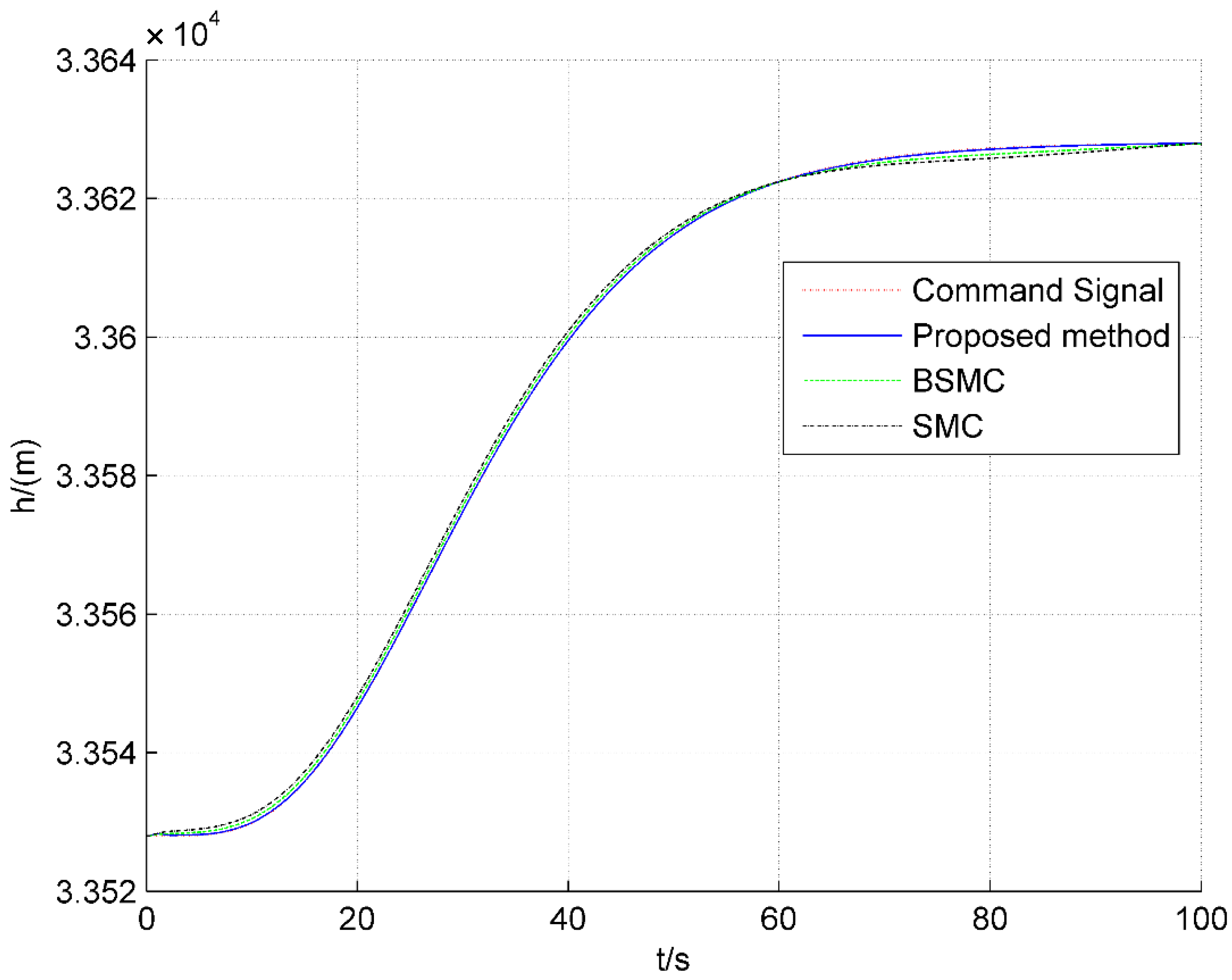
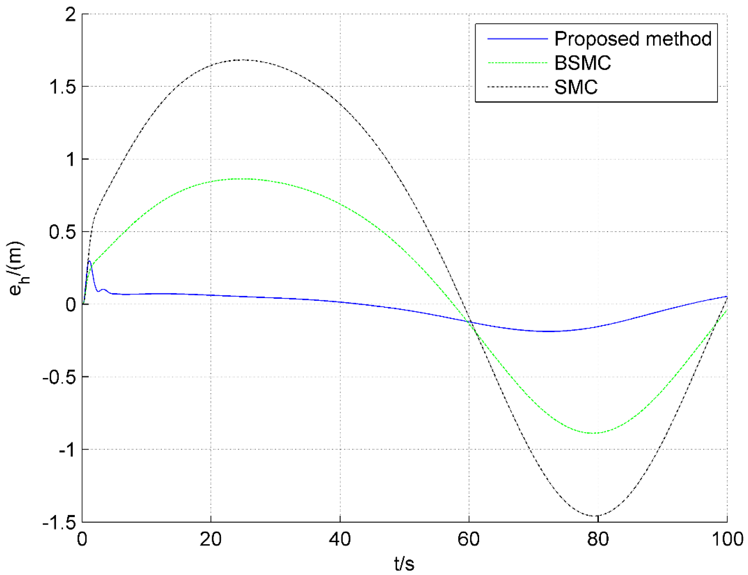
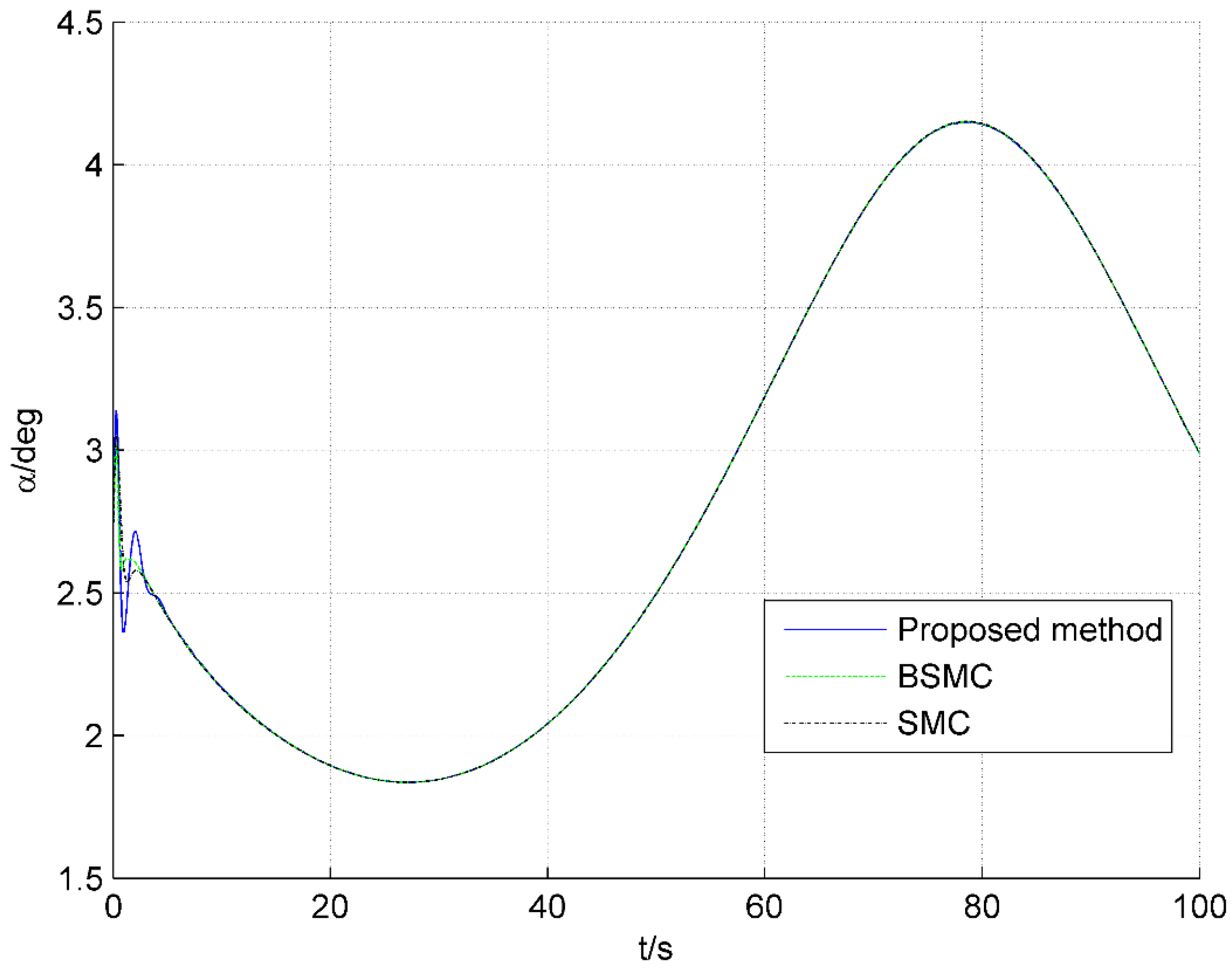
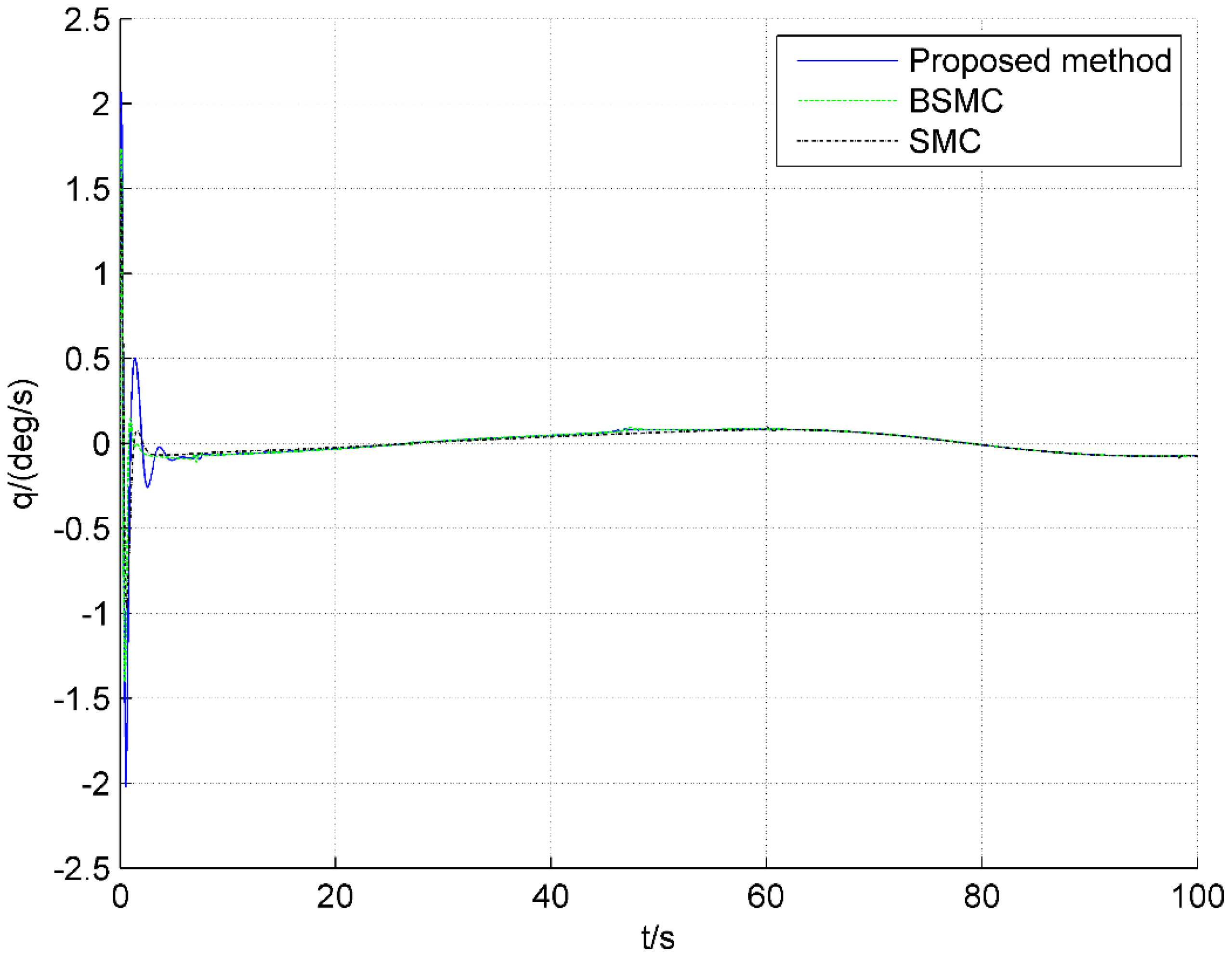
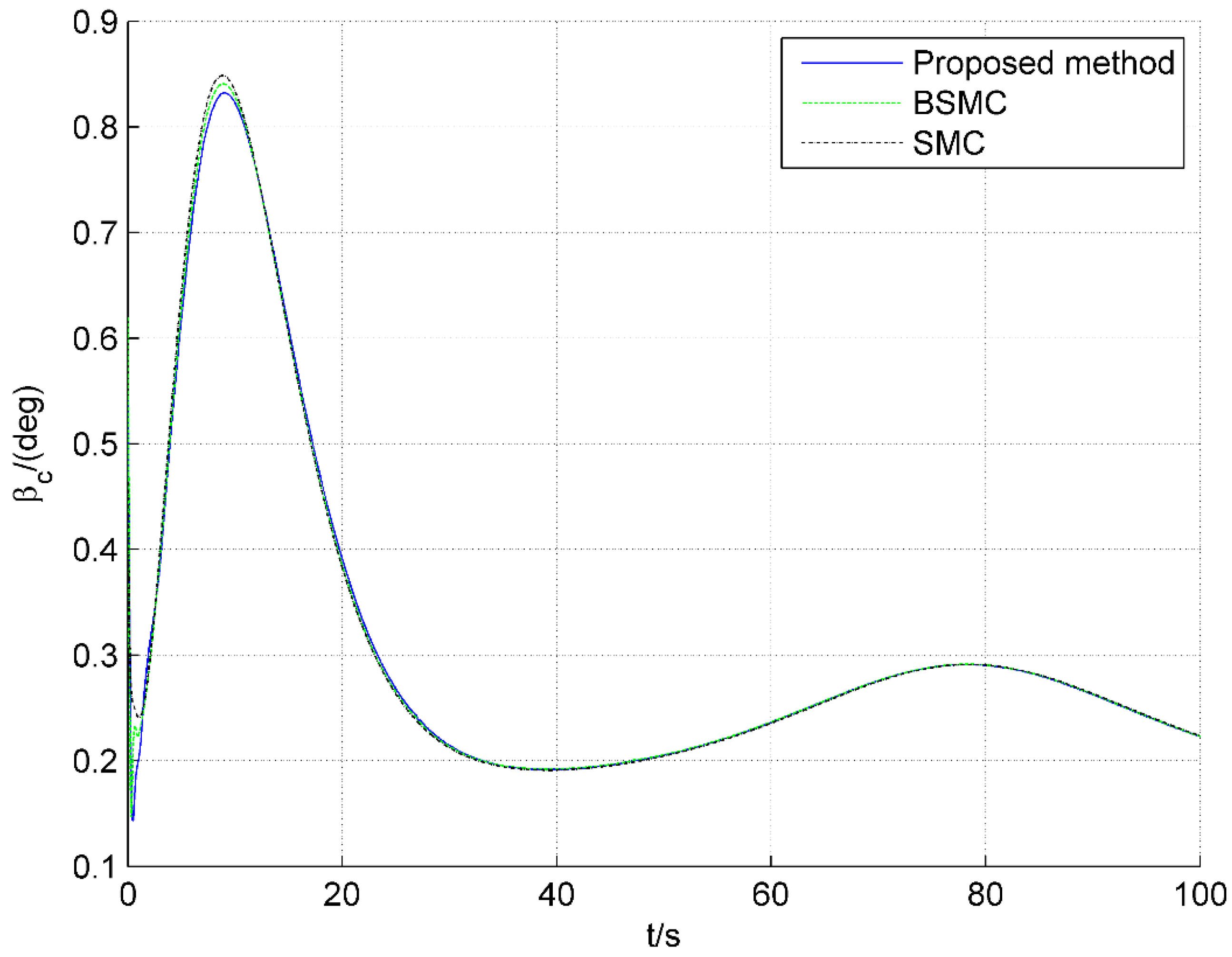
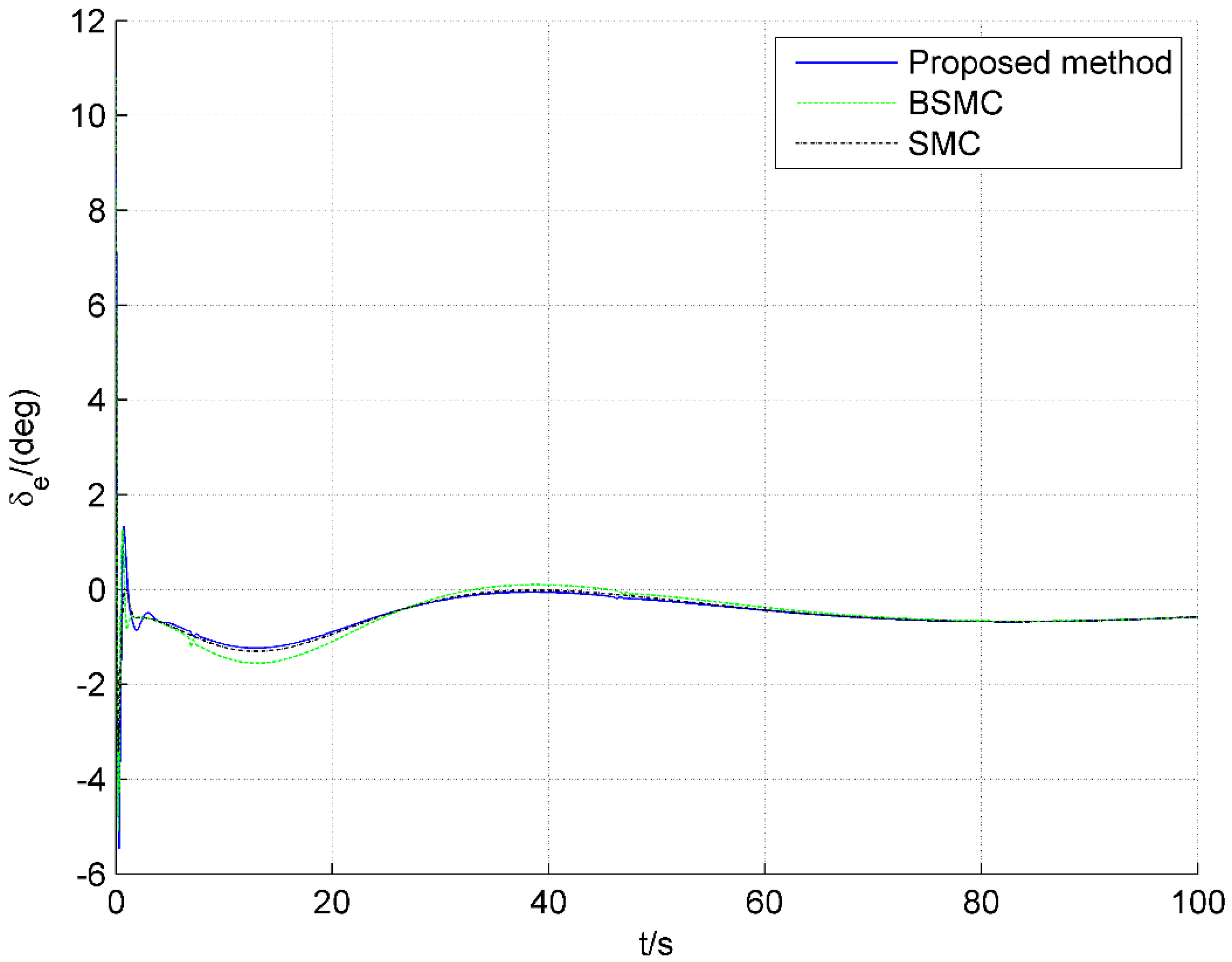
The proposed method in this paper shows better tracking performance than SMC and BSMC. Firstly, the tracking error of altitude and velocity under the proposed method in this paper is smaller than that for SMC or BSMC. Secondly, the responses of the flight path angle, attack angle, and pitch angle rate under the proposed method in this paper change smoothly and steadily. Thirdly, the control input change under the proposed method is smooth and within the acceptable range. Therefore, the proposed method achieves better flight performance than BSMC and SMC.

(2)

The method proposed in this paper can effectively attenuate the influence of uncertainties surrounding AHVs. Improved adaptive laws are adopted to compensate for the adverse influence of uncertainties on AHVs. The tracking errors (caused by uncertainties) under the proposed method are observed to be smaller than those of BSMC and SMC.

6. Conclusions

In this paper, a backstepping-based adaptive sliding mode controller is developed to ensure the performance of tracking control. First, a new double power reaching law for sliding mode is proposed, which guarantees the state of system converge to the equilibrium point within a fixed time. Secondly, to deal with uncertainties, a backstepping control for a high-order nonlinear system with uncertainties is established. Then, to enhance the robustness of the control system, the method of sliding mode control is incorporated into the backstepping design. Finally, to further reduce the effect of uncertainties on the AHV, adaptive laws of the control system are designed through Lyapunov. The control method designed in this paper can effectively compensate for the influence of mismatched uncertainties, with better robustness and good tracking performance.

References

1. Fan, Y.; Zhu, W.; Bai, G. A cost-effective tracking algorithm for hypersonic glide vehicle maneuver based on modified aerodynamic model. Appl. Sci. 2016, 6, 312. [Google Scholar] [CrossRef] [Green Version]
2. Zhang, J.; Sun, C.; Zhang, R.; Qian, C. Adaptive sliding mode control for re-entry attitude of near space hypersonic vehicle based on backstepping design. IEEE-CAA J. Automatic. 2015, 2, 94–101. [Google Scholar] [CrossRef]
3. Li, H.; Zhou, Y.; Wang, Y.; Du, S.; Xu, S. Optimal cruise characteristic analysis and parameter optimization method for air-breathing hypersonic vehicle. Appl. Sci. 2021, 11, 9565. [Google Scholar] [CrossRef]
4. Gao, H.; Chen, Z.; Sun, M.; Wang, Z.; Chen, Z. General periodic cruise guidance optimization for hypersonic vehicles. Appl. Sci. 2020, 10, 2898. [Google Scholar] [CrossRef] [Green Version]
5. Pu, Z.; Yuan, R.; Tan, X.; Yi, J. Active robust control of uncertainty and flexibility suppression for air-breathing hypersonic vehicles. Aerosp. Sci. Technol. 2015, 42, 429–441. [Google Scholar] [CrossRef]
6. Parker, J.T.; Serrani, A.; Yurkovich, S.; Bolender, M.A.; Doman, D.B. Control-oriented modeling of an air-breathing hypersonic vehicle. J. Guid. Control Dyn. 2007, 30, 856–869. [Google Scholar] [CrossRef]
7. Jiao, X.; Fidan, B.; Jiang, J.; Kamel, M. Type-2 fuzzy adaptive sliding mode control of hypersonic flight. Proc. Inst. Mech. Eng. Part G J. Aerosp. Eng. 2019, 233, 2731–2744. [Google Scholar] [CrossRef]
8. Zong, Q.; Ji, Y.; Zeng, F.; Liu, H. Output feedback backstepping control for a generic hypersonic vehicle via small-gain theorem. Aerosp. Sci. Technol. 2012, 23, 409–417. [Google Scholar] [CrossRef]
9. Su, X.; Jia, Y. Self-scheduled robust decoupling control with H∞ performance of hypersonic vehicles. Syst. Control Lett. 2014, 70, 38–48. [Google Scholar] [CrossRef]
10. Wu, H.; Feng, S.; Liu, Z.; Guo, L. Disturbance observer based robust mixed H2/H∞ fuzzy tracking control for hypersonic vehicles. Fuzzy Sets Syst. 2017, 306, 118–136. [Google Scholar] [CrossRef]
11. Shen, Q.; Jiang, B.; Cocquempot, V. Fault-tolerant control for T-S fuzzy systems with application to near-space hypersonic vehicle with actuator faults. IEEE Trans. Fuzzy Syst. 2012, 20, 652–665. [Google Scholar] [CrossRef]
12. Wang, Y.; Yang, X.; Yan, H. Reliable fuzzy tracking control of near-space hypersonic vehicle using aperiodic measurement information. IEEE Trans. Ind. Electron. 2019, 66, 9439–9447. [Google Scholar] [CrossRef]
13. Hu, X.; Wu, L.; Hu, C.; Wang, Z.; Gao, H. Dynamic output feedback control of a flexible air-breathing hypersonic vehicle via T-S fuzzy approach. Int. J. Syst. Sci. 2014, 45, 1740–1756. [Google Scholar] [CrossRef]
14. Xu, B.; Wang, D.; Zhang, Y.; Shi, Z. DOB-based neural control of flexible hypersonic flight vehicle considering wind effects. IEEE Trans. Ind. Electron. 2017, 64, 8676–8685. [Google Scholar] [CrossRef]
15. Xu, B.; Zhang, Q.; Pan, Y. Neural network based dynamic surface control of hypersonic flight dynamics using small-gain theorem. Neurocomputing 2016, 173, 690–699. [Google Scholar] [CrossRef]
16. Bu, X.; Wu, X.; Huang, J.; Ma, Z.; Zhang, R. Minimal-learning-parameter based simplified adaptive neural back-stepping control of flexible air-breathing hypersonic vehicles without virtual controllers. Neurocomputing 2016, 175, 816–825. [Google Scholar] [CrossRef]
17. Basin, M.V.; Yu, P.; Shtessel, Y.B. Hypersonic missile adaptive sliding mode control using finite- and fixed-time observers. IEEE Trans. Ind. Electron. 2018, 65, 930–941. [Google Scholar] [CrossRef]
18. Wang, J.; Wu, Y.; Dong, X. Recursive terminal sliding mode control for hypersonic flight vehicle with sliding mode disturbance observer. Nonlinear Dyn. 2015, 81, 1489–1510. [Google Scholar] [CrossRef]
19. Sun, H.; Li, S.; Sun, C. Finite time integral sliding mode control of hypersonic vehicles. Nonlinear Dyn. 2013, 73, 229–244. [Google Scholar] [CrossRef]
20. Guo, Z.; Chang, J.; Guo, J.; Zhou, J. Adaptive twisting sliding mode algorithm for hypersonic reentry vehicle attitude control based on finite-time observer. ISA Trans. 2018, 77, 20–29. [Google Scholar] [CrossRef]
21. Wu, G.; Meng, X. Nonlinear disturbance observer based robust backstepping control for a flexible air-breathing hypersonic vehicle. Aerosp. Sci. Technol. 2016, 54, 174–182. [Google Scholar] [CrossRef]
22. Ye, L.; Zong, Q.; Tian, B.; Zhang, X.; Wang, F. Control-oriented modeling and adaptive backstepping control for a nonminimum phase hypersonic vehicle. ISA Trans. 2017, 70, 161–172. [Google Scholar] [CrossRef] [PubMed]
23. Bu, X.; Wu, X.; Zhang, R.; Ma, Z.; Huang, J. Tracking differentiator design for the robust backstepping control of a flexible air-breathing hypersonic vehicle. J. Franklin Inst. 2015, 352, 1739–1765. [Google Scholar] [CrossRef]
24. Zong, Q.; Wang, F.; Tian, B.; Wang, J. Robust adaptive approximate backstepping control design for a flexible air-breathing hypersonic vehicle. J. Aerosp. Eng. 2015, 28, 04014107. [Google Scholar] [CrossRef]
25. An, H.; Xia, H.; Wang, C. Barrier lyapunov function-based adaptive control for hypersonic flight vehicles. Nonlinear Dyn. 2017, 88, 1833–1853. [Google Scholar] [CrossRef]
26. Hu, Q.; Wang, C.; Li, Y.; Huang, J. Adaptive control for hypersonic vehicles with time-varying faults. IEEE Trans. Aerosp. Electron. Syst. 2018, 54, 1442–1455. [Google Scholar] [CrossRef]
27. Liu, J.; An, H.; Gao, Y.; Wang, C.; Wu, L. Adaptive control of hypersonic flight vehicles with limited angle-of-attack. IEEE-ASME Trans. Mechatron. 2018, 23, 883–894. [Google Scholar] [CrossRef]
28. Fiorentini, L.; Serrani, A.; Bolender, M.A.; Doman, D.B. Nonlinear robust adaptive control of flexible air-breathing hypersonic vehicles. J. Guid. Control Dyn. 2009, 32, 402–417. [Google Scholar] [CrossRef]
29. Zhang, Y.; Li, R.; Xue, T.; Lei, Z. Exponential sliding mode tracking control via back-stepping approach for a hypersonic vehicle with mismatched uncertainty. J. Franklin Inst. 2016, 353, 2319–2343. [Google Scholar] [CrossRef]
30. Zong, Q.; Wang, F.; Su, R.; Shao, S. Robust adaptive backstepping tracking control for a flexible air-breathing hypersonic vehicle subject to input constraint. Proc. Inst. Mech. Eng. Part G J. Aerosp. Eng. 2015, 229, 10–25. [Google Scholar] [CrossRef]
31. Wang, S.; Jiang, J.; Yu, C. Adaptive backstepping sliding mode control of air-breathing hypersonic vehicles. Int. J. Aerosp. Eng. 2020, 2020, 8891051. [Google Scholar] [CrossRef]
32. Ma, G.; Chen, C.; Lyu, Y.; Guo, Y. Adaptive backstepping-based neural network control for hypersonic reentry vehicle with input constraints. IEEE Access 2018, 6, 1954–1966. [Google Scholar] [CrossRef]
33. Qi, R.; Huang, Y.; Jiang, B.; Tao, G. Adaptive backstepping control for a hypersonic vehicle with uncertain parameters and actuator faults. Proc. Inst. Mech. Eng. Part I J. Syst. Control. Eng. 2013, 227, 51–61. [Google Scholar] [CrossRef]
34. Hu, Q.; Meng, Y. Adaptive backstepping control for air-breathing hypersonic vehicle with actuator dynamics. Aerosp. Sci. Technol. 2017, 67, 412–421. [Google Scholar] [CrossRef]
35. Zong, Q.; Wang, J.; Tian, B.; Tao, Y. Quasi-continuous high-order sliding mode controller and observer design for flexible hypersonic vehicle. Aerosp. Sci. Technol. 2013, 27, 127–137. [Google Scholar] [CrossRef]
36. Mu, C.; Zong, Q.; Tian, B.; Xu, W. Continuous sliding mode controller with disturbance observer for hypersonic vehicles. IEEE-CAA J. Autom. 2015, 2, 45–55. [Google Scholar]
37. Zong, Q.; Dong, Q.; Wang, F.; Tian, B. Super twisting sliding mode control for a flexible air-breathing hypersonic vehicle based on disturbance observer. Sci. China Inf. Sci. 2015, 58, 1–15. [Google Scholar] [CrossRef] [Green Version]
38. Fallaha, C.J.; Saad, M.; Kanaan, H.Y.; Al-Haddad, K. Sliding-Mode robot control with exponential reaching law. IEEE Trans. Ind. Electron. 2011, 58, 600–610. [Google Scholar] [CrossRef]
39. Ke, D.; Wang, F.; He, L.; Li, Z. Predictive current control for PMSM systems using extended sliding mode observer with Hurwitz-based power reaching law. IEEE Trans. Power Electron. 2021, 36, 7223–7232. [Google Scholar] [CrossRef]
40. Xu, S.S.; Chen, C.; Wu, Z. Study of Nonsingular Fast Terminal Sliding-Mode Fault-Tolerant Control. IEEE Trans. Ind. Electron. 2015, 62, 3906–3913. [Google Scholar] [CrossRef]
41. Tao, M.; Chen, Q.; He, X.; Sun, M. Adaptive fixed-time fault-tolerant control for rigid spacecraft using a double power reaching law. Int. J. Robust Nonlinear Control 2019, 29, 4022–4040. [Google Scholar] [CrossRef]
42. Hu, X.; Wu, L.; Hu, C.; Gao, H. Adaptive sliding mode tracking control for a flexible air-breathing hypersonic vehicle. J. Franklin Inst. 2012, 349, 559–577. [Google Scholar] [CrossRef]
43. Wu, Y.; Zuo, J.; Sun, L. Adaptive terminal sliding mode control for hypersonic flight vehicles with strictly lower convex function based nonlinear disturbance observer. ISA Trans. 2017, 71, 215–226. [Google Scholar] [CrossRef] [PubMed]
44. Sagliano, M.; Mooij, E.; Theil, S. Adaptive disturbance-based high-order sliding-mode control for hypersonic-entry vehicles. J. Guid. Control Dyn. 2017, 40, 521–536. [Google Scholar] [CrossRef] [Green Version]
45. Xu, H.; Mirmirani, M.D.; Ioannou, P.A. Adaptive sliding mode control design for a hypersonic flight vehicle. J. Guid. Control Dyn. 2004, 27, 829–838. [Google Scholar] [CrossRef]
46. Xu, B.; Qi, R.; Jiang, B. Adaptive fault-tolerant control for HSV with unknown control direction. IEEE Trans. Aerosp. Electron. Syst. 2019, 55, 2743–2758. [Google Scholar] [CrossRef]
47. Yang, J.; Li, S.; Yu, X. Sliding-mode control for systems with mismatched uncertainties via a disturbance observer. IEEE Trans. Ind. Electron. 2013, 60, 160–169. [Google Scholar] [CrossRef]
Figure 1. Velocity tracking under reaching laws.
Applsci 12 06341 g001
Figure 2. Condition of s1 under reaching laws.
Applsci 12 06341 g002
Figure 3. Controller output, β c , under reaching laws.
Applsci 12 06341 g003
Figure 4. Responses of velocity tracking.
Applsci 12 06341 g004
Figure 5. Tracking errors of velocity.
Applsci 12 06341 g005
Figure 6. Responses of altitude tracking.
Applsci 12 06341 g006
Figure 7. Tracking errors of altitude.
Applsci 12 06341 g007
Figure 8. Responses of attack angle.
Applsci 12 06341 g008
Figure 9. Responses of pitch angle rate.
Applsci 12 06341 g009
Figure 10. Responses of throttle setting.
Applsci 12 06341 g010
Figure 11. Responses of elevator deflection.
Applsci 12 06341 g011