Semi-Analytical Planetary Landing Guidance with Constraint Equations Using Model Predictive Control

Abstract

With the deepening of planetary exploration, rapid decision making and descent trajectory planning capabilities are needed to cope with uncertain environmental disturbances and possible faults during planetary landings. In this article, a novel decoupling method is adopted, and the analytical three-dimensional constraint equations are derived and solved, ensuring real-time guidance computation. The three-dimensional motion modes and thrust profiles are analyzed and determined based on Pontryagin’s minimum principle, and a supporting semi-analytical reachability judgment method is presented, which can also be used to determine controllability. The algorithm is embedded in the model predictive control (MPC) framework, and several techniques are adopted to enhance stability and robustness, including thrust averaging, thrust correction after ignition, thrust reservation, and open-loop terminal guidance. Numerical simulations demonstrate that the proposed algorithm can guarantee real-time trajectory generation and meanwhile maintain considerable optimality. In addition, the MPC simulation shows that the algorithm can maintain a good accuracy under external disturbances.

1. Introduction

With the success of a series of planetary exploration missions, researchers’ understanding of the planetary characteristics and planetary landing is more and more in depth [1,2], and more appropriate potential landing target points will be found [3]. Due to the uncertain planetary environmental factors and possible faults of the lander [4,5], the actual trajectory may deviate from the preset trajectory or even make the origin landing point unreachable. At this time, how to rapidly determine the reachable landing points from potential landing target points and plan the trajectory online brings new challenges for powered descent guidance algorithms. Therefore, rapid decision making and real-time trajectory planning methods will be the key to mission success.

Powered decent guidance is essentially a trajectory optimization problem, which can be traditionally solved by indirect methods or direct methods. Based on the optimal control theory, the indirect method converts the optimal control problem into a two-point boundary value problem by introducing the costates [6,7]. However, it is difficult to guarantee the convergence due to the difficulty in estimating the initial values of the costates [8]. In contrast, the direct method is more widely used in powered descent guidance [9], because it can handle complex dynamic models with multiple constraints and has a slightly wider convergence domain. Acikmese et al. proposed a lossless convex programming approach and successfully applied it to powered descent guidance for Mars landing [10,11,12,13]. However, for the problem of free final time, the lossless convex programming approach cannot achieve real-time planning due to the inaccuracy of final time prediction [14]. Subsequent studies include sequential convex optimization [15,16,17,18] and successive convex optimization [19,20,21,22]. These convex optimization methods can deal with more complex constraints and dynamics (e.g., the problem with free final time and flight angle constraints) through linearization and the introduction of trust region, virtual control, and virtual buffer. The cost is the occupation of more computational resources and the decrease in computational efficiency caused by iteration. The pseudospectral convex optimization method [23,24,25] improves the accuracy by adopting the pseudospectral discretization, but the efficiency is not greatly improved.

The research on real-time powered descent guidance control actually began in the 1960s [26], and the very famous application is the successful lunar landing of Apollo 11. Due to the limitation of the computing ability, Apollo 11 adopted the polynomial guidance method which derived an analytical expression for the acceleration command with the remaining flight time [27]. The subsequent studies further investigated the constrained optimal thrust acceleration vector profile by adopting different decoupling methods and derived elegant analytical expressions [28,29,30,31,32,33]. The commonness of these analytical methods is to analyze the thrust acceleration rather than the thrust. As a result, these methods cannot rapidly and accurately determine the reachability of the landing point in the current state. With the development of artificial intelligence, some researchers apply learning-based methods to powered descent guidance [34,35]. These methods can achieve high accuracy and efficiency in theory with a large and accurate training set, but the performance of these methods is not stable enough in the face of unexpected situations [14].

Model predictive control (MPC) is a popular advanced method to control dynamical systems subject to uncertain disturbances and possible faults [36,37,38]. In Ref. [36], a robust nonlinear multi-variable predictive control under constraints was proposed and solved using a linear matrix inequalities (LMIs) formation. Bououden et al. proposed a robust MPC algorithm for active suspension systems with time-varying delays and input constraints [37]. In Ref. [38], the sensor and actuator faults were considered and a robust fault-tolerant model predictive control approach was proposed. By minimizing the upper bound of the objective function, the MPC state feedback law is obtained in terms of linear matrix inequalities (LMIs). Simulation results have illustrated the effectiveness of these methods. Different from the above methods, we focus more on the optimization algorithm than the MPC framework. In order to confirm the robust stability of the closed-loop system, the efficiency and reliability of the optimization algorithm should be guaranteed first.

This article proposes a rapid semi-analytical powered descent guidance algorithm for planetary landing. By using this algorithm, the following two aims are achieved: (1) real-time guidance computation and (2) rapid reachability/controllability determination. To achieve real-time guidance computation, a decoupling method is adopted and the fuel-optimal control mode is derived. Six explicit constraint equations are obtained and the solutions of which are in closed form, so that the real-time guidance computation is guaranteed. In order to make full use of the real-time advantages of the analytical method, and improve the performance of the proposed method in the face of practical complex constraints, the model predictive control framework is chosen. Several techniques are adopted to guarantee the recursive feasibility.

The article is organized as follows. In Section 2, the planetary landing guidance is first transformed into an optimal control problem, and the optimal solution for the one-dimensional problem is derived. Then, a dynamic decoupling method is introduced, and the decoupled three-dimensional fuel-optimal control modes are derived through Pontryagin’s maximum principle. In Section 3, the motion modes in three directions are analyzed in detail, and the reachability determination method is presented. In Section 4, we apply our semi-analytical algorithm to model the predictive control framework and adopt several techniques to enhance the robustness. The simulation results are presented in Section 5, and conclusions are summarized in Section 6.

2. Problem Description and Decoupled Trajectory Planning

In this section, we transform the planetary landing guidance into an optimal control problem and introduce a three-dimensional decoupling method. In Section 2.1, we review the one-dimensional problem, and the optimal control mode which consists of either full thrust or a period of zero thrust followed by full thrust is obtained [26]. In Section 2.2, we apply the one-dimensional optimal control mode in the three-dimensional problem and assume that the proportion of the thrust for horizontal control is fixed after ignition. Based on Pontryagin’s maximum principle, we derive that the direction of horizontal thrust changes at most once after ignition. This decoupling method significantly reduces the difficulty of the three-dimensional analytical derivation, despite sacrificing some optimality and control smoothness.

2.1. One-Dimensional Analytical Derivation

Assume that the one-dimension motion of the lander is vertical and subject to the following assumptions [26]: (a) the only forces acting on the lander are gravity and thrust, i.e., aerodynamic effects are ignored, (b) the thrust direction can only be vertical upward, (c) the gravitational acceleration is constant, (d) the propulsion system is capable of mass flow rates between zero and a fixed upper limit, (e) the landing point is set to be the origin, and the vertical upward is positive. Under these assumptions, the dynamic equations are expressed as:

$$\dot{r}\left(t\right)=v\left(t\right)$$

(1)

$$\dot{v}\left(t\right)={\displaystyle \frac{T_{\max }}{m\left(t\right)}}u\left(t\right)-g$$

(2)

$$\dot{m}\left(t\right)=-{\displaystyle \frac{T_{\max }}{I_{\mathrm{sp}}{g}_0}}u\left(t\right)$$

(3)

where $r\left(t\right)$, $v\left(t\right)$, and $m\left(t\right)$ are the lander’s position, velocity, and mass, respectively; $T_{\max }$ is the max amplitude of thrust; g is the absolute value of gravity acceleration; $u\left(t\right)(0\le u(t)\le 1)$ is the control, $I_{\mathrm{sp}}$ is the specific impulse, and $g_0$ is the standard gravity, equal to 9.807 $\mathrm{m}/{\mathrm{s}}^2$.

By eliminating $u\left(t\right)$, we obtain

$$\dot{v}\left(t\right)=-I_{\mathrm{sp}}{g}_0{\displaystyle \frac{\dot{m}\left(t\right)}{m}}-g$$

(4)

By denoting the final time as $t_{\mathrm{f}}$, and integrating Equation (4) from 0 to $t_{\mathrm{f}}$, we obtain

$$m_{\mathrm{f}}=m_0\exp \left({\displaystyle \frac{v_0-g{t}_{\mathrm{f}}}{I_{\mathrm{sp}}{g}_0}}\right)$$

(5)

where $m_0$, $v_0$, and $m_{\mathrm{f}}$ are the initial mass, initial velocity, and final mass, respectively. It is shown that the final mass is a strictly monotonic decreasing function of the final time $t_{\mathrm{f}}$. Therefore, minimizing the final time $t_{\mathrm{f}}$ is equivalent to minimizing the fuel consumption.

The time-minimum problem is now considered. The performance index is chosen as

$$J={\int }_{t_0}^{t_{\mathrm{f}}}1dt$$

(6)

The Hamiltonian for this optimal problem is

$$H(\mathbf{s},u,\mathbf{\lambda })=1+{\lambda }_{\mathrm{r}}v+{\lambda }_{\mathrm{v}}\left({\displaystyle \frac{T_{\max }}{m}}u-g\right)-{\lambda }_{\mathrm{m}}{\displaystyle \frac{T_{\max }}{I_{\mathrm{sp}}{g}_0}}u$$

(7)

where $\mathbf{s}={[r,v,m]}^T$ represents the state variables, and $\mathbf{\lambda }={[{\lambda }_{\mathrm{r}},{\lambda }_{\mathrm{v}},{\lambda }_{\mathrm{m}}]}^T$ are costate variables, which satisfy the Euler–Lagrange condition:

$$\dot{\mathbf{\lambda }}=-{\displaystyle \frac{\partial H({\mathbf{s}}^{*},u^{*},\mathbf{\lambda })}{\partial {\mathbf{s}}^{*}}}$$

(8)

Therefore,

$${\dot{\lambda }}_{\mathrm{r}}=0,{\dot{\lambda }}_{\mathrm{v}}=-{\lambda }_{\mathrm{r}},{\dot{\lambda }}_{\mathrm{m}}={\lambda }_{\mathrm{v}}{\displaystyle \frac{T_{\max }}{m^2}}u$$

(9)

According to Pontryagin’s minimum principle, the form of the optimal control $u^{*}$ is obtained:

$$u^{*}\left(t\right)\left\{\begin{array}{c}=0,\xi >0\hfill \\ =1,\xi <0\hfill \\ \in [0,1],\xi =0\hfill \end{array}\right.$$

(10)

where $\xi ={\lambda }_{\mathrm{v}}{T}_{\max }/m-{\lambda }_{\mathrm{m}}{T}_{\max }/I_{\mathrm{sp}}/g_0$. According to Equation (10), $u^{*}$ holds singular only if $\xi =0$. In Ref. [26], Meditch rigorously proved that (1) the singularity condition could not hold on any finite closed interval in $[0,t_{\mathrm{f}}]$ and (2) there was at most one switching in $[0,t_{\mathrm{f}}]$. In other words, the time optimal control of this one-dimension problem has only two modes: $u\left(t\right)=1,t\in [0,t_{\mathrm{f}}]$ or $u\left(t\right)=0,t\in [0,t_1];u\left(t\right)=1,t\in (t_1,t_{\mathrm{f}}]$, where $t_1$ is the ignition time.

By setting the final velocity and position, which are obtained by integrating the dynamic equations from 0 through $t_1$ to $t_{\mathrm{f}}$, equal to 0, we obtain two nonlinear constraint equations, with the ignition time $t_1$ and the final time $t_{\mathrm{f}}$ as unknown variables, as follows:

$$\begin{array}{cccc}\hfill & \hfill & \hfill v\left(t_{\mathrm{f}}\right)& =v_0-g{t}_{\mathrm{f}}+{\displaystyle \frac{T_{\max }}{\eta }}ln\left({\displaystyle \frac{m_0}{\eta }}\right)-{\displaystyle \frac{T_{\max }}{\eta }}ln\left({\displaystyle \frac{m_0}{\eta }}-(t_{\mathrm{f}}-t_1)\right)\hfill \\ \hfill & \hfill & \hfill & =0\hfill \end{array}$$

(11)

$$\begin{array}{cccc}\hfill & \hfill & \hfill r\left(t_{\mathrm{f}}\right)& =r_0+v_0{t}_{\mathrm{f}}-{\displaystyle \frac{1}{2}}g{t_{\mathrm{f}}}^2+{\displaystyle \frac{T_{\max }}{\eta }}ln\left({\displaystyle \frac{m_0}{\eta }}\right)(t_{\mathrm{f}}-t_1)+{\displaystyle \frac{T_{\max }}{\eta }}(t_{\mathrm{f}}-t_1)\hfill \\ \hfill & \hfill & \hfill & +{\displaystyle \frac{T_{\max }}{\eta }}\left. [\left({\displaystyle \frac{m_0}{\eta }}-(t_{\mathrm{f}}-t_1)\right)ln\left({\displaystyle \frac{m_0}{\eta }}-(t_{\mathrm{f}}-t_1)\right)-{\displaystyle \frac{m_0}{\eta }}ln\left({\displaystyle \frac{m_0}{\eta }}\right)\right]\hfill \\ \hfill & \hfill & \hfill & =0\hfill \end{array}$$

(12)

where $r_0$ is the initial position, and $\eta =T_{\max }/I_{\mathrm{sp}}/g_0$ is the absolute value of mass flow.

2.2. Three-Dimensional Extension

Setting the current position of the lander as the starting point and the target landing point as the origin, we construct the X-Z plane with the vertical direction. The positive direction of the Z-axis is vertical upward. The X-axis’s positive direction is from the landing point to the horizontal projection of the starting point. The Y-axis forms a right-handed coordinate system with X and Z axes, as shown in Figure 1. In this coordinate system, $x_0$ is always greater than or equal to 0, and $y_0$ is always equal to 0.

To allow analytic treatment of a portion of the dynamics, one decoupling assumption is introduced: the lander first experiences a period of unpowered landing with an initial velocity; then, the engines switch on at $t_1$, and the lander lands on the ground at $t_{\mathrm{f}}$. After the ignition time $t_1$, ${\mu }_{\mathrm{x}}{T}_{\max }$ is used to adjust the position and velocity in the X direction, ${\mu }_{\mathrm{y}}{T}_{\max }$ is used in the Y direction, and $\sqrt{1-{\mu }_{\mathrm{x}}^2-{\mu }_{\mathrm{y}}^2}{T}_{\max }$, denoted as ${\mu }_{\mathrm{z}}{T}_{\max }$, is used for vertical deceleration ($0\le {\mu }_{\mathrm{x},\mathrm{y},\mathrm{z}}\le 1$). To further reduce the complexity caused by the unfixed mass flow, we assume that the adjustments in three directions begin simultaneously at $t_1$ and stop simultaneously at the final time $t_{\mathrm{f}}$. Then, the mass flow rate of the lander after ignition is a constant parameter, and its value is equal to $-\eta$.

Under this control mode, the decoupled dynamic equations after $t_1$ are expressed as:

$${[\dot{x}\left(t\right),\dot{y}\left(t\right),\dot{z}\left(t\right)]}^T={[v_{\mathrm{x}}\left(t\right),v_{\mathrm{y}}\left(t\right),v_{\mathrm{z}}\left(t\right)]}^T$$

(13)

$${[{\dot{v}}_{\mathrm{x}}\left(t\right),{\dot{v}}_{\mathrm{y}}\left(t\right),{\dot{v}}_{\mathrm{z}}\left(t\right)]}^T={\left. [{\displaystyle \frac{{\mu }_{\mathrm{x}}{T}_{\max }}{m\left(t\right)}}{\alpha }_{\mathrm{x}}\left(t\right),{\displaystyle \frac{{\mu }_{\mathrm{y}}{T}_{\max }}{m\left(t\right)}}{\alpha }_{\mathrm{y}}\left(t\right),{\displaystyle \frac{{\mu }_{\mathrm{z}}{T}_{\max }}{m\left(t\right)}}-g\right]}^T$$

(14)

$$\dot{m}\left(t\right)=-\eta$$

(15)

where ${\alpha }_{\mathrm{x}}\left(t\right),{\alpha }_{\mathrm{y}}\left(t\right)\in \{-1,1\}$ represent the X- and Y- thrust directions, respectively.

Then, we will analyze the form of ${\alpha }_{\mathrm{x}}\left(t\right)$ and ${\alpha }_{\mathrm{y}}\left(t\right)$ through Pontryagin’s maximum principle.

The performance index is chosen as

$$J={\int }_{t_1}^{t_{\mathrm{f}}}\eta dt$$

(16)

The Hamiltonian for this optimal control problem is

$$\begin{array}{cc}\hfill H=& \eta -{\lambda }_{\mathrm{m}}\eta +[{\lambda }_{\mathrm{x}},{\lambda }_{\mathrm{y}},{\lambda }_{\mathrm{z}}]·{[v_{\mathrm{x}}\left(t\right),v_{\mathrm{y}}\left(t\right),v_{\mathrm{z}}\left(t\right)]}^T\hfill \\ \hfill & +[{\lambda }_{\mathrm{vx}},{\lambda }_{\mathrm{vy}},{\lambda }_{\mathrm{vz}}]·{\left. [{\displaystyle \frac{{\mu }_{\mathrm{x}}{T}_{\max }}{m\left(t\right)}}{\alpha }_{\mathrm{x}}\left(t\right),{\displaystyle \frac{{\mu }_{\mathrm{y}}{T}_{\max }}{m\left(t\right)}}{\alpha }_{\mathrm{y}}\left(t\right),{\displaystyle \frac{{\mu }_{\mathrm{z}}{T}_{\max }}{m\left(t\right)}}-g\right]}^T\hfill \end{array}$$

(17)

where ${\lambda }_{\mathrm{m}}$, ${\mathbf{\lambda }}_{\mathrm{r}}={[{\lambda }_{\mathrm{x}},{\lambda }_{\mathrm{y}},{\lambda }_{\mathrm{z}}]}^T$, and ${\mathbf{\lambda }}_{\mathrm{v}}={[{\lambda }_{\mathrm{vx}},{\lambda }_{\mathrm{vy}},{\lambda }_{\mathrm{vz}}]}^T$ are costate variables, which satisfy the Euler–Lagrange condition:

$${\dot{\lambda }}_{\mathrm{m}}=-{\displaystyle \frac{\partial H}{\partial m}}$$

(18)

$${[{\dot{\lambda }}_{\mathrm{x}},{\dot{\lambda }}_{\mathrm{y}},{\dot{\lambda }}_{\mathrm{z}}]}^T={\left. [-{\displaystyle \frac{\partial H}{\partial x}},-{\displaystyle \frac{\partial H}{\partial y}},-{\displaystyle \frac{\partial H}{\partial z}}\right]}^T={[0,0,0]}^T$$

(19)

$${[{\dot{\lambda }}_{\mathrm{vx}},{\dot{\lambda }}_{\mathrm{vy}},{\dot{\lambda }}_{\mathrm{vz}}]}^T={\left. [-{\displaystyle \frac{\partial H}{\partial v_{\mathrm{x}}}},-{\displaystyle \frac{\partial H}{\partial v_{\mathrm{y}}}},-{\displaystyle \frac{\partial H}{\partial v_{\mathrm{z}}}}\right]}^T={[-{\lambda }_{\mathrm{x}},-{\lambda }_{\mathrm{y}},-{\lambda }_{\mathrm{z}}]}^T$$

(20)

The solutions of Equations (19) and (20) can be expressed as

$${[{\lambda }_{\mathrm{x}},{\lambda }_{\mathrm{y}},{\lambda }_{\mathrm{z}}]}^T={[C_1,C_2,C_3]}^T$$

(21)

$${[{\lambda }_{\mathrm{vx}},{\lambda }_{\mathrm{vy}},{\lambda }_{\mathrm{vz}}]}^T={[-C_{1}t+D_1,-C_{2}t+D_2,-C_{3}t+D_3]}^T$$

(22)

where $C_{1\sim 3}$ and $D_{1\sim 3}$ are constant.

According to the Pontryagin’s minimum principle, the optimal ${\alpha }_{\mathrm{x}}^{*}$ and ${\alpha }_{\mathrm{y}}^{*}$ are obtained

$${\alpha }_{\mathrm{x}\left(\mathrm{y}\right)}^{*}\left\{\begin{array}{c}=-1,{\lambda }_{\mathrm{vx}\left(\mathrm{vy}\right)}>0\hfill \\ =1,{\lambda }_{\mathrm{vx}\left(\mathrm{vy}\right)}<0\hfill \\ \in \{-1,1\},{\lambda }_{\mathrm{vx}\left(\mathrm{vy}\right)}=0\hfill \end{array}\right.$$

(23)

where ${\alpha }_{\mathrm{x}\left(\mathrm{y}\right)}^{*}$ are singular when ${\lambda }_{\mathrm{vx}\left(\mathrm{vy}\right)}=0$. According to Equation (22), ${\alpha }_{\mathrm{x}\left(\mathrm{y}\right)}^{*}$ hold singular only if $\{C_{1\left(2\right)},D_{1\left(2\right)}\}=\{0,0\}$. For these cases, the costate variables ${\lambda }_{\mathrm{x}}$, ${\lambda }_{\mathrm{y}}$, ${\lambda }_{\mathrm{vx}}$, and ${\lambda }_{\mathrm{vy}}$ equal zero for the whole flight. Neglecting these singular cases, there is at most one isolated singular point. This also means that the thrust direction in the X (or Y) direction switches at most once after $t_1$.

3. Motion Mode Analysis and Reachability Determination

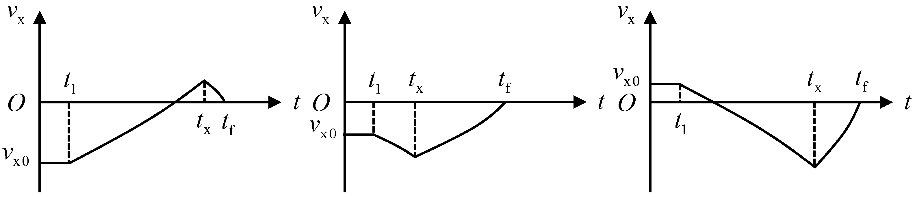
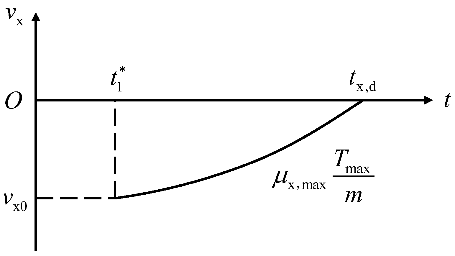
3.1. Motion Mode Analysis

We first analyze the motion mode in the Y direction. As mentioned in Section 2.2, ${\mu }_{\mathrm{y}}{T}_{\max }$ is used to adjust the position and velocity in the Y direction, and the thrust direction switches at most once. Because the target displacement in the Y direction is 0, the motion modes in the Y direction are divided into only two kinds: (a) when $v_{\mathrm{y}0}>0$, the thrust in the Y direction should be negative first and then positive; (b) when $v_{\mathrm{y}0}<0$, the thrust in the Y direction should be positive first and then negative. By denoting $t_{\mathrm{y}}$ as the moment when the thrust direction changes, the two kinds of motion modes in the Y direction are schematically shown in Figure 2.

Then, the motion mode in the X direction is analyzed. Based on the thrust direction change and the initial velocity $v_{\mathrm{x}0}$, the motion modes in the X direction are divided into three categories: (a) when $v_{\mathrm{x}0}<0$ and the absolute value of $v_{\mathrm{x}0}$ is relatively large, to meet terminal constraints, the thrust in the X direction should be positive first and then negative; (b) when $v_{\mathrm{x}0}<0$ and the absolute value of $v_{\mathrm{x}0}$ is relatively small, the thrust should be negative first and then positive; c) when $v_{\mathrm{x}0}\ge 0$, the thrust should be negative first and then positive. By denoting $t_{\mathrm{x}}$ as the moment when the thrust direction changes, the three motion modes in the X direction are schematically shown in Figure 3. Whether the value of $v_{\mathrm{x}0}$ is large or small will be discussed in detail in Section 3.2.

We introduce two variables, ${\gamma }_{\mathrm{y}}$ and ${\gamma }_{\mathrm{x}}$, to describe the motion modes in the Y and X directions, respectively. If the thrust in the Y direction is positive first and then negative, ${\gamma }_{\mathrm{y}}=1$; if the thrust is negative first and then positive, ${\gamma }_{\mathrm{y}}=-1$; if $v_{\mathrm{y}0}=0$, ${\gamma }_{\mathrm{y}}=0$. The value of ${\gamma }_{\mathrm{x}}$ is assigned in the same way. Taking the derivation in the X direction as an example, we will show the derivation process of explicit constraint equations in detail. The dynamic equation in the X direction is as follows:

$${\dot{v}}_{\mathrm{x}}\left(t\right)=\left\{\begin{array}{c}0,t\in [0,t_1]\hfill \\ {\gamma }_{\mathrm{x}}{\displaystyle \frac{{\mu }_{\mathrm{x}}{T}_{\max }}{m_0-\eta (t-t_1)}},t\in (t_1,t_{\mathrm{x}}]\hfill \\ -{\gamma }_{\mathrm{x}}{\displaystyle \frac{{\mu }_{\mathrm{x}}{T}_{\max }}{m_0-\eta (t-t_1)}},t\in (t_{\mathrm{x}},t_{\mathrm{f}}]\hfill \end{array}\right.$$

(24)

By integration, the explicit expression of $v_{\mathrm{x}}\left(t\right)$ is obtained as follows:

$$v_{\mathrm{x}}\left(t\right)=\left\{\begin{array}{c}{v}_{\mathrm{x}0},t\in [0,t_1]\hfill \\ {\gamma }_{\mathrm{x}}{\displaystyle \frac{{\mu }_{\mathrm{x}}{T}_{\max }}{\eta }}\left. [ln\left({\displaystyle \frac{m_0}{\eta }}\right)-ln\left({\displaystyle \frac{m_0}{\eta }}-(t-t_1)\right)\right]+v_{\mathrm{x}0},t\in (t_1,t_{\mathrm{x}}]\hfill \\ {\gamma }_{\mathrm{x}}{\displaystyle \frac{{\mu }_{\mathrm{x}}{T}_{\max }}{\eta }}\left. [ln\left({\displaystyle \frac{m_0}{\eta }}-(t-t_1)\right)-ln\left({\displaystyle \frac{m_0}{\eta }}-(t_{\mathrm{x}}-t_1)\right)\right]+v_{\mathrm{x}}\left(t_{\mathrm{x}}\right),t\in (t_{\mathrm{x}},t_{\mathrm{f}}]\hfill \end{array}\right.$$

(25)

Then, the terminal velocity and position constraints in the X direction can be expressed as:

$$\begin{array}{cccc}\hfill & \hfill & \hfill v_{\mathrm{x}}\left(t_{\mathrm{f}}\right)& ={\gamma }_{\mathrm{x}}{\displaystyle \frac{{\mu }_{\mathrm{x}}{T}_{\max }}{\eta }}\left. [ln\left({\displaystyle \frac{m_0}{\eta }}\right)+ln\left({\displaystyle \frac{m_0}{\eta }}-(t_{\mathrm{f}}-t_1)\right)-2ln\left({\displaystyle \frac{m_0}{\eta }}-(t_{\mathrm{x}}-t_1)\right)\right]+v_{\mathrm{x}0}\hfill \\ \hfill & \hfill & \hfill & =0\hfill \end{array}$$

(26)

$$\begin{array}{cccc}\hfill & \hfill & \hfill x\left(t_{\mathrm{f}}\right)& ={\int }_0^{t_1}{v}_{\mathrm{x}}\left(t\right)dt+{\int }_{t_1}^{t_{\mathrm{x}}}{v}_{\mathrm{x}}\left(t\right)dt+{\int }_{t_{\mathrm{x}}}^{t_{\mathrm{f}}}{v}_{\mathrm{x}}\left(t\right)dt\hfill \\ \hfill & \hfill & \hfill & =x_0+v_{\mathrm{x}0}{t}_{\mathrm{f}}+{\gamma }_{\mathrm{x}}{\displaystyle \frac{{\mu }_{\mathrm{x}}{T}_{\max }}{\eta }}ln\left({\displaystyle \frac{m_0}{\eta }}\right)(t_{\mathrm{f}}-t_1)+{\gamma }_{\mathrm{x}}{\displaystyle \frac{{\mu }_{\mathrm{x}}{T}_{\max }}{\eta }}(2t_{\mathrm{x}}-t_1-t_{\mathrm{f}})\hfill \\ \hfill & \hfill & \hfill & +{\gamma }_{\mathrm{x}}{\displaystyle \frac{2{\mu }_{\mathrm{x}}{T}_{\max }}{\eta }}\left({\displaystyle \frac{m_0}{\eta }}-(t_{\mathrm{x}}-t_1)\right)\left. [ln\left({\displaystyle \frac{m_0}{\eta }}-(t_{\mathrm{x}}-t_1)\right)-(t_{\mathrm{f}}-t_{\mathrm{x}})\right]\hfill \\ \hfill & \hfill & \hfill & -{\gamma }_{\mathrm{x}}{\displaystyle \frac{{\mu }_{\mathrm{x}}{T}_{\max }}{\eta }}\left. [\left({\displaystyle \frac{m_0}{\eta }}-(t_{\mathrm{f}}-t_1)\right)ln\left({\displaystyle \frac{m_0}{\eta }}-(t_{\mathrm{f}}-t_1)\right)+{\displaystyle \frac{m_0}{\eta }}ln\left({\displaystyle \frac{m_0}{\eta }}\right)\right]\hfill \\ \hfill & \hfill & \hfill & =0\hfill \end{array}$$

(27)

Similarly, the explicit constraint equations in the Y direction can also be obtained. Furthermore, the explicit constraint equations in the Z direction can be extended from one-dimensional constraint equations. Then, the complete constraint equations corresponding to the terminal velocity and position constraints in the Z, Y, and X directions, respectively, are expressed as follows:

$$\begin{array}{cccc}\hfill & \hfill & \hfill v_{\mathrm{z}}\left(t_{\mathrm{f}}\right)& =v_{\mathrm{z}0}-g{t}_{\mathrm{f}}+{\displaystyle \frac{{\mu }_{\mathrm{z}}{T}_{\max }}{\eta }}ln\left({\displaystyle \frac{m_0}{\eta }}\right)-{\displaystyle \frac{{\mu }_{\mathrm{z}}{T}_{\max }}{\eta }}ln\left({\displaystyle \frac{m_0}{\eta }}-(t_{\mathrm{f}}-t_1)\right)\hfill \\ \hfill & \hfill & \hfill & =0\hfill \end{array}$$

(28)

$$\begin{array}{cccc}\hfill & \hfill & \hfill z\left(t_{\mathrm{f}}\right)& =z_0+v_{\mathrm{z}0}{t}_{\mathrm{f}}-{\displaystyle \frac{1}{2}}g{t_{\mathrm{f}}}^2+{\displaystyle \frac{{\mu }_{\mathrm{z}}{T}_{\max }}{\eta }}ln\left({\displaystyle \frac{m_0}{\eta }}\right)(t_{\mathrm{f}}-t_1)+{\displaystyle \frac{{\mu }_{\mathrm{z}}{T}_{\max }}{\eta }}(t_{\mathrm{f}}-t_1)\hfill \\ \hfill & \hfill & \hfill & +{\displaystyle \frac{{\mu }_{\mathrm{z}}{T}_{\max }}{\eta }}\left. [\left({\displaystyle \frac{m_0}{\eta }}-(t_{\mathrm{f}}-t_1)\right)ln\left({\displaystyle \frac{m_0}{\eta }}-(t_{\mathrm{f}}-t_1)\right)-{\displaystyle \frac{m_0}{\eta }}ln\left({\displaystyle \frac{m_0}{\eta }}\right)\right]\hfill \\ \hfill & \hfill & \hfill & =0\hfill \end{array}$$

(29)

$$\begin{array}{cccc}\hfill & \hfill & \hfill v_{\mathrm{y}}\left(t_{\mathrm{f}}\right)& ={\gamma }_{\mathrm{y}}{\displaystyle \frac{{\mu }_{\mathrm{y}}{T}_{\max }}{\eta }}\left. [ln\left({\displaystyle \frac{m_0}{\eta }}\right)+ln\left({\displaystyle \frac{m_0}{\eta }}-(t_{\mathrm{f}}-t_1)\right)-2ln\left({\displaystyle \frac{m_0}{\eta }}-(t_{\mathrm{y}}-t_1)\right)\right]+v_{\mathrm{y}0}\hfill \\ \hfill & \hfill & \hfill & =0\hfill \end{array}$$

(30)

$$\begin{array}{cccc}\hfill & \hfill & \hfill y\left(t_{\mathrm{f}}\right)& =v_{\mathrm{y}0}{t}_{\mathrm{f}}+{\gamma }_{\mathrm{y}}{\displaystyle \frac{{\mu }_{\mathrm{y}}{T}_{\max }}{\eta }}ln\left({\displaystyle \frac{m_0}{\eta }}\right)(t_{\mathrm{f}}-t_1)+{\gamma }_{\mathrm{y}}{\displaystyle \frac{{\mu }_{\mathrm{y}}{T}_{\max }}{\eta }}(2t_{\mathrm{y}}-t_1-t_{\mathrm{f}})\hfill \\ \hfill & \hfill & \hfill & +{\gamma }_{\mathrm{y}}{\displaystyle \frac{2{\mu }_{\mathrm{y}}{T}_{\max }}{\eta }}\left. [\left({\displaystyle \frac{m_0}{\eta }}-(t_{\mathrm{y}}-t_1)\right)ln\left({\displaystyle \frac{m_0}{\eta }}-(t_{\mathrm{y}}-t_1)\right)-(t_{\mathrm{f}}-t_{\mathrm{y}})\right]\hfill \\ \hfill & \hfill & \hfill & -{\gamma }_{\mathrm{y}}{\displaystyle \frac{{\mu }_{\mathrm{y}}{T}_{\max }}{\eta }}\left. [\left({\displaystyle \frac{m_0}{\eta }}-(t_{\mathrm{f}}-t_1)\right)ln\left({\displaystyle \frac{m_0}{\eta }}-(t_{\mathrm{f}}-t_1)\right)+{\displaystyle \frac{m_0}{\eta }}ln\left({\displaystyle \frac{m_0}{\eta }}\right)\right]\hfill \\ \hfill & \hfill & \hfill & =0\hfill \end{array}$$

(31)

Equations (26) and (27)

3.2. Reachability Analysis and Motion Mode Judgment

To analyze the reachability of the landing point under the control mode mentioned above, we begin with an analysis of the vertical motion. Because of the vertical motion dominates, the soft landing in the Z direction should be ensured first. Therefore, the first step of reachability analysis is to determine the feasibility of the vertical soft landing. If the vertical soft landing can be guaranteed, the minimum ${\mu }_{\mathrm{z}}$ required is calculated, which is equivalent to obtaining the lander’s maximum maneuverability for horizontal adjustment.

As mentioned in Section 2.1, the lander’s vertical motion is free-fall motion first and then decelerating. We use $F({\mu }_{\mathrm{z}},t_1,t_{\mathrm{f}})=0$ and $G({\mu }_{\mathrm{z}},t_1,t_{\mathrm{f}})=0$ to represent Equations (28) and (29), respectively. Then, $\mathrm{d}{t}_1/\mathrm{d}{\mu }_{\mathrm{z}}$ and $\mathrm{d}{t}_{\mathrm{f}}/\mathrm{d}{\mu }_{\mathrm{z}}$ can be expressed as:

$$\left. [\begin{array}{c}{\displaystyle \frac{\mathrm{d}{t}_1}{\mathrm{d}{\mu }_{\mathrm{z}}}}\\ {\displaystyle \frac{\mathrm{d}{t}_{\mathrm{f}}}{\mathrm{d}{\mu }_{\mathrm{z}}}}\end{array}\right]=-{\left. [\begin{array}{cc}{\displaystyle \frac{\partial F}{\partial t_1}}& {\displaystyle \frac{\partial F}{\partial t_{\mathrm{f}}}}\\ {\displaystyle \frac{\partial G}{\partial t_1}}& {\displaystyle \frac{\partial G}{\partial t_{\mathrm{f}}}}\end{array}\right]}^{-1}\left. [\begin{array}{c}{\displaystyle \frac{\partial F}{\partial {\mu }_{\mathrm{z}}}}\\ {\displaystyle \frac{\partial G}{\partial {\mu }_{\mathrm{z}}}}\end{array}\right]=\left. [\begin{array}{c}-{\displaystyle \frac{\partial G}{\partial {\mu }_{\mathrm{z}}}}/{\displaystyle \frac{\partial G}{\partial t_1}}\\ \left(-{\displaystyle \frac{\partial F}{\partial {\mu }_{\mathrm{z}}}}+{\displaystyle \frac{\partial G}{\partial {\mu }_{\mathrm{z}}}}·{\displaystyle \frac{\partial F}{\partial t_1}}/{\displaystyle \frac{\partial G}{\partial t_1}}\right)/{\displaystyle \frac{\partial F}{\partial t_{\mathrm{f}}}}\end{array}\right]$$

(32)

where

$$\begin{array}{cccc}\hfill & \hfill & \hfill {\displaystyle \frac{\partial F}{\partial t_1}}& =-{\displaystyle \frac{{\mu }_{\mathrm{z}}{T}_{\max }}{m_0-\eta (t_{\mathrm{f}}-t_1)}}<0\hfill \end{array}$$

(33)

$$\begin{array}{cccc}\hfill & \hfill & \hfill {\displaystyle \frac{\partial G}{\partial t_1}}& =-{\displaystyle \frac{{\mu }_{\mathrm{z}}{T}_{\max }}{\eta }}\left. [ln\left({\displaystyle \frac{m_0}{\eta }}\right)-ln\left({\displaystyle \frac{m_0}{\eta }}-(t_{\mathrm{f}}-t_1)\right)\right]<0\hfill \end{array}$$

(34)

$$\begin{array}{cccc}\hfill & \hfill & \hfill {\displaystyle \frac{\partial F}{\partial t_{\mathrm{f}}}}& =-g+{\displaystyle \frac{{\mu }_{\mathrm{z}}{T}_{\max }}{m_0-\eta (t_{\mathrm{f}}-t_1)}}>0\hfill \end{array}$$

(35)

$$\begin{array}{cccc}\hfill & \hfill & \hfill {\displaystyle \frac{\partial G}{\partial t_{\mathrm{f}}}}& =v_{\mathrm{z}}\left(t_{\mathrm{f}}\right)=0\hfill \end{array}$$

(36)

$$\begin{array}{cccc}\hfill & \hfill & \hfill {\displaystyle \frac{\partial F}{\partial {\mu }_{\mathrm{z}}}}& ={\displaystyle \frac{T_{\max }}{\eta }}\left. [ln\left({\displaystyle \frac{m_0}{\eta }}\right)-ln\left({\displaystyle \frac{m_0}{\eta }}-(t_{\mathrm{f}}-t_1)\right)\right]>0\hfill \end{array}$$

(37)

$$\begin{array}{cccc}\hfill & \hfill & \hfill {\displaystyle \frac{\partial G}{\partial {\mu }_{\mathrm{z}}}}& =-{\displaystyle \frac{T_{\max }}{\eta }}\left({\displaystyle \frac{m_0}{\eta }}-(t_{\mathrm{f}}-t_1)\right)\left. [ln\left({\displaystyle \frac{m_0}{\eta }}\right)-ln\left({\displaystyle \frac{m_0}{\eta }}-(t_{\mathrm{f}}-t_1)\right)\right]+{\displaystyle \frac{T_{\max }}{\eta }}(t_{\mathrm{f}}-t_1)\hfill \end{array}$$

(38)

We use $t_a$ to represent $t_{\mathrm{f}}-t_1$, and $g\left(t_a\right)$ to represent $\partial G/\partial {\mu }_{\mathrm{z}}$. It is easy to know that $g^{\prime }\left(t_a\right)>0$, so that $\partial G/\partial {\mu }_{\mathrm{z}}=g\left(t_a\right)>g\left(0\right)=0$. Then, we have $\mathrm{d}{t}_1/\mathrm{d}{\mu }_{\mathrm{z}}>0$. A similar method is used to determine that $\mathrm{d}{t}_{\mathrm{f}}/\mathrm{d}{\mu }_{\mathrm{z}}<0$. In summary, if ${\mu }_{\mathrm{z}}$ decreases, the ignition time $t_1$ will decrease and the final time $t_{\mathrm{f}}$ will increase to meet the vertical terminal position and velocity constraints.

The critical case is that the ignition time $t_1$ decreases to zero. At this point, $t_{\mathrm{f}}$ reaches the maximum, and ${\mu }_{\mathrm{z}}$ reaches the minimum, denoted as $t_{\mathrm{f},\max }$ and ${\mu }_{\mathrm{z},\min }$, respectively, as shown in Figure 4. By setting $t_1$ to zero, we can solve Equations (28) and (29) to obtain the values of $t_{\mathrm{f},\max }$ and ${\mu }_{\mathrm{z},\min }$. Note that when the residual fuel is limited, the solved fuel consumption $\eta t_{\mathrm{f},\max }$ may be greater than the mass of the residual fuel $m_{\mathrm{fuel}}$. In this case, we can set $t_1$ equal to $t_{\mathrm{f}}-m_{\mathrm{fuel}}/\eta$ and resolve Equations (28) and (29) to update the values of $t_{\mathrm{f},\max }$ and ${\mu }_{\mathrm{z},\min }$. If ${\mu }_{\mathrm{z},\min }>1$ is solved, the lander cannot land safely in the Z direction.

If ${\mu }_{\mathrm{z},\min }\le 1$, the second step of reachability analysis is carried out, which is to obtain the minimum ${\mu }_{\mathrm{y}}$ required to complete adjustments in the Y direction. For convenience, we introduce a new variable $t_1^{*}$ equal to 0 or $t_{\mathrm{f},\max }-m_{\mathrm{fuel}}/\eta$ when the fuel is not enough. By setting $t_{\mathrm{f}}$ to $t_{\mathrm{f},\max }$ and $t_1$ to $t_1^{*}$, the number of variables in the Y-direction constraint equations reduces to 2. In this situation, the time interval for the Y direction adjustments is the longest, and the start-time for the adjustments is the earliest. As a result, the value of ${\mu }_{\mathrm{y}}$ obtained by solving Equations (30) and (31) under this setting is the smallest, denoted as ${\mu }_{\mathrm{y},\min }$. If $\sqrt{{\mu }_{\mathrm{z},\min }^2+{\mu }_{\mathrm{y},\min }^2}>1$, the lander cannot complete the adjustments in the Y direction, causing the target landing point to be unable to be safely reached.

If $\sqrt{{\mu }_{\mathrm{z},\min }^2+{\mu }_{\mathrm{y},\min }^2}\le 1$, the final step of reachability analysis will be performed. In this step, the maximum available ${\mu }_{\mathrm{x}}$, denoted as ${\mu }_{\mathrm{x},\max }$, is first calculated, equal to $\sqrt{1-{\mu }_{\mathrm{z},\min }^2-{\mu }_{\mathrm{y},\min }^2}$. Then, whether the $v_{\mathrm{x}}$ can decelerate to 0 within $t_{\mathrm{f},\max }$ is verified. We introduce a new variable $t_{\mathrm{x},\mathrm{d}}$ to represent the time when the velocity in the X direction decelerates to 0, as shown in Figure 5. The value of $t_{\mathrm{x},\mathrm{d}}$ can be obtained by solving Equation (39). If $t_1^{*}+t_{\mathrm{x},\mathrm{d}}>t_{\mathrm{f},\max }$, it indicates that the velocity in the X direction cannot decelerate to 0 within $t_{\mathrm{f},\max }$, even with the maximum available ${\mu }_{\mathrm{x}}$.

$$|v_{\mathrm{x}0}|-{\displaystyle \frac{{\mu }_{\mathrm{x},\max }{T}_{\max }}{\eta }}\left. [ln\left({\displaystyle \frac{m_0}{\eta }}\right)-ln\left({\displaystyle \frac{m_0}{\eta }}-(t_{\mathrm{x},\mathrm{d}}-t_1)\right)\right]=0$$

(39)

If $t_1^{*}+t_{\mathrm{x},\mathrm{d}}\le t_{\mathrm{f},\max }$, the reachable boundaries in the X direction, $x_{\mathrm{l}}$ and $x_{\mathrm{r}}$, will be calculated under the condition of $v_{\mathrm{x},\mathrm{f}}=0$. As shown in Figure 6, the red curve $C_{\mathrm{l}}$ and purple curve $C_{\mathrm{r}}$ represent two critical cases. The area surrounded by $C_{\mathrm{l}}$ and the X-axis plus $x_0+v_{\mathrm{x}0}{t}_1^{*}$ equals $x_{\mathrm{l}}$. Similarly, the area surrounded by $C_{\mathrm{r}}$ and the X-axis plus $x_0+v_{\mathrm{x}0}{t}_1^{*}$ equals $x_{\mathrm{r}}$. If 0 is between $x_{\mathrm{l}}$ and $x_{\mathrm{r}}$, the target landing point can be safely reached; if not, it cannot be. In summary, the overall flow chart of reachability analysis is shown in Figure 7.

When the target landing point can be safely reached, a motion mode judgment is needed to determine the values of ${\gamma }_{\mathrm{x}}$ and ${\gamma }_{\mathrm{y}}$ in the constraint equations. The motion modes in the Y and Z direction are easy to judge, as shown in Section 3.1. When $v_{\mathrm{x}0}>0$, the motion mode in the X direction is also easy to judge. The difficulty is to judge the motion mode in the X direction when $v_{\mathrm{x}0}<0$. In this case, a simple method is adopted, that is to solve the constraint equations with ${\gamma }_{\mathrm{x}}$ set to 1 and −1, respectively, and retain the optimal solution.

4. Model Predictive Control

In this section, we embed our algorithm into the model predictive control framework and adopt several techniques to enhance the robustness. Model predictive control, also known as moving horizon control (MHC), receding horizon control (RHC), dynamic matrix control (DMC), and generalized predictive control (GPC), is a widely discussed feedback control strategy in recent years. According to the obtained current state information, MPC is a form of control in which a finite open-loop optimization problem is solved online at each sampling instant. The first element of the optimized control sequence is applied to the controlled object. The flow chart of the devised MPC algorithm is shown in Figure 8.

At the beginning of the powered descent guidance, the reachability judgment and motion mode judgment are conducted. Taking into account possible dynamic faults and off-nominal situations in previous phases, the optimal landing point is redetermined according to the reachability and the fuel consumption. Then, the lander’s state information is obtained at each sampling time, and the six variables $t_1,t_{\mathrm{f}},{\mu }_{\mathrm{x}},t_{\mathrm{x}},{\mu }_{\mathrm{y}},t_{\mathrm{y}}$ are solved. In theory, the first element of the subsequent control sequence should be applied to the lander. However, this will lead to retarding ignition and a sudden change in thrust. To avoid this situation, we apply the average thrust between two sampling instants to the lander.

Considering that the engines cannot switch frequently, $t_1$ is set to 0 after ignition. To ensure that the number of constraint equations corresponds to the number of unknowns, we introduce a new variable $\mu$, which can be understood as the thrust correction. Then, the thrust components in three directions are updated as $\mu ·{\mu }_{\mathrm{x}}$, $\mu ·{\mu }_{\mathrm{y}}$, and $\mu ·{\mu }_{\mathrm{z}}$, respectively. The mass flow is also updated as $-\mu \dot{\eta }$.

It is obvious that in a real-world application, the actual system operation will replace the simulation. To account for model uncertainties and external disturbances, the atmospheric effects and possible faults are considered, so that the perturbed state $\mathbf{s}$ at the end of the control horizon is:

$$\mathit{s}(t+\Delta t)={\int }_t^{t+\Delta t}\left(\mathit{F}(\mathit{s},\mathit{u},t)-\mathit{D}\left(t\right)\right)dt+\mathit{f}$$

(40)

where $\mathit{F}$ is the dynamic Equations (1)–(3), $\Delta t$ is the MPC command update interval, $\mathit{D}$ is the atmospheric drag, and $\mathit{f}$ represents the possible faults and external disturbances.

For the design of an MPC controller, the recursive feasibility is crucial. Under nominal circumstances, the constraint equations can always be solved. However, when the external disturbances or possible faults make the system deviate from normal, satisfying all the constraints may be impossible. To further enhance the robustness, we reserve a small portion of the thrust to deal with various disturbances and faults. For example, only 95% of the thrust and corresponding mass flow is used for reachability judgment and motion mode judgment. After ignition, $\mu$ is introduced, which can vary from 0 to 1.0526 (1/0.95) to deal with disturbances. Moreover, in the last few seconds of powered descent landing, an open-loop guidance is adopted.

5. Simulation Results

In this section, simulation results are presented to evaluate the performance of the proposed guidance algorithm. In Section 5.1, we compare the results of our algorithm and the counterparts of the multi-phase pseudospectral convex optimization method [25], aiming to evaluate the optimality of this control mode and the efficiency of the algorithm. In Section 5.2, the position-based constrained controllability set of this control mode are analyzed and visually displayed. In Section 5.3, an MPC simulation example is presented to verify the performance of our algorithm. All the simulation examples in this work are implemented on Intel i7-7700 CPU (3.60 Hz, 24 GB RAM), using MATLAB R2018a.

5.1. Optimality and Efficiency Evaluation

The starting point for the powered descent is set to $[x_0;y_0;z_0]=[1000;0;3000]$ m, and the initial velocity is ${\mathit{v}}_0=[-50;-10;-75]$ m/s. The other parameters, which are chosen from [10], are shown in

Table 1. Parameters of Example 1 (SI units).

Parameters	Values	Parameters	Values
$m_0$	1905 kg	$T_{\max }$	13,258 N
$m_{\mathrm{dry}}$	1505 kg	g	3.7114 $\mathrm{m}/{\mathrm{s}}^2$
$\eta$	6.8665 kg/s

. After initialization, the judgment of reachability and motion mode is conducted. The target landing point is reachable, and the thrust in the X direction is positive first, then negative. The fuel consumption is 236.5185 kg, and the detailed calculation results are shown in

Table 2. Calculation results of Example 1.

$[{\mathit{t}}_1,{\mathit{t}}_{\mathbf{f}}]$	$[{\mathit{\mu }}_{\mathbf{x}},{\mathit{\mu }}_{\mathbf{y}}]$	$[{\mathit{t}}_{\mathbf{x}},{\mathit{t}}_{\mathbf{y}}]$	Fuel Consumption
$[10.2375,44.6828]$ s	$[0.30924,0.13819]$	$[38.2801,32.8509]$ s	236.5185 kg

. In addition, we run the algorithm 100 times on Intel i7-7700 CPU (3.60 Hz, 24 GB RAM), using MATLAB R2018a (fsolve), and the average CPU time is only 19.6880 ms.

For comparison, the same optimization problem is solved by the ECOS solver in MATLAB, using the multi-phase pseudospectral convex optimization. Three phases (on-off-on) are considered, and the number of discrete points in each phase is set to 20. The detailed convexification, relaxation, and initialization methods can be referred to in Ref. [25]. The trajectory and control profile comparisons are shown in Figure 9 and Figure 10, respectively. The red dashed lines represent the control curves obtained by our semi-analytical powered descent guidance algorithm (denoted as SAPDG), and the blue lines represent the results calculated by the multi-phase pseudospectral convex optimization (denoted as MPPSCvx). For MPPSCvx, the solved time intervals of three phases are $8.4622\times {10}^{-10}$ s, 10.1025 s, and 33.1810 s, respectively. This result shows that the optimal control mode in this situation is off-on control mode. The ignition times calculated by the two methods are in good agreement. The fuel consumption solved by the MPPSCvx is 227.8372 kg, with only 8.6813 kg (3.8104%) fuel less consumed than our algorithm. It is indicated that the proposed semi-analytical powered descent guidance algorithm has the ability to guarantee the real-time trajectory generation and meanwhile maintain considerable optimality.

5.2. Controllability Set Analysis

In this example, the constrained controllability set of the lander is analyzed and visually displayed. The aim of this simulation example is to verify the reachability determination method presented in Section 3.2 from a special point of view. The reachability determination process is reversely used to determine the controllable initial states and finally generate the complete controllability set. For visualization, we set the initial velocity and the initial mass of the lander fixed, aiming to generate a position-based constrained controllability set.

The problem of whether an initial state is controllable is equivalent to the problem of whether the target point ${[0,0,0,0,0,0]}^T$ is reachable under our control mode in such an initial state. Therefore, we can obtain the controllable initial states through the reachability determination method. We first set the initial position of the lander ${[x_0,y_0,z_0]}^T$ to ${[0,0,Z]}^T$, where Z is an arbitrary positive real number. Rotate the positive direction of the X-axis, as shown in Figure 11. Then, the initial velocity in the new coordinate system is expressed as:

$$v_{\mathrm{x}0}^{\prime }=v_{\mathrm{x}0}cos\theta +v_{\mathrm{y}0}sin\theta ,v_{\mathrm{y}0}^{\prime }=v_{\mathrm{y}0}cos\theta -v_{\mathrm{x}0}sin\theta$$

(41)

When the value of $\theta$ is given, the relation between Z and $x_{\mathrm{l}}$, the detailed definition of which is presented in Section 3.2, can be obtained. When $\theta$ increases from 0 to $2\pi$, a closed surface is formed, the inner of which is exactly the constrained controllability set. We set the initial velocity ${\mathbf{v}}_0=[-50;-10;-75]$ m/s, and the other parameters are listed in Table 1. The position-based constrained controllability set is shown in Figure 12. When the lander with the specific initial velocity is in the controllability domain, the target landing point can always be safely reached.

Some details should be mentioned when solving the relation between $x_{\mathrm{l}}$ and Z. After the value of $\theta$ is given, the first step is to determine the maximum and minimum controllable Z, denoted as $Z_{\max }$ and $Z_{\min }$, respectively. When the value of Z is relatively large, $t_1$ is equal to $t_{\mathrm{f}}-m_{\mathrm{fuel}}/\eta$; when Z is relatively small, $t_1$ is equal to 0. Therefore, there exists a critical initial height $Z_{\mathrm{mid}}$ making $t_1=t_{\mathrm{f}}-m_{\mathrm{fuel}}/\eta =0$. When the initial $v_{\mathrm{z}0}$ is fixed, the value of $Z_{\mathrm{mid}}$ is also fixed and can be obtained by solving Equations (28) and (29). Then, the dynamic equations are decoupled, and the values of $t_{\mathrm{f},\max }$, ${\mu }_{\mathrm{z},\min }$, ${\mu }_{\mathrm{y},\min }$, ${\mu }_{\mathrm{x},\max }$, and $x_{\mathrm{l}}$ can be solved in succession.

5.3. MPC Simulation

In this section, we apply our semi-analytical algorithm to the MPC framework to control the lander. The detailed techniques are listed in Section 4. The initial position of the lander is set to $[x_0;y_0;z_0]=[1000;0;3000]$ m, and the initial velocity is ${\mathbf{v}}_0=[-50;10;-75]$ m/s. The other parameters are listed in Table 1. It is noted that 5% thrust is reserved, and the maximum thrust and the mass flow listed in Table 1 is actually equal to 95% of the available thrust and mass flow.

In this case, a fault mode is considered. The thrust of the lander drops to 70%, with no change in mass flow. There are five possible landing points listed below:

$$[0;0;0][0;500;0][500;0;0][0;-500;0][-500;0;0]$$

(42)

We first analyze the reachability of the five landing points, and only the third point is unreachable. Then, we calculate the vacuum solution of the other four landing situations, and the last point is chosen for minimum fuel consumption. The results are presented in

Table 3. Vacuum solution of Example 3.

$[{\mathit{t}}_1,{\mathit{t}}_{\mathbf{f}}]$	$[{\mathit{\mu }}_{\mathbf{x}},{\mathit{\mu }}_{\mathbf{y}}]$	$[{\mathit{t}}_{\mathbf{x}},{\mathit{t}}_{\mathbf{y}}]$	Fuel Consumption
$[3.5261,58.4313]$ s	$[0.1810,0.0916]$	$[56.3076,42.3248]$ s	377.0066 kg

and denoted as VAS.

The MPC command update interval is set to 500 ms. The dynamic integral between two sampling instants is used to simulate the real flight of the lander, in which the aerodynamic drag force is considered and modeled as:

$$\mathit{D}\left(t\right)=-\frac{1}{2}{C}_{\mathrm{d}}\rho A_{\mathrm{ref}}\left|\right|\mathit{v}\left(t\right)-{\mathit{v}}_{\mathrm{wind}}\left|\right|(\mathit{v}\left(t\right)-{\mathit{v}}_{\mathrm{wind}})$$

(43)

where $C_{\mathrm{d}}$ is the coefficient of drag and set to 0.5, $\rho$ is the atmospheric density and set to 0.01 kg/m${}^3$, $A_{\mathrm{ref}}$ is the drag reference area and set to 6 m${}^2$, and ${\mathit{v}}_{\mathrm{wind}}$ is the velocity of the wind and set to [−5;−5;0] m/s. In addition, we add a horizontal acceleration to simulate the actual disturbances and possible faults [38], which is set as follows. When $z<5$ m, the open-loop control mode is adopted.

$$\mathit{f}\left(k\right)=[-0.25sin\left(\pi k\right)e^{-0.2k};0.25sin\left(\pi k\right)e^{-0.2k};0]$$

(44)

The control profiles are shown in Figure 13, where the MPC results are labeled as MPC, and the vacuum analytical solution is labeled as VAS. The fuel consumption is 377.9261 kg, and the terminal states are $[x_{\mathrm{f}};y_{\mathrm{f}};z_{\mathrm{f}}]$ = [−0.1757; 0.0229; 2.3988$\times {10}^{-4}$] m and ${\mathit{v}}_{\mathrm{f}}$ = [−0.1192; 0.2304; 1.6205$\times {10}^{-4}$] m/s. The maximum $\mu$ is 0.9998, less than 1.0526 (1/0.95). It is indicated that our semi-analytical algorithm can still maintain a good accuracy under external disturbances and model uncertainties.

6. Conclusions

This article presents a semi-analytical powered descent guidance algorithm for planetary landing. The proposed algorithm can rapidly determine whether the current state is controllable and can generate a near optimal descent trajectory in real time. This algorithm can also deal with early startup and unreachable scenarios. The proposed algorithm adopts a decoupling method and derives the fuel-optimal solution under this control mode. The detailed motion modes in three directions are investigated, and the reachability/controllability determination method is presented, which is beneficial for both online decision making and offline design. Solutions of the explicit constraint equations are in closed form so that the real-time computation is guaranteed. Numerical simulations demonstrate that although the proposed algorithm sacrifices certain optimality and control smoothness, it can give a rapid semi-analytical determination of the reachability/controllability and ensure high computational efficiency. The average computation time, including time for determining the reachability, time for judging the motion modes, and time for solving constraint equations, is less than 20 ms on MATLAB. The generation method of the controllability set is semi-analytical, and solutions of the equations involved are all in closed form. In addition, the MPC simulation shows that our algorithm can still maintain a good accuracy under external disturbances, indicating that the proposed algorithm has the capability of online decision making and trajectory planning.

References

1. Zhu, H.; Tian, H.; Cai, G. Hybrid uncertainty-based design optimization and its application to hybrid rocket motors for manned lunar landing. Chin. J. Aeronaut. 2017, 30, 719–725. [Google Scholar] [CrossRef]
2. Hao, Z.; Zhao, Y.; Chen, Y.; Zhang, Q. Orbital maneuver strategy design based on piecewise linear optimization for spacecraft soft landing on irregular asteroids. Chin. J. Aeronaut. 2020, 33, 2694–2706. [Google Scholar] [CrossRef]
3. Ma, L.; Wang, K.; Xu, Z.; Shao, Z.; Song, Z.; Biegler, L.T. Multi-point powered descent guidance based on optimal sensitivity. Aerosp. Sci. Technol. 2019, 86, 465–477. [Google Scholar] [CrossRef]
4. Li, S.; Jiang, X. RBF neural network based second-order sliding mode guidance for Mars entry under uncertainties. Aerosp. Sci. Technol. 2015, 43, 226–235. [Google Scholar] [CrossRef]
5. Pagone, M.; Novara, C.; Martella, P.; Nocerino, C. GNC robustness stability verification for an autonomous lander. Aerosp. Sci. Technol. 2020, 100, 105831. [Google Scholar] [CrossRef]
6. Zheng, Y.; Cui, H. Optimal nonlinear feedback guidance algorithm for Mars powered descent. Aerosp. Sci. Technol. 2015, 45, 359–366. [Google Scholar] [CrossRef]
7. Lu, P. Propellant-Optimal Powered Descent Guidance. J. Guid. Control. Dyn. 2018, 41, 813–826. [Google Scholar] [CrossRef]
8. Betts, J.T. Survey of Numerical Methods for Trajectory Optimization. J. Guid. Control. Dyn. 1998, 21, 193–207. [Google Scholar] [CrossRef]
9. Zhang, B.; Tang, S.; Pan, B. Multi-constrained suboptimal powered descent guidance for lunar pinpoint soft landing. Aerosp. Sci. Technol. 2016, 48, 203–213. [Google Scholar] [CrossRef]
10. Acikmese, A.B.; Ploen, S. A Powered Descent Guidance Algorithm for Mars Pinpoint Landing. In Proceedings of the AIAA Guidance, Navigation, and Control Conference and Exhibit, San Francisco, CA, USA, 15–18 August 2005. [Google Scholar] [CrossRef]
11. Acikmese, B.; Ploen, S.R. Convex Programming Approach to Powered Descent Guidance for Mars Landing. J. Guid. Control. Dyn. 2007, 30, 1353–1366. [Google Scholar] [CrossRef]
12. Acikmese, B.; Scharf, D.; Blackmore, L.; Wolf, A. Enhancements on the Convex Programming Based Powered Descent Guidance Algorithm for Mars Landing. In Proceedings of the AIAA/AAS Astrodynamics Specialist Conference and Exhibit, Honolulu, Hawaii, 18–21 August 2008. [Google Scholar] [CrossRef] [Green Version]
13. Blackmore, L.; Açikmeşe, B.; Scharf, D.P. Minimum-Landing-Error Powered-Descent Guidance for Mars Landing Using Convex Optimization. J. Guid. Control. Dyn. 2010, 33, 1161–1171. [Google Scholar] [CrossRef] [Green Version]
14. Song, Z.Y.; Wang, C.; Theil, S.; Seelbinder, D.; Sagliano, M.; Liu, X.F.; Shao, Z.J. Survey of autonomous guidance methods for powered planetary landing. Front. Inf. Technol. Electron. Eng. 2020, 21, 652–674. [Google Scholar] [CrossRef]
15. Lu, P.; Liu, X. Autonomous Trajectory Planning for Rendezvous and Proximity Operations by Conic Optimization. J. Guid. Control. Dyn. 2013, 36, 375–389. [Google Scholar] [CrossRef]
16. Liu, X.; Lu, P. Solving Nonconvex Optimal Control Problems by Convex Optimization. J. Guid. Control. Dyn. 2014, 37, 750–765. [Google Scholar] [CrossRef]
17. Pinson, R.M.; Lu, P. Trajectory Design Employing Convex Optimization for Landing on Irregularly Shaped Asteroids. J. Guid. Control. Dyn. 2018, 41, 1243–1256. [Google Scholar] [CrossRef]
18. DONG, W.; WEN, Q.; XIA, Q.; YANG, S. Multiple-constraint cooperative guidance based on two-stage sequential convex programming. Chin. J. Aeronaut. 2020, 33, 296–307. [Google Scholar] [CrossRef]
19. Mao, Y.; Szmuk, M.; Açıkmeşe, B. Successive convexification of non-convex optimal control problems and its convergence properties. In Proceedings of the 2016 IEEE 55th Conference on Decision and Control (CDC), Las Vegas, NV, USA, 12–14 December 2016; pp. 3636–3641. [Google Scholar] [CrossRef] [Green Version]
20. Mao, Y.; Szmuk, M.; Xu, X.; Acikmese, B. Successive Convexification: A Superlinearly Convergent Algorithm for Non-convex Optimal Control Problems. arXiv 2019, arXiv:1804.06539. [Google Scholar]
21. Szmuk, M.; Eren, U.; Acikmese, B. Successive Convexification for Mars 6-DoF Powered Descent Landing Guidance. In Proceedings of the AIAA Guidance, Navigation, and Control Conference, Grapevine, TX, USA, 9–13 January 2017. [Google Scholar] [CrossRef]
22. Szmuk, M.; Reynolds, T.P.; Açıkmeşe, B. Successive Convexification for Real-Time Six-Degree-of-Freedom Powered Descent Guidance with State-Triggered Constraints. J. Guid. Control. Dyn. 2020, 43, 1399–1413. [Google Scholar] [CrossRef]
23. Sagliano, M. Pseudospectral Convex Optimization for Powered Descent and Landing. J. Guid. Control. Dyn. 2018, 41, 320–334. [Google Scholar] [CrossRef] [Green Version]
24. Sagliano, M. Generalized hp Pseudospectral-Convex Programming for Powered Descent and Landing. J. Guid. Control. Dyn. 2019, 42, 1562–1570. [Google Scholar] [CrossRef] [Green Version]
25. Yu, S.; Miao, X.; Gong, S. Adaptive powered descent guidance based on multi-phase pseudospectral convex optimization. Acta Astronaut. 2020, 180, 386–397. [Google Scholar] [CrossRef]
26. Meditch, J. On the problem of optimal thrust programming for a lunar soft landing. IEEE Trans. Autom. Control. 1964, 9, 477–484. [Google Scholar] [CrossRef]
27. Klumpp, A.R. Apollo lunar descent guidance. Automatica 1974, 10, 133–146. [Google Scholar] [CrossRef]
28. D’Souza, C.; D’Souza, C. An optimal guidance law for planetary landing. In Proceedings of the Guidance, Navigation, and Control Conference, New Orleans, LA, USA, 11–13 August 1997. [Google Scholar] [CrossRef]
29. Rea, J.; Bishop, R. Analytical Dimensional Reduction of a Fuel Optimal Powered Descent Subproblem. In Proceedings of the AIAA Guidance, Navigation, and Control Conference, Toronto, ON, Canada, 2–5 August 2010. [Google Scholar] [CrossRef] [Green Version]
30. Yang, H.; Bai, X.; Baoyin, H. Rapid Trajectory Planning for Asteroid Landing with Thrust Magnitude Constraint. J. Guid. Control. Dyn. 2017, 40, 2713–2720. [Google Scholar] [CrossRef]
31. Lu, P. Augmented Apollo Powered Descent Guidance. J. Guid. Control. Dyn. 2019, 42, 447–457. [Google Scholar] [CrossRef]
32. Lu, P. Theory of Fractional-Polynomial Powered Descent Guidance. J. Guid. Control. Dyn. 2020, 43, 398–409. [Google Scholar] [CrossRef]
33. Cheng, L.; Shi, P.; Gong, S.; Wang, Z. Real-time trajectory optimization for powered planetary landings based on analytical shooting equations. Chin. J. Aeronaut. 2021, 35, 91–99. [Google Scholar] [CrossRef]
34. Izzo, D.; Märtens, M.; Pan, B. A survey on artificial intelligence trends in spacecraft guidance dynamics and control. Astrodynamics 2019, 3, 287–299. [Google Scholar] [CrossRef]
35. Song, Y.; Miao, X.; Cheng, L.; Gong, S. The feasibility criterion of fuel-optimal planetary landing using neural networks. Aerosp. Sci. Technol. 2021, 116, 106860. [Google Scholar] [CrossRef]
36. Bououden, S.; Chadli, M.; Karimi, H.R. A Robust Predictive Control Design for Nonlinear Active Suspension Systems. Asian J. Control. 2016, 18, 122–132. [Google Scholar] [CrossRef]
37. Bououden, S.; Chadli, M.; Zhang, L.; Yang, T. Constrained model predictive control for time-varying delay systems: Application to an active car suspension. Int. J. Control. Autom. Syst. 2016, 14, 51–58. [Google Scholar] [CrossRef]
38. Bououden, S.; Boulkaibet, I.; Chadli, M.; Abboudi, A. A Robust Fault-Tolerant Predictive Control for Discrete-Time Linear Systems Subject to Sensor and Actuator Faults. Sensors 2021, 21, 2307. [Google Scholar] [CrossRef] [PubMed]
Figure 1. Three-dimensional powered descent coordinate system.
Applsci 12 06166 g001
Figure 2. Two motion modes in the Y direction.
Applsci 12 06166 g002
Figure 3. Three motion modes in the X direction.
Applsci 12 06166 g003
Figure 4. Motion schematic diagram in the Z direction.
Applsci 12 06166 g004
Figure 5. Schematic diagram of t x , d .
Applsci 12 06166 g005
Figure 6. Two critical cases in the X direction.
Applsci 12 06166 g006
Figure 7. Flow chart of reachability analysis.
Applsci 12 06166 g007
Figure 8. MPC flow chart.
Applsci 12 06166 g008
Figure 9. Trajectory comparison of Example 1.
Applsci 12 06166 g009
Figure 10. Control profile comparison of Example 1.
Applsci 12 06166 g010
Figure 11. Rotation of the positive direction of the X-axis.
Applsci 12 06166 g011
Figure 12. Controllability set of Example 2.
Applsci 12 06166 g012
Figure 13. Control profiles of Example 3.
Applsci 12 06166 g013