Natural Time Series Parameters Forecasting: Validation of the Pattern-Sequence-Based Forecasting (PSF) Algorithm; A New Python Package

Abstract

Climate change has contributed substantially to the weather and land characteristic phenomena. Accurate time series forecasting for climate and land parameters is highly essential in the modern era for climatologists. This paper provides a brief introduction to the algorithm and its implementation in Python. The pattern-sequence-based forecasting (PSF) algorithm aims to forecast future values of a univariate time series. The algorithm is divided into two major processes: the clustering of data and prediction. The clustering part includes the selection of an optimum value for the number of clusters and labeling the time series data. The prediction part consists of the selection of a window size and the prediction of future values with reference to past patterns. The package aims to ease the use and implementation of PSF for python users. It provides results similar to the PSF package available in R. Finally, the results of the proposed Python package are compared with results of the PSF and ARIMA methods in R. One of the issues with PSF is that the performance of forecasting result degrades if the time series has positive or negative trends. To overcome this problem difference pattern-sequence-based forecasting (DPSF) was proposed. The Python package also implements the DPSF method. In this method, the time series data are first differenced. Then, the PSF algorithm is applied to this differenced time series. Finally, the original and predicted values are restored by applying the reverse method of the differencing process. The proposed methodology is tested on several complex climate and land processes and its potential is evidenced.

1. Introduction

Time series forecasting is a field of interest in many research and society fields such as energy [1,2,3], economics [4,5], health [6,7], agriculture [8,9], education [10,11], infrastructure [12,13], defense [14], technology [15], hydrology [16,17], and many others. Time series are generally addressed in terms of stochastic processes in which values are placed at consecutive points in time [18]. Time series forecasting is the process of predicting values of a historical data sequence [19]. In the digitized development, with the increase in extensive historical data, more powerful and cross-platform-compatible forecasting methods are highly desirable [20,21].

Pattern-sequence-based forecasting (PSF) is a univariate time series forecasting method which was proposed in 2011 [22]. It was developed to predict a discrete time series and proposed to use clustering methods to transform a time series into a sequence of labels. To date, several researchers have proposed modifications for its improvement [23,24,25,26] and recently, its implementation in the form of an R package was also proposed [27,28]. PSF has been successfully used in various domains including wind speed [29], solar power [26], water demand [13], electricity prices [30], CO${}_2$ emissions [31], and cognitive radio [32].

The PSF algorithm consists of various processes. These processes are broadly categorized into two steps, clustering of data and, based on this clustered data, performing forecasting. The predicted values are appended at the end of the original data and these new data are used to forecast future values. This makes PSF a closed-loop algorithm, which allows PSF to predict values for a longer duration. PSF has the ability to forecast more than one values at the same time, i.e., it deals with arbitrary lengths for the prediction horizon. It must be noted that this algorithm was particularly developed to forecast data which contain some patterns. Figure 1 shows the steps involved in the PSF method.

The goal of the clustering step is to discover clusters and label them accordingly in the data. It consists of the normalization of the data, the selection of the optimal number of clusters, and applying k-means clustering using the optimum number of clusters. Normalization is an important part of any data processing technique. The formula used to normalize the data is:

$$X_j^{\prime }=\frac{X_j}{\frac{1}{N}{\sum }_{i=1}^N{X}_i}$$

(1)

where $X_j$ is an input time series and $X_j^{\prime }$ denotes the normalized value for $X_j$ and $i=1,\cdots ,N$. The k-means clustering technique is used to cluster and label the data. However, k-means requires the number of clusters (k) to be provided as an input. To calculate the optimum value of k, the silhouette index was used. The clustering step outputs the time series as a series of labels which are used for forecasting.

Then, the last “w” labels are selected from the series of labels outputted by the clustering step. This sequence of w labels is searched for in the series of labels. If the sequence is not found, then the search is repeated with the last ($w-1$) labels. The selection of the optimum value of w is crucial in order to get accurate prediction results. Formally, the size of the window for which the error in forecasting is minimum during the training process is called the optimum window size. The error function used is shown in (2).

$$\sum _{tϵTS}^{}∥\widehat{X}\left(t\right)-X\left(t\right)∥$$

(2)

where $\widehat{X}\left(t\right)$ is a predicted value at time t, $X\left(t\right)$ is the measured data at same time instance, and $TS$ represents the time series under study.

After the selection of the optimum window size (w), the last w values are searched for in a series of labels and labels next to the discovered sequence are stored in a new vector called $ES$. The data corresponding to these labels from the original time series are retrieved. The future time series value is predicted by averaging the retrieved data from the time series with the expression (3).

$$\widehat{X}\left(t\right)=\frac{1}{size\left(ES\right)}\times \sum _{j=1}^{size\left(ES\right)}ES\left(j\right)$$

(3)

This predicted value is appended to the original time series and the process is repeated for predicting the next value as shown in Figure 2. This allows PSF to make long-term predictions.

In the current research, the main intention of the current investigation was to develop a new Python package for modeling univariate time series data that are characterized by natural stochasticity. This can contribute remarkably to the best knowledge of monitoring, assessment, and advisable support for decision makers that are interested with such time-series-related problems. Among several time series engineering problems, hydrological time series forecasting is one of the highly attractive topics recently discovered [34,35,36]. Hydrological time series processes are very complex and stochastic problems that require robust technologies to tackle their complicated mechanisms. Hence, in this research, several hydrological time series examples were tested to validate the proposed methodology.

2. Difference Pattern-Sequence-Based Forecasting (DPSF) Method

The PSF algorithm was particularly developed to forecast data for a time series which contains pattern or is seasonal, thus the prediction error is very small for such time series. However, if the time series follows some trends or is not seasonal, then the error increases. This can be observed in the illustrative examples provided in the later sections. The “nottem” dataset is very seasonal, thus the predictions of PSF are observed to be better than that of ARIMA. However, in the “CO${}_2$” dataset, the result of PSF is not as good as that of ARIMA. This is because the “CO${}_2$” dataset follows an upward trend. The forecasting results with the PSF method are degraded with positive or negative trends. To tackle this problem the DPSF model was proposed [3].

The DPSF method is a modification of the PSF algorithm. The time series is differenced once. These differenced data are then used for prediction using the PSF algorithm. The predicted values are then appended to the differenced time series, which was used for prediction using PSF. Finally, the original time series is attempted to be regenerated using the reverse method of the first-order differencing process.

The DPSF method gives better results for data where positive or negative trends can be observed in the data. However, the PSF method does not work well with such datasets and prefers seasonal datasets. This can also be observed in examples shown in Section 4.1 and Section 4.2. An example in Section 4.1 uses a seasonal dataset (nottem), where the PSF results are better than the DPSF results. In Section 4.2, the CO${}_2$ dataset is used, which shows a positive trend. Here the results of DPSF are significantly better than those of PSF.

3. Description of the Python Package for PSF (PSF_Py)

The proposed Python package for PSF (PSF_Py) is available at the Python repository, describing license, version, and required package imports [37]. The package can be installed using command in Listing 1.

Listing 1. Command to install PSF_Py package.

pip install PSF_Py

Listing 1. Command to install PSF_Py package.

pip install PSF_Py

The package makes use of “pandas”, “numpy”, “matplotlib”, “sklearn” packages. The various tasks of the processes are accomplished by using various functions, such as psf(), predict(), psf_predict(), optimum_k(), optimum_w(), cluster_labels(), neighbour(), psf_model(), and psf_plot(). The code for all the functions was made available on GitHub [38]. All these functions were made private and are not directly accessible by the user. The user needs to create an object of the class Psf, which takes as inputs the time series, cycle, values for the window size (w), and the number of clusters (k) to be formed. The values of k and w are optional; if not specified by the user, then they are internally calculated using the optimum_k() and optimum_w() functions. Once the PSF model has been created, the predictions can be made using the predict() method. The predict() takes as its input the number of predictions to make (n_ahead). For the DPSF model, the user makes use of the class Dpsf. The remaining process is the same as that of Psf.

After the predictions are made using the predict() method of class Psf, the model can be viewed using the model_print() method. The original time series and predicted values are plotted using the psf_plot() or dpsf_plot() methods. Alternatively, the user can use “matplotlib” functions to plot the time series.

3.1. optimum_k()

The optimum_k function is used to calculate the optimum number of clusters for forecasting. The PSF uses the k-means algorithm to cluster the data, but the algorithm requires the number of clusters as an input. The function takes as inputs the time series and a tuple consisting of the desired values for k. The function performs k-means clustering using KMeans() from the sklearn package, calculates its silhouette score using the “the silhouette_score()” function and returns the value of k for which the score was maximum.

3.2. optimum_w()

The optimum_w function is used to calculate the optimum window size. The window size is a critical parameter for getting accurate predictions. A cross-validation is performed to find the optimum value for the window size. The time series is divided into a training and test set. The test set consists of the last cycle values of the time series and the training set consists of the remaining time series values. PSF is performed on the training set and cycle values are predicted. Then, the error is calculated for the predicted values and on the test set. The error is calculated using the mean absolute error (MAE). The function returns the value of w for which the error is minimum.

The functions for calculating the optimum window size and clustering the data may yield a different result in R and Python. Therefore, the predictions done in R and Python can vary in some cases. Furthermore, the default window values in optimum_w() range from 5 to 20 in Python. In R, they range from 1 to 10. In some cases, it was observed that the optimum number of clusters was calculated more accurately in Python. Overall, the predicted values were very similar to R.

3.3. get_ts()

In the Python package for PSF, some time series are included, namely, “nottem”, “AirPassengers”, “Nile”, “morley”, “penguin”, “sunspots”, and “wineind”. It should be noted that the package does not provide the entire data frames (datasets). It only provides a 1D array that consists of the data for the time series. These can be accessed using the get_ts() function, which takes as an input the name of the time series.

3.4. predict()

The predict() method is used to perform the forecasting. This method returns a numpy array of values predicted according to the PSF algorithm (or DPSF algorithm, if the DPSF model is used). The actual calculations take place in the psf_predict() function, which was made private and not intended to be directly used by the user. The predict() method also calculates the optimum values of k and w, in case no values are given by the user, using the optimum_w() and optimum_k() functions described above. If a tuple of values is passed instead of an integer, then the optimum k and w are calculated from those values. Furthermore, the normalization of the data is done in this method.

Some other functions are available to the users. The model_print() function prints the actual time series, predicted values, values of k and w used for predictions, and value of cycle for the time series. This function does not return anything; it only prints the data and parameters. The functions psf_plot() and dpsf_plot() take the PSF model and predicted values as inputs and plot them. The functions make use of the “matplotlib” package.

4. Demonstration

Following several established research works from the literature, proposing a new soft-computing methodology must be validated with real time series datasets [39,40,41,42]. The proposed package in the current research was examined on six different time series dataset. The performance of forecasting methods were compared with the root-mean-square error ($RMSE$), mean absolute error ($MAE$), mean absolute percentage error ($MAPE$), and Nash–Sutcliffe efficiency ($NSE$) [43,44]. These error metrics are defined in Equations (4)–(7), respectively.

$$RMSE=\sqrt{\frac{1}{N}\sum _{i=1}^N{\left|X_i-{\widehat{X}}_i\right|}^2}$$

(4)

$$MAE=\frac{1}{N}\sum _{i=1}^N\left|X_i-{\widehat{X}}_i\right|$$

(5)

$$MAPE=\frac{1}{N}\sum _{i=1}^N\frac{\left|X_i-{\widehat{X}}_i\right|}{X_i}\times 100\%$$

(6)

$$NSE=1-\frac{{\sum }_{i=1}^N{(X_i-{\widehat{X}}_i)}^2}{{\sum }_{i=1}^N{(X_i-X_{mean})}^2}$$

(7)

where $X_i$ and ${\widehat{X}}_i$ are the measured and predicted data at time t. $X_{mean}$ is the mean of the measured data and N is the number of predicted values.

For each of the examples demonstrated, the original dataset was divided into training and test data. The number of observation values used for the test data is mentioned in each example. Once the forecasted values were calculated, they were compared against the test data.

4.1. Example 1: Nottem Dataset

In the below example, the “nottem” time series was used for the model training, forecasting, and plotting. It contains the average air temperatures at Nottingham Castle in degrees Fahrenheit over 20 years [45]. The procedure is the same for other univariate time series.

Table 1. Statistical characteristics of the “nottem” dataset.

Mean	Median	Min	Max	SD	Kurtosis	Skewness
280.3	265.5	104.0	622.0	119.9663	−0.429844	0.5710676

reveals the statistical characteristics of the time series.

The package contains the get_ts() function, which can be used to access some univariate time series included in the package using command in Listing 2.

Listing 2. get_ts() function to access univariate time series included in the package.

# From the package import class PSF, and

# function get_ts() and psf_plot()

>>> from PSF_Py import Psf, get_ts, psf_plot

# Get the Time series ’nottem’

>>> ts = get_ts(’nottem’)

Listing 2. get_ts() function to access univariate time series included in the package.

# From the package import class PSF, and

# function get_ts() and psf_plot()

>>> from PSF_Py import Psf, get_ts, psf_plot

# Get the Time series ’nottem’

>>> ts = get_ts(’nottem’)

We split the time series into training and test parts. The test contained the last 12 values of the time series and the training part contained the remaining data. A Psf model was then created using the training set as shown in Listing 3.

Listing 3. Command to create a Psf model.

>>> train, test = ts[:len(ts)-12], ts[len(ts)-12:]

# Create a PSF model for prediction

>>> a = Psf(data=train, cycle=12)

Listing 3. Command to create a Psf model.

>>> train, test = ts[:len(ts)-12], ts[len(ts)-12:]

# Create a PSF model for prediction

>>> a = Psf(data=train, cycle=12)

The model can be printed using the model_print() method as shown in Listing 4.

Listing 4. Command to print the model

>>> a.model_print()
Original time-series :
0      40.6
1      40.8
2      44.4
3      46.7
4      54.1
5      58.5
6      57.7
7      56.4
8      54.3
9      50.5
10     42.9
\dots
219    46.6
220    52.4
221    59.0
222    59.6
223    60.4
224    57.0
225    50.7
226    47.8
227    39.2
Length: 228, dtype: float64
k =  2
w =  12
cycle =  12
dmin =  31.3
dmax =  66.5
type =  <class ’PSF_Py.psf.Psf’>

Listing 4. Command to print the model

>>> a.model_print()
Original time-series :
0      40.6
1      40.8
2      44.4
3      46.7
4      54.1
5      58.5
6      57.7
7      56.4
8      54.3
9      50.5
10     42.9
\dots
219    46.6
220    52.4
221    59.0
222    59.6
223    60.4
224    57.0
225    50.7
226    47.8
227    39.2
Length: 228, dtype: float64
k =  2
w =  12
cycle =  12
dmin =  31.3
dmax =  66.5
type =  <class ’PSF_Py.psf.Psf’>

Then, Listing 5 shows how the actual prediction was performed using this PSF model.

Listing 5. Command to predict using PSF model.

# Perform prediction using predict method of

# class Psf.

>>> b = a.predict(n_ahead=12)

>>> b

array([39.62727273, 39.65454545, 41.87272727,

46.25454545, 52.87272727, 58.37272727, 62.40909091,

60.25454545, 56.38, 49.45, 43.02857143, 40.5])

Listing 5. Command to predict using PSF model.

# Perform prediction using predict method of

# class Psf.

>>> b = a.predict(n_ahead=12)

>>> b

array([39.62727273, 39.65454545, 41.87272727,

46.25454545, 52.87272727, 58.37272727, 62.40909091,

60.25454545, 56.38, 49.45, 43.02857143, 40.5])

where b contains the predicted values.

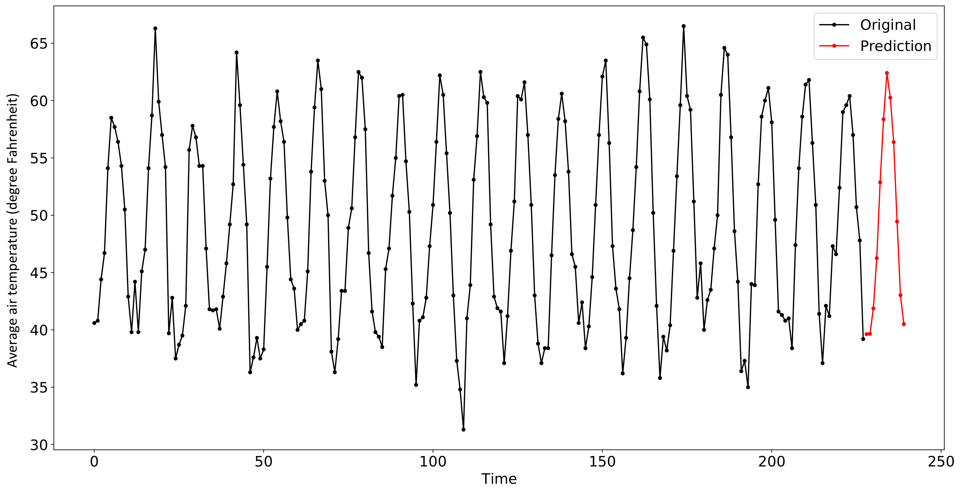
The model and predictions can be plotted using the psf_plot() function (shown in Listing 6) as shown in Figure 3.

Listing 6. Command to plot the original and predicted values

>>> psf_plot(a, b)

Listing 6. Command to plot the original and predicted values

>>> psf_plot(a, b)

A similar procedure was carried out to perform the prediction in R using the PSF library. Several error metrics was calculated for the predicted values and testing set. The performance of Python and R are compared in

Table 2. Comparison of forecast methods with different error metrics for the “nottem” dataset.

Function	Psf( )	Dpsf( )	psf( )	auto.arima( )
	(Python)	(Python)	(R)	(R)
Models	$(\mathit{k},\mathit{w})=(\mathbf{2},\mathbf{12})$	$(\mathit{k},\mathit{w})=(\mathbf{2},\mathbf{12})$	$(\mathit{k},\mathit{w})=(\mathbf{2},\mathbf{2})$	-
RMSE	1.84	5.27	2.24	2.34
MAE	1.54	4.77	1.94	1.93
MAPE	3.23	9.43	4.14	4.21
NSE	0.94	0.59	0.92	0.91

and Figure 4.

4.2. Example 2: CO₂ Dataset

This example demonstrates the use of the DPSF algorithm. The dataset consisted of atmospheric concentrations of CO${}_2$ expressed in parts per million (ppm) and reported in the preliminary 1997 SIO manometric mole fraction scale [46]. The values for February, March, and April of 1964 were missing and were obtained by interpolating linearly between the values for January and May of 1964.

Table 3. Statistical characteristics of the “CO${}_2$” dataset.

Mean	Median	Min	Max	SD	Kurtosis	Skewness
337.1	335.2	313.2	366.8	14.96622	−1.223013	0.2419156

contains the statistical characteristics of the time series.

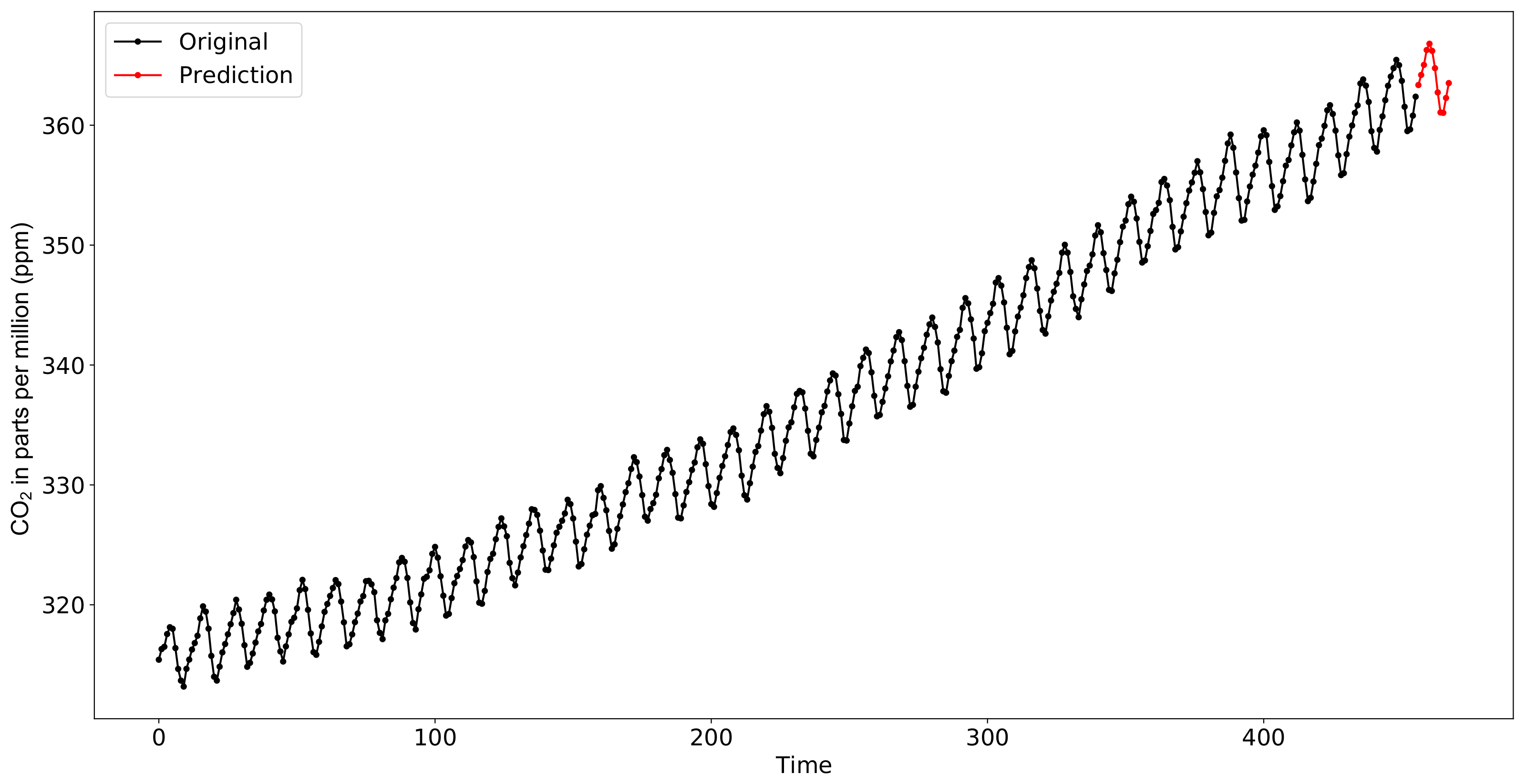
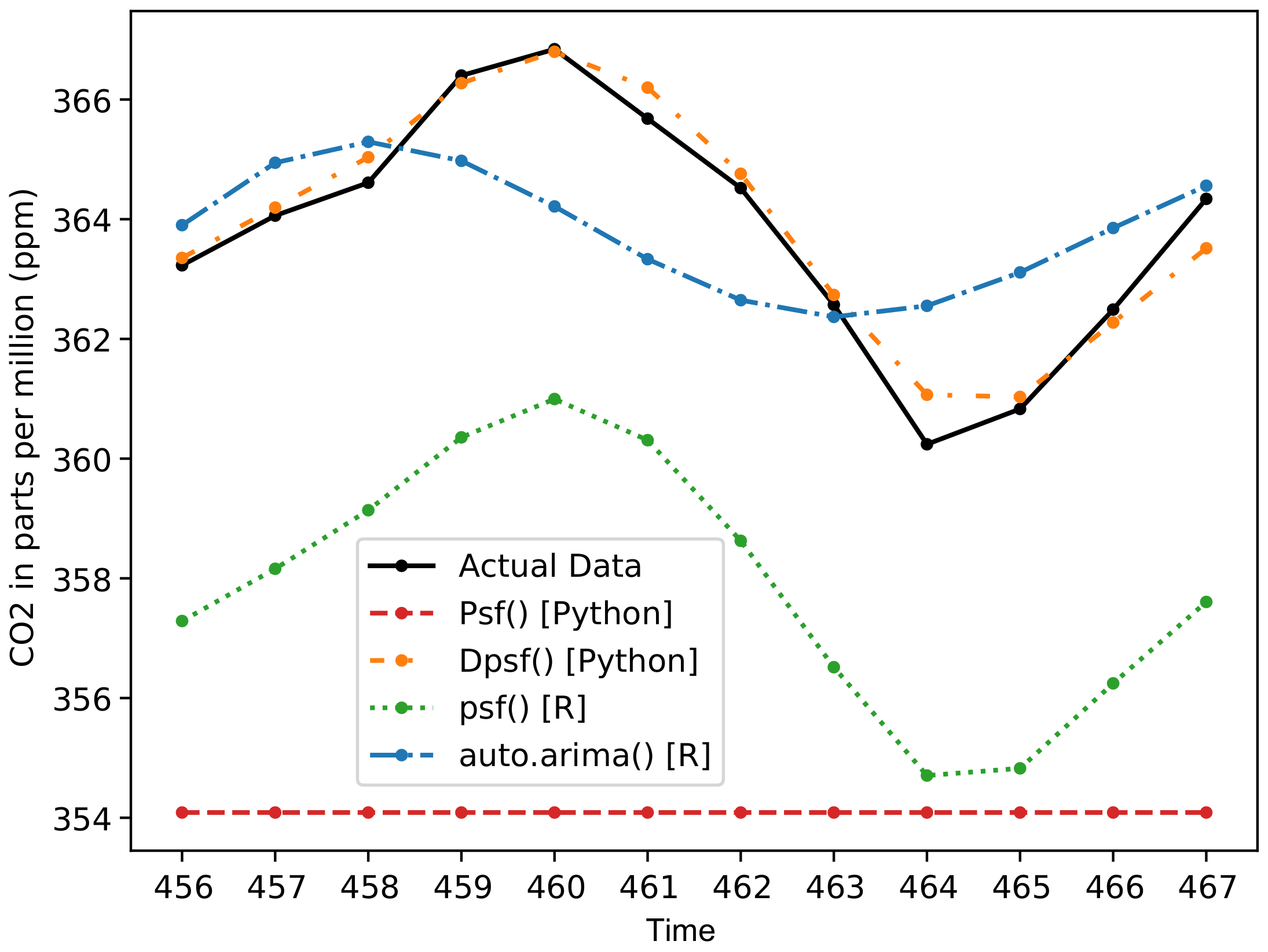
The time series data were divided into training and testing datasets. The training set contained the time series data, excluding the last 12 values. The testing dataset contained the last 12 values. A Dpsf model was created using the training dataset, and the future 12 values were forecasted as shown in Figure 5. The corresponding commands are shown in Listing 7. These predictions were then compared with the testing dataset. The comparisons are provided in

Table 4. Comparison of forecast methods with different error metrics for the “CO${}_2$” dataset.

Function	Dpsf( )	Psf( )	psf( )	auto.arima( )
	(Python)	(Python)	(R)	(R)
Models	$(\mathit{k},\mathit{w})=(\mathbf{2},\mathbf{18})$	$(\mathit{k},\mathit{w})=(\mathbf{9},\mathbf{19})$	$(\mathit{k},\mathit{w})=(\mathbf{2},\mathbf{10})$	-
RMSE	0.41	1.48	5.93	1.63
MAE	0.32	9.27	5.91	1.40
MAPE	0.08	2.67	1.62	0.38
NSE	0.95	0.32	−8.15	0.302

and Figure 6.

Listing 7. Command to create and use Dpsf model

# Import Dpsf, get_ts(), and dpsf_plot()
# from PSF_Py package
>>> from PSF_Py import Dpsf,dpsf_plot,get_ts
# Load the time series CO2
>>> ts = get_ts(’co2’)
# Divide the time series into training and testing
>>> train, test = ts[:len(ts)-12], ts[len(ts)-12:]
# Create Dpsf model
>>> a = Dpsf(data=train, cycle=12)
# The created model can be displayed using
# model_print() method
>>> a.model_print()
Original time-series :
0      315.42
1      316.31
2      316.50
3      317.56
4      318.13
5      318.00
6      316.39
7      314.65
8      313.68
9      313.18
10     314.66
\dots
448    365.45
449    365.01
450    363.70
451    361.54
452    359.51
453    359.65
454    360.80
455    362.38
Length: 456, dtype: float64
k =  2
w =  18
cycle =  12
dmin =  313.18
dmax =  365.45
type =  <class ’PSF_Py.dpsf.Dpsf’>
# Perform prediction using predict() method
>>> b = a.predict(n_ahead=12)
>>> b
array([363.35347826, 364.19434783, 365.03521739,
366.27304348, 366.79695652, 366.19913043, 364.75913043,
362.73458498, 361.06708498, 361.03143281, 362.2740415,
363.51445817])
# Plot the model and predicted values
>>> dpsf_plot(a,b)

Listing 7. Command to create and use Dpsf model

# Import Dpsf, get_ts(), and dpsf_plot()
# from PSF_Py package
>>> from PSF_Py import Dpsf,dpsf_plot,get_ts
# Load the time series CO2
>>> ts = get_ts(’co2’)
# Divide the time series into training and testing
>>> train, test = ts[:len(ts)-12], ts[len(ts)-12:]
# Create Dpsf model
>>> a = Dpsf(data=train, cycle=12)
# The created model can be displayed using
# model_print() method
>>> a.model_print()
Original time-series :
0      315.42
1      316.31
2      316.50
3      317.56
4      318.13
5      318.00
6      316.39
7      314.65
8      313.68
9      313.18
10     314.66
\dots
448    365.45
449    365.01
450    363.70
451    361.54
452    359.51
453    359.65
454    360.80
455    362.38
Length: 456, dtype: float64
k =  2
w =  18
cycle =  12
dmin =  313.18
dmax =  365.45
type =  <class ’PSF_Py.dpsf.Dpsf’>
# Perform prediction using predict() method
>>> b = a.predict(n_ahead=12)
>>> b
array([363.35347826, 364.19434783, 365.03521739,
366.27304348, 366.79695652, 366.19913043, 364.75913043,
362.73458498, 361.06708498, 361.03143281, 362.2740415,
363.51445817])
# Plot the model and predicted values
>>> dpsf_plot(a,b)

4.3. Example 3: Water Demand Dataset

The PSF and DPSF algorithms were applied to forecast water demand on the given dataset. Investigating such high complex time series data is highly important for water management [47].

Table 5. Statistical characteristics of the “Water Demand” dataset.

Mean	Median	Min	Max	SD	Kurtosis	Skewness
18.97	17.41	0.93	45.98	7.988099	0.3019151	0.6812421

contains the statistical characteristics of the time series.

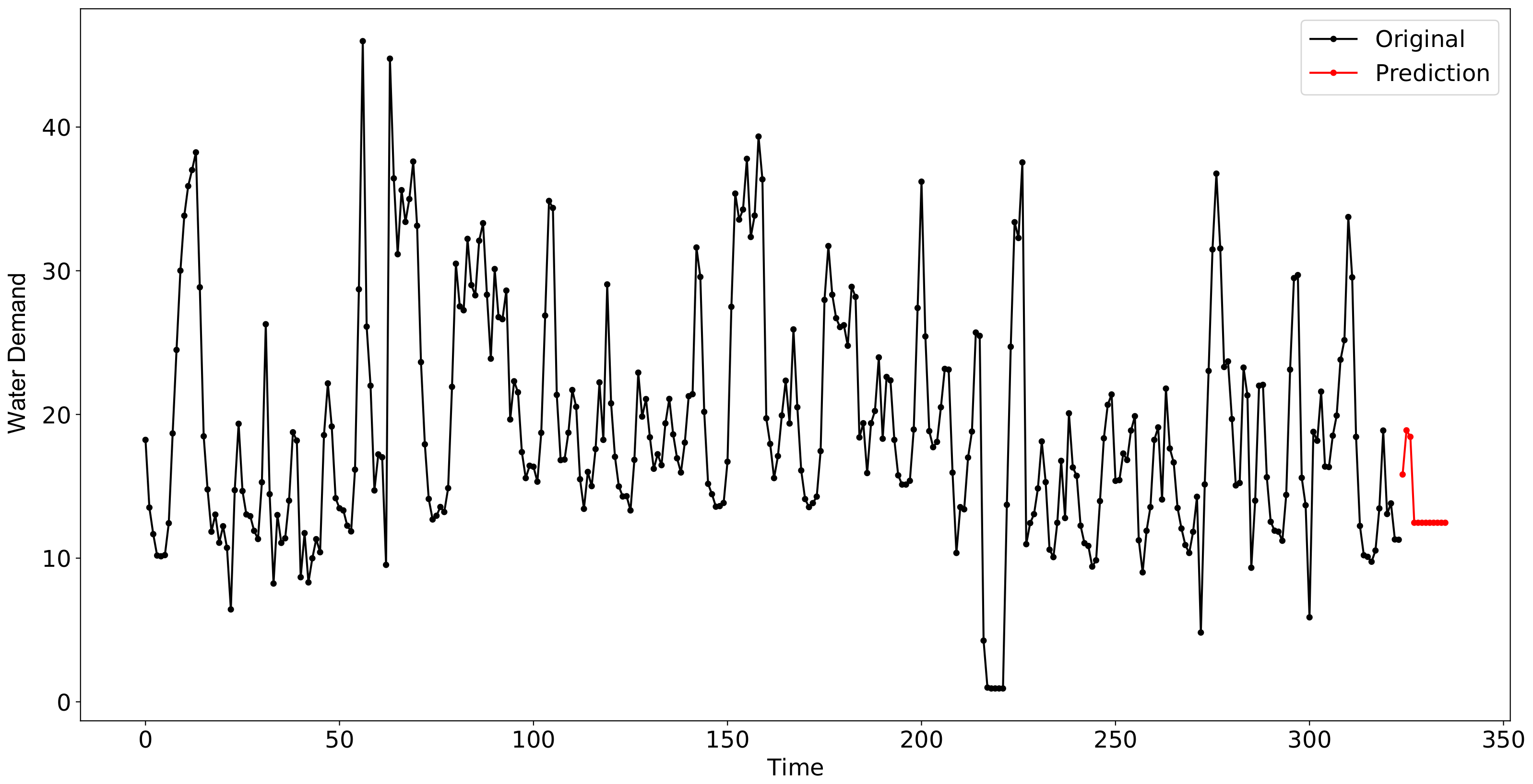
Different error metrics comparison is listed in

Table 6. Comparison of forecast methods with different error metrics for the “Water Demand” dataset.

Function	Dpsf( )	Psf( )	psf( )	auto.arima( )
	(Python)	(Python)	(R)	(R)
RMSE	6.16	5.92	6.45	7.55
MAE	4.98	4.37	5.07	5.93
MAPE	45.69	49.55	70.99	86.58
NSE	−1.79	−5.22	−0.17	−0.61

. The error for the Psf() function in python was found to be better than that of the other algorithms adopted in this study. The dataset and predictions using Psf() and Dpsf() are plotted in Figure 7 and Figure 8. Further, the comparison of forecasted values using various methods are shown in Figure 9.

4.4. Example 4: Total Solar Radiation Dataset

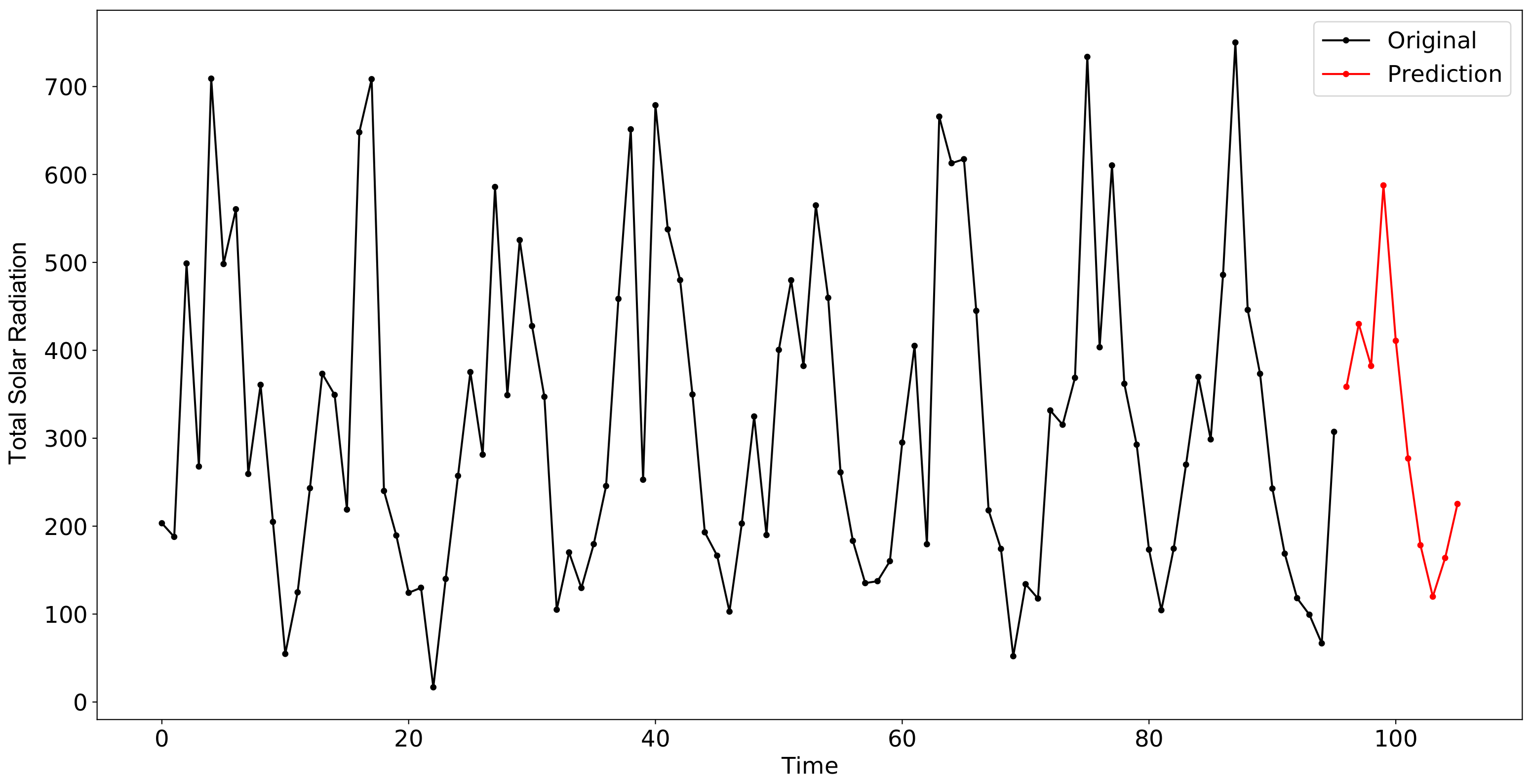
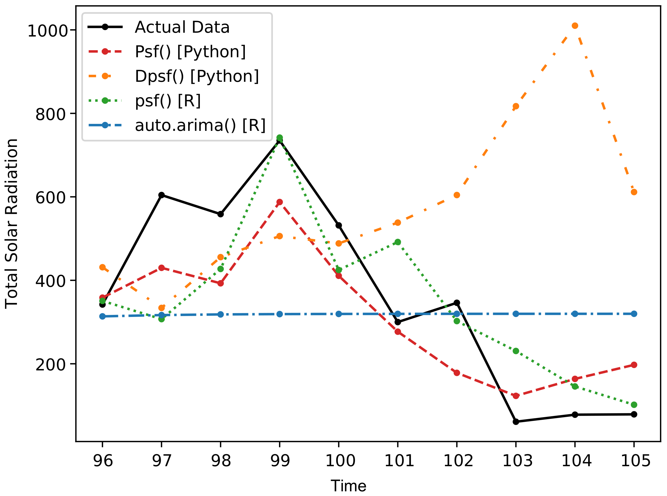
Among several climatological time series, total solar radiation is one of the essential climatological processes. Providing a robust soft-computing methodology for solar radiation can contribute remarkably to clean and friendly sources of energy [48]. The dataset consisted of daily solar radiation readings for year 2010 to year 2018 at Baker station in North Dakota. Before applying the algorithms, the dataset was reduced by taking the mean of the values for each month.

Table 7. Statistical characteristics of the “Total Solar Radiation” dataset.

Mean	Median	Min	Max	SD	Kurtosis	Skewness
325.11	296.90	16.71	750.09	188.0211	−0.7063935	0.5369928

presents the statistical characteristics of the time series. Performance of various methods are tabulated in

Table 8. Comparison of forecast methods with different error metrics for “Total Solar Radiation” dataset.

Function	Dpsf( )	Psf( )	psf( )	auto.arima( )
	(Python)	(Python)	(R)	(R)
RMSE	446.48	121.84	137.73	233.17
MAE	345.22	108.20	104.66	197.16
MAPE	338.73	52.37	56.56	124.71
NSE	−4.58	0.25	0.63	−0.043

. Results of psf_plot() and dpsf_plot() for the “Total Solar Radiation” dataset are shown in Figure 10 and Figure 11. Further, the comparison of forecasted values with different methods are shown in Figure 12.

The error for Psf() was significantly less the that for auto.arima() and Dpsf(). The errors are listed in Table 8.

4.5. Example 5: Average Bare Soil Temperature

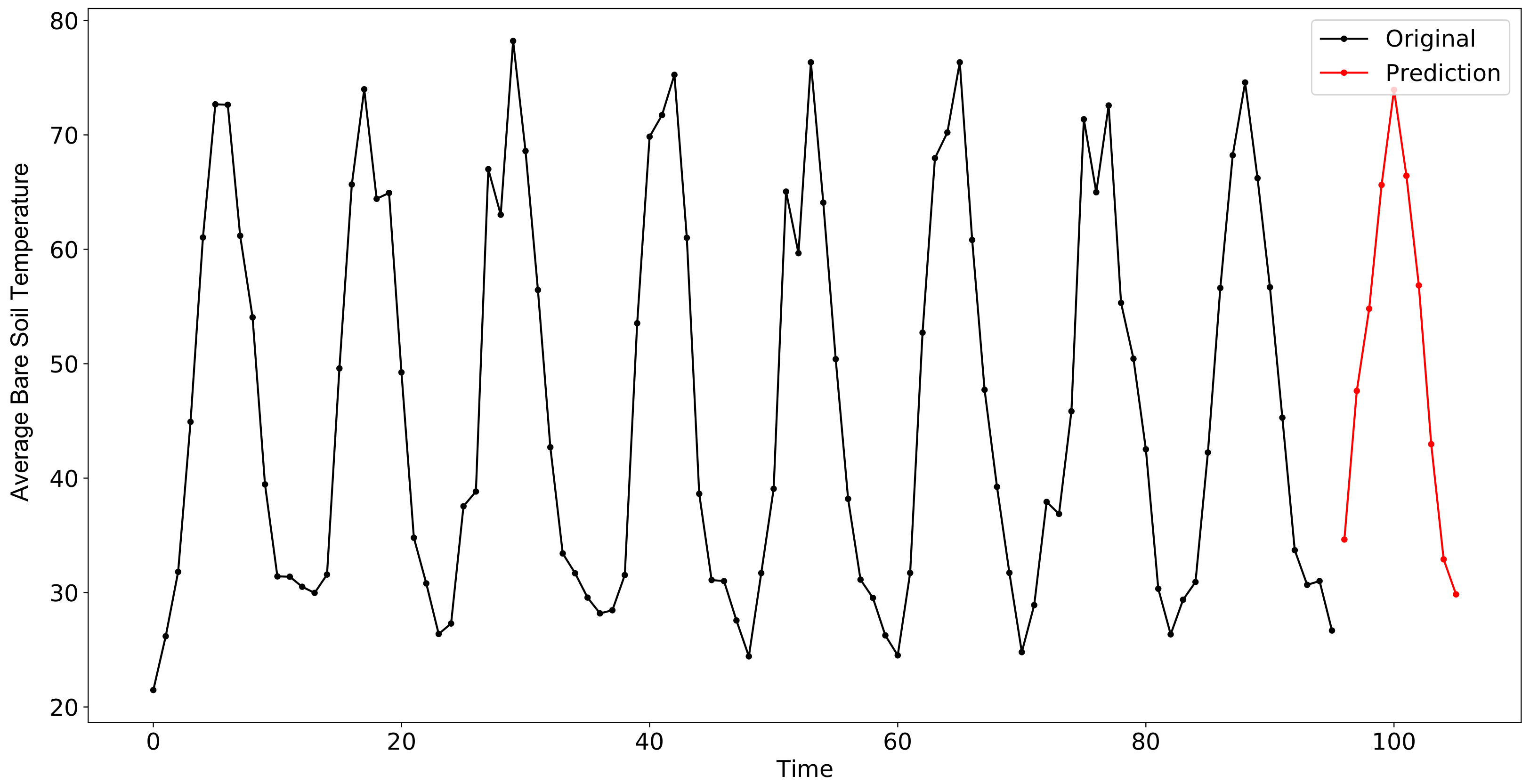
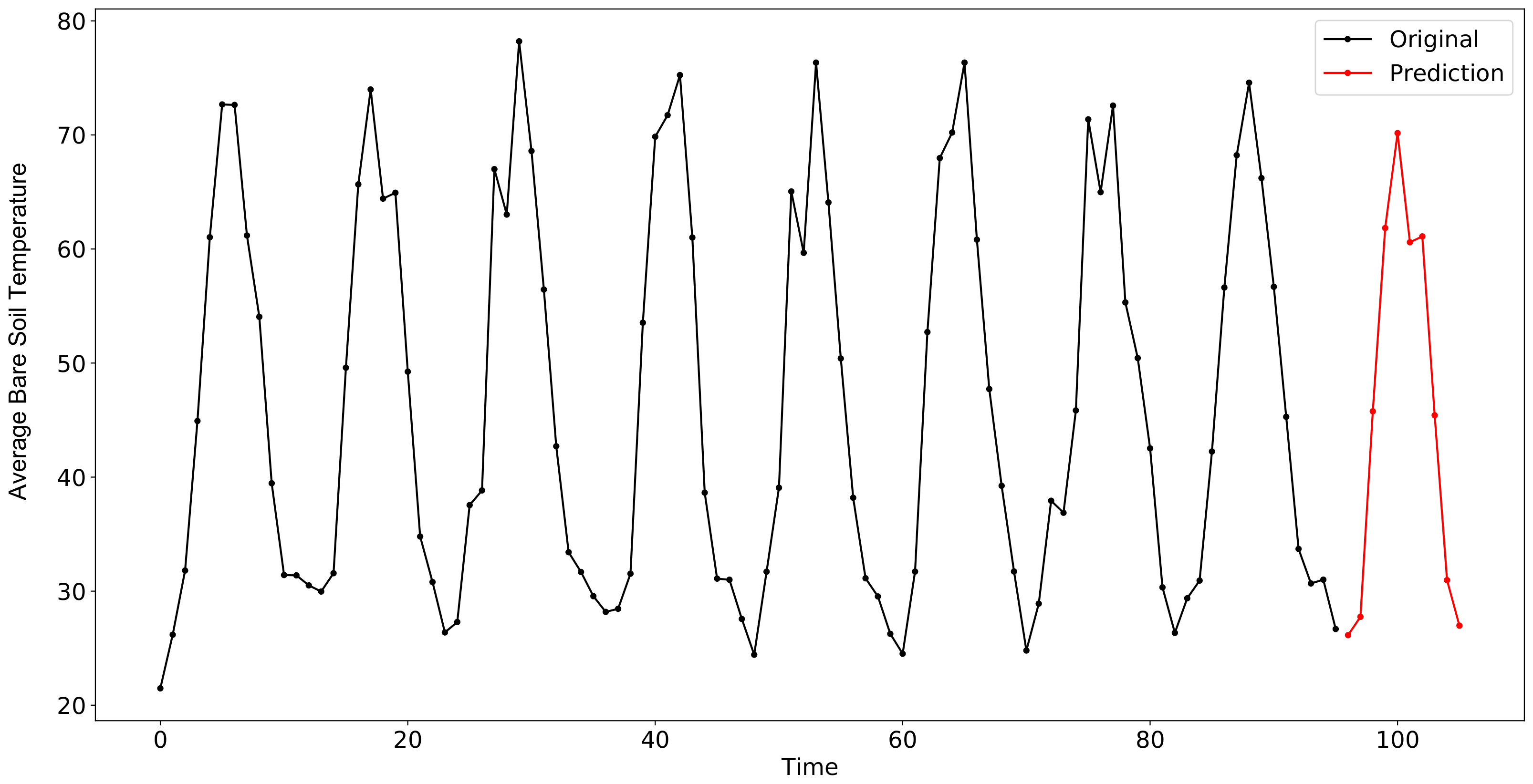
Soil temperature is an important process that is related to geoscience engineering [49]. Based on the factual mechanism, soil temperature has highly nonstationary features due to the influence of the soil morphology, climate, and hydrology information [50,51]. Hence, taking the soil temperature as a time series forecasting is highly useful for multiple geoscience engineering applications [52]. The data were obtained from the same region as in Example 4 (“Baker station”) and using the same data span, “2010–2018”. A similar modeling procedure was implemented as in Section 4.4.

Table 9. Statistical characteristics of the “Average Bare Soil Temperature”.

Mean	Median	Min	Max	SD	Kurtosis	Skewness
46.65	42.38	21.48	78.21	17.18163	−1.395386	0.355737

reports the statistical characteristics of the soil temperature time series, and the performance of various methods are tabulated in

Table 10. Comparison of forecast methods with different error metrics for the “Average Bare Soil Temperature” dataset.

Function	Dpsf( )	Psf( )	psf( )	auto.arima( )
	(Python)	(Python)	(R)	(R)
RMSE	12.70	7.92	9.38	8.75
MAE	9.40	5.79	7.69	7.32
MAPE	18.23	10.85	15.42	14.39
NSE	0.37	0.70	0.69	0.73

. Results of psf_plot() and dpsf_plot() for the “Average Bare Soil Temperature” dataset are shown in Figure 13 and Figure 14. Further, the comparison of forecasted values with different methods are shown in Figure 15.

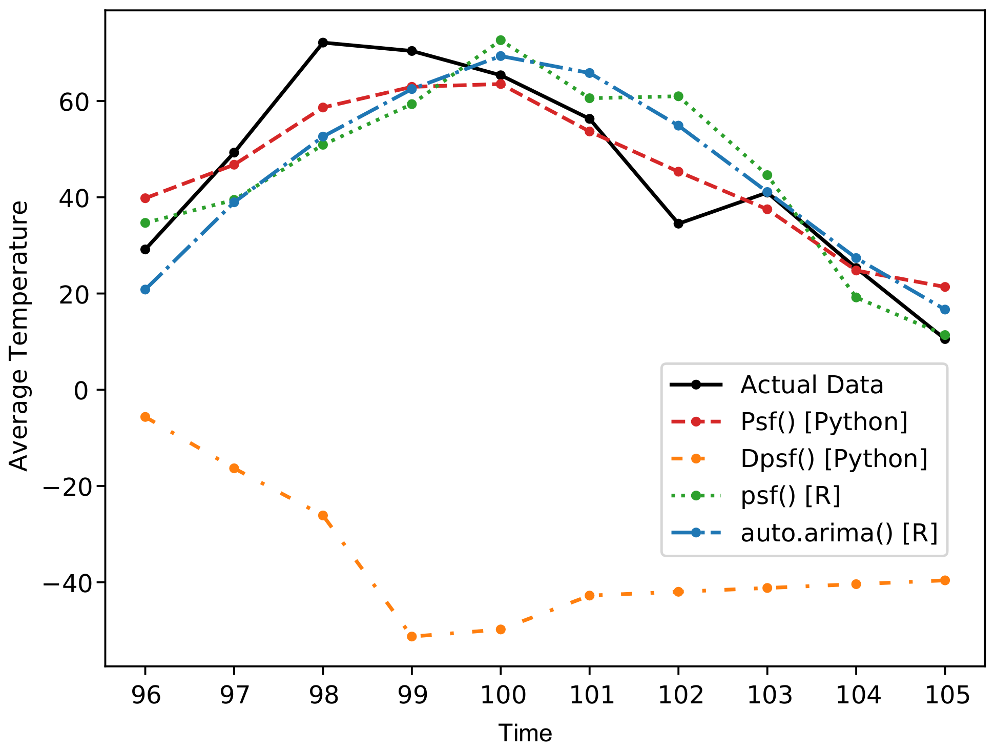
4.6. Example 6: Average Temperature

The final example reported in this research is modeling the air temperature. Having a reliable and robust technique for air temperature is very essential for diverse water resources and hydrological processes [53,54], for instance, in agriculture, water body evaporation, crops production, etc. [55]. Similar to Examples 4 and 5, the air temperature data were from the same station, region, and data span. For these data, the procedure followed was the same as in Examples 4 and 5.

Table 11. Statistical characteristics of the “Average Temperature” dataset.

Mean	Median	Min	Max	SD	Kurtosis	Skewness
39.48	43.47	−15.70	77.85	24.23293	−0.85042	−0.4995846

indicates the statistical characteristics of the time series. The performance of various methods are tabulated in

Table 12. Comparison of forecast methods with different error metrics for the “Average Temperature” dataset.

Function	Psf( )	Dpsf( )	psf( )	auto.arima( )
	(Python)	(Python)	(R)	(R)
RMSE	7.83	85.14	12.34	10.87
MAE	6.41	80.91	9.62	8.83
MAPE	22.29	207.16	22.03	22.03
NSE	0.69	−35.81	0.61	0.69

. Result of psf_plot() for the “Average Temperature” dataset are shown in Figure 16. Further, the comparison of forecasted values with different methods are shown in Figure 17.

5. Discussion and Conclusions

This paper described the PSF_Py package in detail and demonstrated its use for implementing the PSF and DPSF algorithms for diverse applications on real time series forecasting datasets. The package makes it very easy to make predictions using the PSF algorithm. The syntax is similar to that in R and is very easy to understand. The examples shown above suggested that the results from the Python package were comparable to those in R. The values of the window size and the number of clusters may differ in both packages. The algorithm worked exceptionally well for the time series containing periodic patterns. The forecasting error of the DPSF method, implemented in the proposed package, was much smaller and better than the benchmark ARIMA model. The complexity of a model is another critical aspect besides its accuracy. We compared the time and space complexities of the models in case studies with the GuessCompx tool. The GuessCompx tool [56,57] empirically estimates the computational complexity of a function in terms of Big-O notations. It computes multiple samples of increasing sizes from the given dataset and estimates the best-fit complexity according to the “leave-one-out mean squared error (LOO-MSE)” approach. The “nottem” dataset was used to calculate the complexities. The results of the tool are summarized in

Table 13. Estimated complexities according to the GuessCompx tool [56].

	Psf()(Python)/psf()(R)	Dpsf( ) (Python)	auto.arima( ) (R)
Time Complexity	$\mathcal{O}(logn)$	$\mathcal{O}(logn)$	$\mathcal{O}\left(n^3\right)$
Space Complexity	$\mathcal{O}(logn)$	$\mathcal{O}(logn)$	$\mathcal{O}\left(1\right)$

, and it shows that both PSF and DPSF models are computationally efficient and consumes an optimum amount of memory to achieve a better accuracy.

It is worth to mention that this research proposed a reliable and robust computational technique that can be implemented for online and offline forecasting for diverse hydrological and climatological applications [58,59]. In future work, other hybrid models [33,60] of the PSF method can be incorporated into the proposed Python package, with which further improved accuracy in forecasting can be targeted. In addition, the application of the proposed package could be extended to several new data-driven research domains. Further, other hydrological processes dataset or other engineering time series data could be investigated for the possibility to generalize the proposed package.

References

1. Faskari, S.A.; Ojim, G.; Falope, T.; Abdullahi, Y.B.; Abba, S. A Novel Machine Learning based Computing Algorithm in Modeling of Soiled Photovoltaic Module. Knowl. -Based Eng. Sci. 2022, 3, 28–36. [Google Scholar]
2. Bokde, N.; Feijóo, A.; Villanueva, D.; Kulat, K. A review on hybrid empirical mode decomposition models for wind speed and wind power prediction. Energies 2019, 12, 254. [Google Scholar] [CrossRef] [Green Version]
3. Bokde, N.; Feijóo, A.; Kulat, K. Analysis of differencing and decomposition preprocessing methods for wind speed prediction. Appl. Soft Comput. 2018, 71, 926–938. [Google Scholar] [CrossRef]
4. Cao, J.; Li, Z.; Li, J. Financial time series forecasting model based on CEEMDAN and LSTM. Phys. A Stat. Mech. Appl. 2019, 519, 127–139. [Google Scholar] [CrossRef]
5. Arce, P.; Antognini, J.; Kristjanpoller, W.; Salinas, L. Fast and Adaptive Cointegration Based Model for Forecasting High Frequency Financial Time Series. Comput. Econ. 2019, 54, 99–112. [Google Scholar] [CrossRef]
6. Shih, H.; Rajendran, S. Comparison of time series methods and machine learning algorithms for forecasting Taiwan Blood Services Foundation’s blood supply. J. Healthc. Eng. 2019, 2019, 6123745. [Google Scholar] [CrossRef]
7. Vázquez, M.; Melin, P.; Prado-Arechiga, G. Hybrid Neural-Fuzzy Modeling and Classification System for Blood Pressure Level Affectation. In Hybrid Intelligent Systems in Control, Pattern Recognition and Medicine; Springer: Berlin/Heidelberg, Germany, 2020; pp. 257–269. [Google Scholar]
8. Mithiya, D.; Datta, L.; Mandal, K. Time Series Analysis and Forecasting of Oilseeds Production in India: Using Autoregressive Integrated Moving Average and Group Method of Data Handling–Neural Network. Asian J. Agric. Ext. Econ. Sociol. 2019, 30, 1–14. [Google Scholar] [CrossRef] [Green Version]
9. Paliwal, V.; Ghare, A.D.; Mirajkar, A.B.; Bokde, N.D.; Feijoo Lorenzo, A.E. Computer Modeling for the Operation Optimization of Mula Reservoir, Upper Godavari Basin, India, Using the Jaya Algorithm. Sustainability 2020, 12, 84. [Google Scholar] [CrossRef] [Green Version]
10. Nguyen-Huy, T.; Deo, R.C.; Khan, S.; Devi, A.; Adeyinka, A.A.; Apan, A.A.; Yaseen, Z.M. Student Performance Predictions for Advanced Engineering Mathematics Course With New Multivariate Copula Models. IEEE Access 2022, 10, 45112–45136. [Google Scholar] [CrossRef]
11. Li, M.; Hinnov, L.; Kump, L. Acycle: Time-series analysis software for paleoclimate research and education. Comput. Geosci. 2019, 127, 12–22. [Google Scholar] [CrossRef]
12. Gonzalez-Vidal, A.; Jimenez, F.; Gomez-Skarmeta, A.F. A methodology for energy multivariate time series forecasting in smart buildings based on feature selection. Energy Build. 2019, 196, 71–82. [Google Scholar] [CrossRef]
13. Gupta, A.; Bokde, N.; Kulat, K. Hybrid leakage management for water network using PSF algorithm and soft computing techniques. Water Resour. Manag. 2018, 32, 1133–1151. [Google Scholar] [CrossRef]
14. Kim, J.; Lee, H. A study on predictive model for forecasting anti-aircraft missile spare parts demand based on machine learning. Korean Data Inf. Sci. Soc. 2019, 30, 587–596. [Google Scholar]
15. Bokde, N.; Beck, M.W.; Álvarez, F.M.; Kulat, K. A novel imputation methodology for time series based on pattern sequence forecasting. Pattern Recognit. Lett. 2018, 116, 88–96. [Google Scholar] [CrossRef]
16. Arikan, B.B.; Jiechen, L.; Sabbah, I.I.; Ewees, A.; Homsi, R.; Sulaiman, S.O. Dew Point Time Series Forecasting at the North Dakota. Knowl. -Based Eng. Sci. 2021, 2, 24–34. [Google Scholar] [CrossRef]
17. Cui, F.; Salih, S.Q.; Choubin, B.; Bhagat, S.K.; Samui, P.; Yaseen, Z.M. Newly explored machine learning model for river flow time series forecasting at Mary River, Australia. Environ. Monit. Assess. 2020, 192, 1–15. [Google Scholar] [CrossRef]
18. Bokde, N.D.; Feijóo, A.; Al-Ansari, N.; Yaseen, Z.M. A comparison between reconstruction methods for generation of synthetic time series applied to wind speed simulation. IEEE Access 2019, 7, 135386–135398. [Google Scholar] [CrossRef]
19. De Gooijer, J.G.; Hyndman, R.J. 25 years of time series forecasting. Int. J. Forecast. 2006, 22, 443–473. [Google Scholar] [CrossRef] [Green Version]
20. Zhang, G.P. Time series forecasting using a hybrid ARIMA and neural network model. Neurocomputing 2003, 50, 159–175. [Google Scholar] [CrossRef]
21. Hu, H.; Zhang, J.; Li, T. A Comparative Study of VMD-Based Hybrid Forecasting Model for Nonstationary Daily Streamflow Time Series. Complexity 2020, 2020, 4064851. [Google Scholar] [CrossRef]
22. Alvarez, F.M.; Troncoso, A.; Riquelme, J.C.; Ruiz, J.S.A. Energy time series forecasting based on pattern sequence similarity. IEEE Trans. Knowl. Data Eng. 2010, 23, 1230–1243. [Google Scholar] [CrossRef]
23. Jin, C.H.; Pok, G.; Park, H.W.; Ryu, K.H. Improved pattern sequence-based forecasting method for electricity load. IEEJ Trans. Electr. Electron. Eng. 2014, 9, 670–674. [Google Scholar] [CrossRef]
24. Shen, W.; Babushkin, V.; Aung, Z.; Woon, W.L. An ensemble model for day-ahead electricity demand time series forecasting. In Proceedings of the Fourth International Conference on Future Energy Systems, ACM, Berkeley, CA, USA, 21–24 May 2013; pp. 51–62. [Google Scholar]
25. Koprinska, I.; Rana, M.; Troncoso, A.; Martínez-Álvarez, F. Combining pattern sequence similarity with neural networks for forecasting electricity demand time series. In Proceedings of the 2013 International Joint Conference on Neural Networks (IJCNN), Dallas, TX, USA, 4–9 August 2013; pp. 1–8. [Google Scholar]
26. Fujimoto, Y.; Hayashi, Y. Pattern sequence-based energy demand forecast using photovoltaic energy records. In Proceedings of the 2012 International Conference on Renewable Energy Research and Applications (ICRERA), Nagasaki, Japan, 11–14 November 2012; pp. 1–6. [Google Scholar]
27. Bokde, N.; Asencio-Cortés, G.; Martínez-Álvarez, F.; Kulat, K. PSF: Introduction to R Package for Pattern Sequence Based Forecasting Algorithm. R J. 2017, 9, 324–333. [Google Scholar] [CrossRef] [Green Version]
28. Bokde, N.; Asencio-Cortés, G.; Martínez-Álvarez, F. PSF: Forecasting of Univariate Time Series Using the Pattern Sequence-Based Forecasting (PSF) Algorithm, R Package Version 0.4; R Foundation for Statistical Computing: Vienna, Austria, 2017. [Google Scholar]
29. Bokde, N.; Troncoso, A.; Asencio-Cortés, G.; Kulat, K.; Martínez-Álvarez, F. Pattern sequence similarity based techniques for wind speed forecasting. In Proceedings of the International Work-Conference on Time Series (ITISE), Granada, Spain, 27–29 June 2017; pp. 18–20. [Google Scholar]
30. Bokde, N.; Tranberg, B.; Andresen, G.B. A graphical approach to carbon-efficient spot market scheduling for Power-to-X applications. Energy Convers. Manag. 2020, 224, 113461. [Google Scholar] [CrossRef]
31. Bokde, N.D.; Tranberg, B.; Andresen, G.B. Short-term CO2 emissions forecasting based on decomposition approaches and its impact on electricity market scheduling. Appl. Energy 2021, 281, 116061. [Google Scholar] [CrossRef]
32. Patil, J.; Bokde, N.; Mishra, S.K.; Kulat, K. PSF-Based Spectrum Occupancy Prediction in Cognitive Radio. In Advanced Engineering Optimization Through Intelligent Techniques; Springer: Berlin/Heidelberg, Germany, 2020; pp. 609–619. [Google Scholar]
33. Bokde, N.; Feijóo, A.; Al-Ansari, N.; Tao, S.; Yaseen, Z.M. The hybridization of ensemble empirical mode decomposition with forecasting models: Application of short-term wind speed and power modeling. Energies 2020, 13, 1666. [Google Scholar] [CrossRef] [Green Version]
34. Song, T.; Ding, W.; Liu, H.; Wu, J.; Zhou, H.; Chu, J. Uncertainty Quantification in Machine Learning Modeling for Multi-Step Time Series Forecasting: Example of Recurrent Neural Networks in Discharge Simulations. Water 2020, 12, 912. [Google Scholar] [CrossRef] [Green Version]
35. Niu, W.J.; Feng, Z.K.; Chen, Y.B.; Zhang, H.R.; Cheng, C.T. Annual streamflow time series prediction using extreme learning machine based on gravitational search algorithm and variational mode decomposition. J. Hydrol. Eng. 2020, 25, 04020008. [Google Scholar] [CrossRef]
36. Mazher, A. Visualization Framework for High-Dimensional Spatio-Temporal Hydrological Gridded Datasets using Machine-Learning Techniques. Water 2020, 12, 590. [Google Scholar] [CrossRef] [Green Version]
37. PSF_Py. Python Package Version 0.1. Available online: https://pypi.org/project/PSF-Py/ (accessed on 1 December 2021).
38. GitHub PSF_Py. Available online: https://github.com/Mayur1009/PSF_py (accessed on 31 December 2019).
39. Hyndman, R.J.; Khandakar, Y. Automatic Time Series for Forecasting: The Forecast Package for R; Number 6/07; Department of Econometrics and Business Statistics, Monash University: Victoria, Australia, 2007. [Google Scholar]
40. Charte, F.; Vico, A.; Pérez-Godoy, M.D.; Rivera, A.J. predtoolsTS: R package for streamlining time series forecasting. Prog. Artif. Intell. 2019, 8, 505–510. [Google Scholar] [CrossRef]
41. Bokde, N.D.; Yaseen, Z.M.; Andersen, G.B. ForecastTB—An R Package as a Test-Bench for Time Series Forecasting—Application of Wind Speed and Solar Radiation Modeling. Energies 2020, 13, 2578. [Google Scholar] [CrossRef]
42. Shende, M.K.; Feijóo-Lorenzo, A.E.; Bokde, N.D. cleanTS: Automated (AutoML) tool to clean univariate time series at microscales. Neurocomputing 2022, 500, 155–176. [Google Scholar] [CrossRef]
43. Omeje, O.E.; Maccido, H.S.; Badamasi, Y.A.; Abba, S.I. Performance of Hybrid Neuro-Fuzzy Model for Solar Radiation Simulation at Abuja, Nigeria: A Correlation Based Input Selection Technique. Knowl.-Based Eng. Sci. 2021, 2, 54–66. [Google Scholar]
44. Yaseen, Z.M. An insight into machine learning models era in simulating soil, water bodies and adsorption heavy metals: Review, challenges and solutions. Chemosphere 2021, 277, 130126. [Google Scholar] [CrossRef]
45. Anderson, O. The Box-Jenkins approach to time series analysis. RAIRO -Oper. Res. 1977, 11, 3–29. [Google Scholar] [CrossRef] [Green Version]
46. Keeling, C.D.; Whorf, T.P.; Scripps Institution of Oceanogra-phy (SIO) University of California, La Jolla. Data 2000. Available online: http://cdiac.esd.ornl.gov/trends/co2/sio-mlo.htm (accessed on 1 December 2021).
47. Abd Rahman, N.; Muhammad, N.S.; Abdullah, J.; Wan Mohtar, W.H.M. Model performance indicator of aging pipes in a domestic water supply distribution network. Water 2019, 11, 2378. [Google Scholar] [CrossRef] [Green Version]
48. Sharafati, A.; Khosravi, K.; Khosravinia, P.; Ahmed, K.; Salman, S.A.; Yaseen, Z.M.; Shahid, S. The potential of novel data mining models for global solar radiation prediction. Int. J. Environ. Sci. Technol. 2019, 16, 7147–7164. [Google Scholar] [CrossRef]
49. Razali, S.F.M.; Wahab, J.A.; Mukhlisin, M.; Arshad, I.; Mohamed, Z.S. Effectiveness of Electrical Capacitance Volume Tomography Method in Soil Water Content Measurement. J. Teknol. 2013, 65, 55–59. [Google Scholar]
50. Guo, L.; Fu, P.; Shi, T.; Chen, Y.; Zhang, H.; Meng, R.; Wang, S. Mapping field-scale soil organic carbon with unmanned aircraft system-acquired time series multispectral images. Soil Tillage Res. 2020, 196, 104477. [Google Scholar] [CrossRef]
51. Penghui, L.; Ewees, A.A.; Beyaztas, B.H.; Qi, C.; Salih, S.Q.; Al-Ansari, N.; Bhagat, S.K.; Yaseen, Z.M.; Singh, V.P. Metaheuristic Optimization Algorithms Hybridized With Artificial Intelligence Model for Soil Temperature Prediction: Novel Model. IEEE Access 2020, 8, 51884–51904. [Google Scholar] [CrossRef]
52. Wei, X.; Zhang, L.; Yang, H.Q.; Zhang, L.; Yao, Y.P. Machine learning for pore-water pressure time-series prediction: Application of recurrent neural networks. Geosci. Front. 2020, 12, 453–467. [Google Scholar] [CrossRef]
53. Naganna, S.R.; Deka, P.C.; Ghorbani, M.A.; Biazar, S.M.; Al-Ansari, N.; Yaseen, Z.M. Dew point temperature estimation: Application of artificial intelligence model integrated with nature-inspired optimization algorithms. Water 2019, 11, 742. [Google Scholar] [CrossRef] [Green Version]
54. Nearing, G.S.; Kratzert, F.; Sampson, A.K.; Pelissier, C.S.; Klotz, D.; Frame, J.M.; Prieto, C.; Gupta, H.V. What role does hydrological science play in the age of machine learning? Water Resour. Res. 2020, 57, e2020WR028091. [Google Scholar] [CrossRef]
55. Azad, A.; Kashi, H.; Farzin, S.; Singh, V.P.; Kisi, O.; Karami, H.; Sanikhani, H. Novel approaches for air temperature prediction: A comparison of four hybrid evolutionary fuzzy models. Meteorol. Appl. 2020, 27, e1817. [Google Scholar] [CrossRef] [Green Version]
56. Agenis-Nevers, M.; Bokde, N.D.; Yaseen, Z.M.; Shende, M.K. An empirical estimation for time and memory algorithm complexities: Newly developed R package. Multimed. Tools Appl. 2021, 80, 2997–3015. [Google Scholar] [CrossRef]
57. Agenis, M.; Bokde, N. GuessCompx: Empirically Estimates Algorithm Complexity; R Package Version 1.0.3; R Foundation for Statistical Computing: Vienna, Austria, 2019. [Google Scholar]
58. Ozkan, M.B.; Karagoz, P. Data mining-based upscaling approach for regional wind power forecasting: Regional statistical hybrid wind power forecast technique (RegionalSHWIP). IEEE Access 2019, 7, 171790–171800. [Google Scholar] [CrossRef]
59. Zsoter, E.; Cloke, H.; Stephens, E.; de Rosnay, P.; Muñoz-Sabater, J.; Prudhomme, C.; Pappenberger, F. How well do operational Numerical Weather Prediction configurations represent hydrology? J. Hydrometeorol. 2019, 20, 1533–1552. [Google Scholar] [CrossRef]
60. Bokde, N.; Feijóo, A.; Villanueva, D.; Kulat, K. A Novel and Alternative Approach for Direct and Indirect Wind-Power Prediction Methods. Energies 2018, 11, 2923. [Google Scholar] [CrossRef] [Green Version]
Figure 1. Block diagram of the PSF method (Source: [33]).
Applsci 12 06194 g001
Figure 2. Prediction with PSF algorithm (Source: [27]).
Applsci 12 06194 g002
Figure 3. Result of psf_plot() for the “nottem” dataset.
Applsci 12 06194 g003
Figure 4. Plot showing the test data and values forecasted using various methods for the “nottem” dataset.
Applsci 12 06194 g004
Figure 5. Result of dpsf_plot() for the “CO 2 ” dataset.
Applsci 12 06194 g005
Figure 6. Plot showing the test data and values forecasted using various methods for the “CO 2 ” dataset.
Applsci 12 06194 g006
Figure 7. Result of psf_plot() for the “Water Demand” dataset.
Applsci 12 06194 g007
Figure 8. Result of dpsf_plot() for the “Water Demand” dataset.
Applsci 12 06194 g008
Figure 9. Plot showing the test data and values forecasted using various methods for the “Water Demand” dataset.
Applsci 12 06194 g009
Figure 10. Result of psf_plot() for the “Total Solar Radiation” dataset.
Applsci 12 06194 g010
Figure 11. Result of dpsf_plot() for the “Total Solar Radiation” dataset.
Applsci 12 06194 g011
Figure 12. Plot showing the test data and values forecasted using various methods for the “Total Solar Radiation” dataset.
Applsci 12 06194 g012
Figure 13. Result of psf_plot() for the “Average Bare Soil Temperature” dataset.
Applsci 12 06194 g013
Figure 14. Result of dpsf_plot() for the “Average Bare Soil Temperature” dataset.
Applsci 12 06194 g014
Figure 15. Plot showing the test data and values forecasted using various methods for the “Average Bare Soil Temperature” dataset.
Applsci 12 06194 g015
Figure 16. Plot showing result of psf_plot() for the “Average Temperature” dataset.
Applsci 12 06194 g016
Figure 17. Plot showing the test data and values forecasted using various methods for the “Average Temperature” dataset.
Applsci 12 06194 g017