
Estimation of Blast-Induced Peak Particle Velocity through the Improved Weighted Random Forest Technique

 ,
,  ,
,  ,
,  and
and 
Abstract
:1. Introduction
2. Project Description and Data Collection
3. Methods
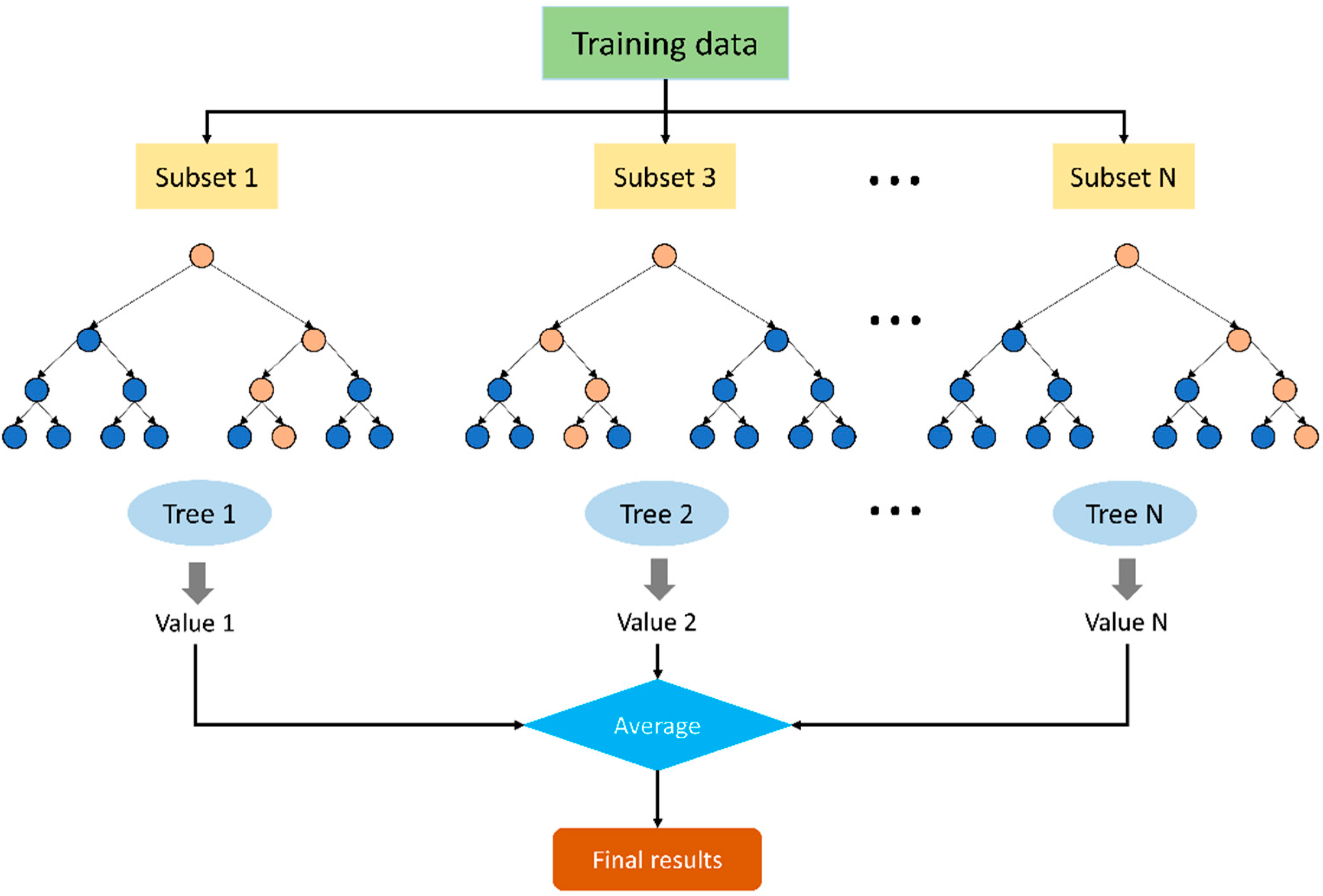
3.1. RF
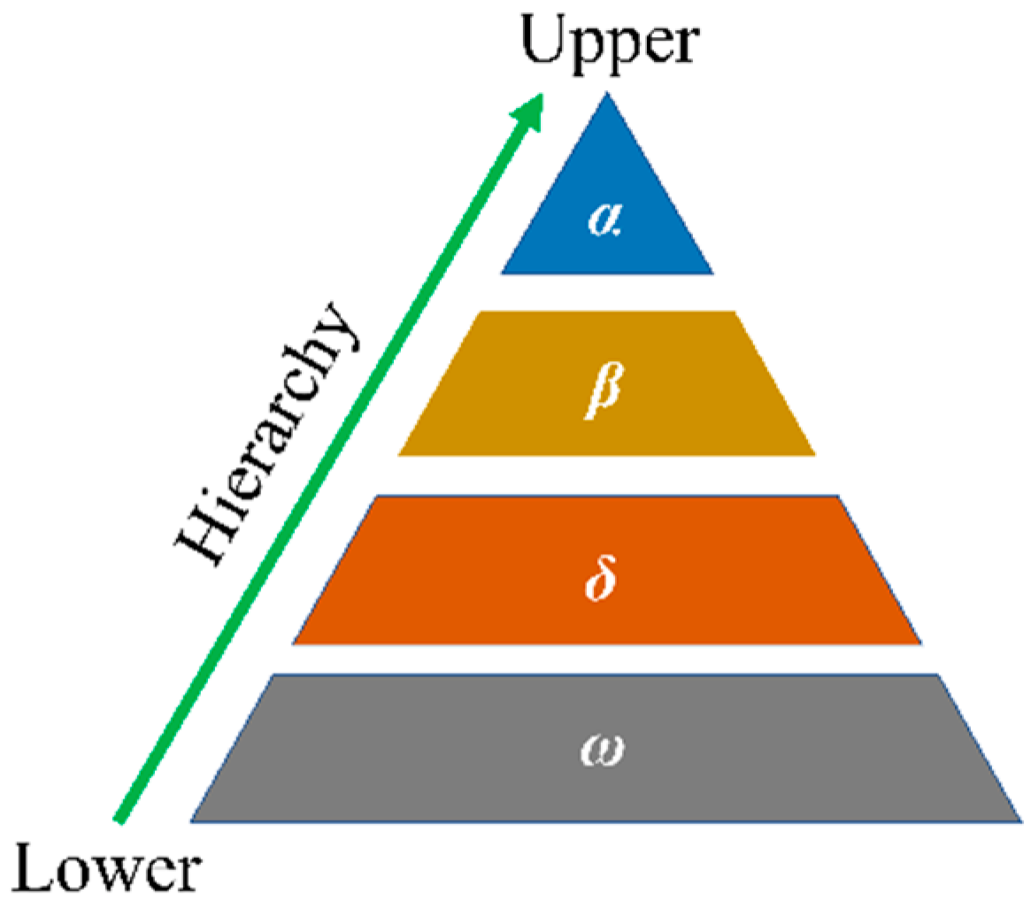
3.2. GWO
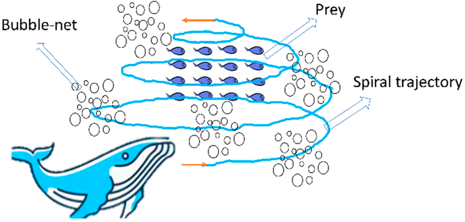
3.3. WOA
3.4. TSA
- (1)
- Initialization
- (2)
- Avoid conflicts between search agents
- (3)
- Move to the best neighbor
- (4)
- Move towards the best individual
- (5)
- Swarm behavior
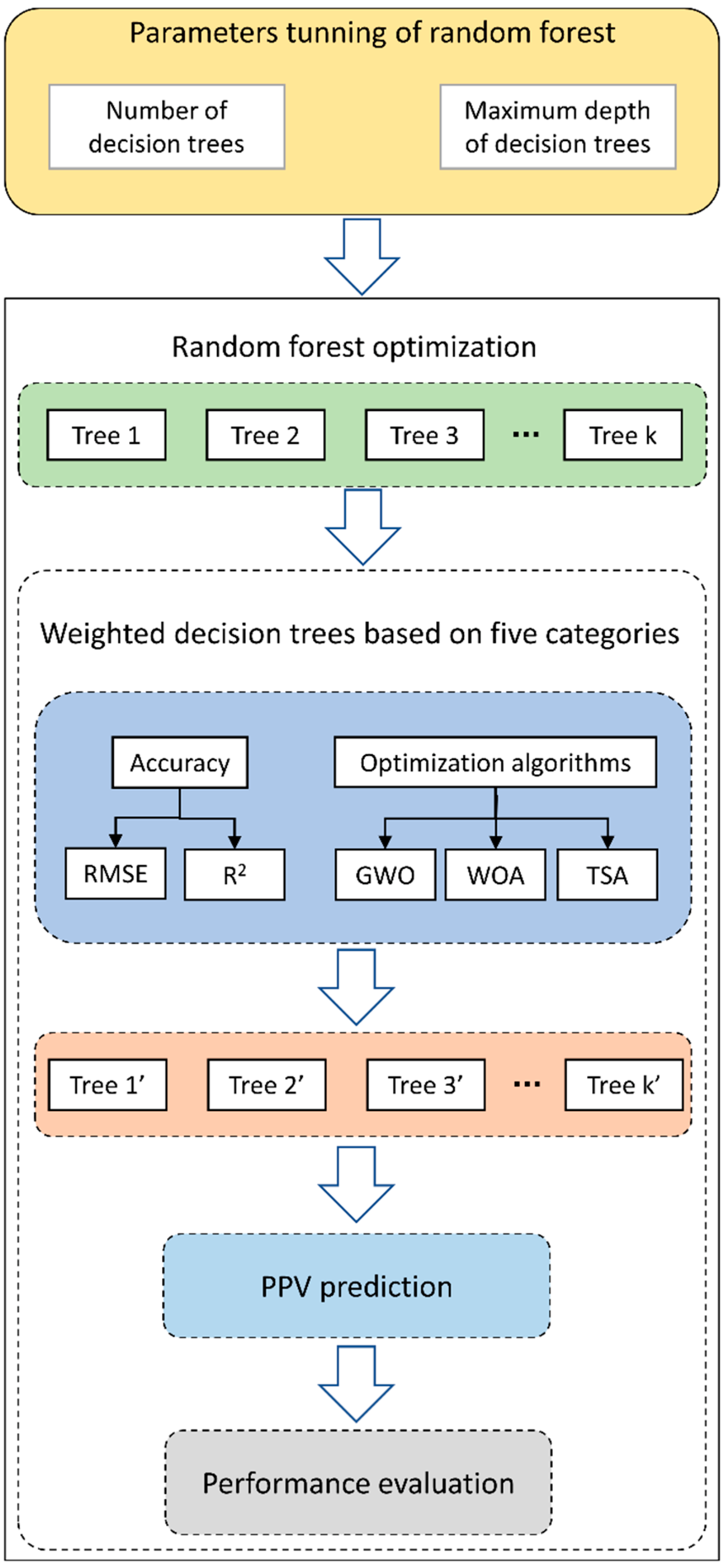
3.5. Improved RF Models
3.5.1. Improved Weights Based on the Accuracy
3.5.2. Improved Weights Based on Three Metaheuristic Algorithms
- (1)
- Data preparation: randomly divide the raw data into a training set (80% of raw data) and a testing set (20% of raw data);
- (2)
- Initialization: Initialize the swarm size, iterations, as well as some necessary parameters of the three optimization algorithms;
- (3)
- Fitness evaluation: Calculate the fitness value of the population, evaluate its fitness, and then save the best fitness value before starting the next iteration;
- (4)
- Update parameters: Update the fitness value based on the outcome of each iteration, which aims to capture the ideal solutions;
- (5)
- Suspension conditions check: When the optimal fitness value no longer changes, or the maximum number of iterations is reached, the optimal solutions of the weights of decision trees are obtained.
3.6. Criteria for Evaluation
4. Results and Discussion
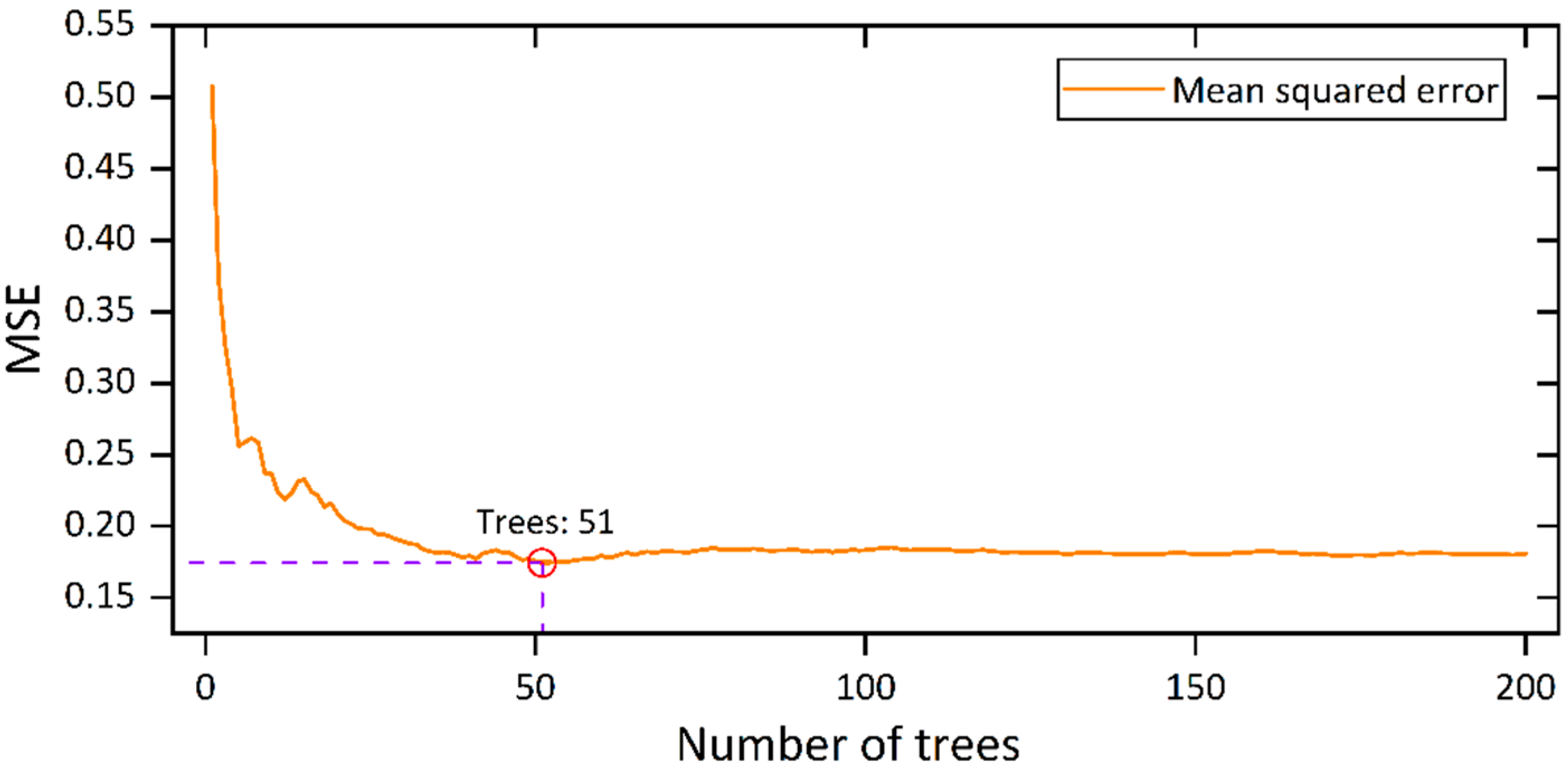
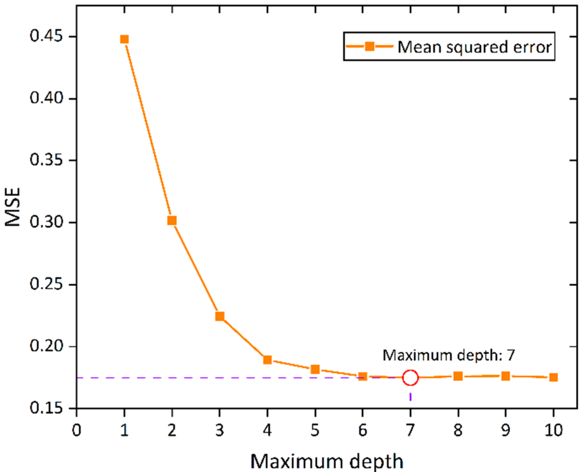
4.1. Parameter Tuning of the RF Model
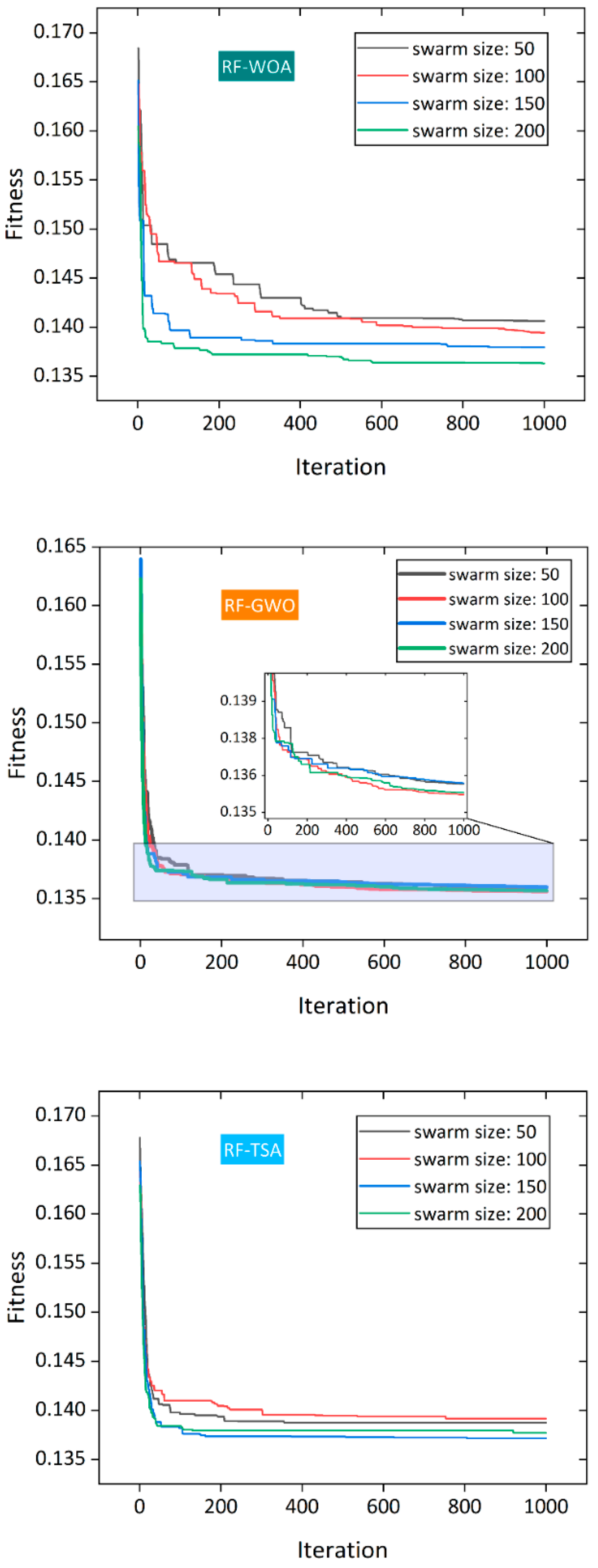
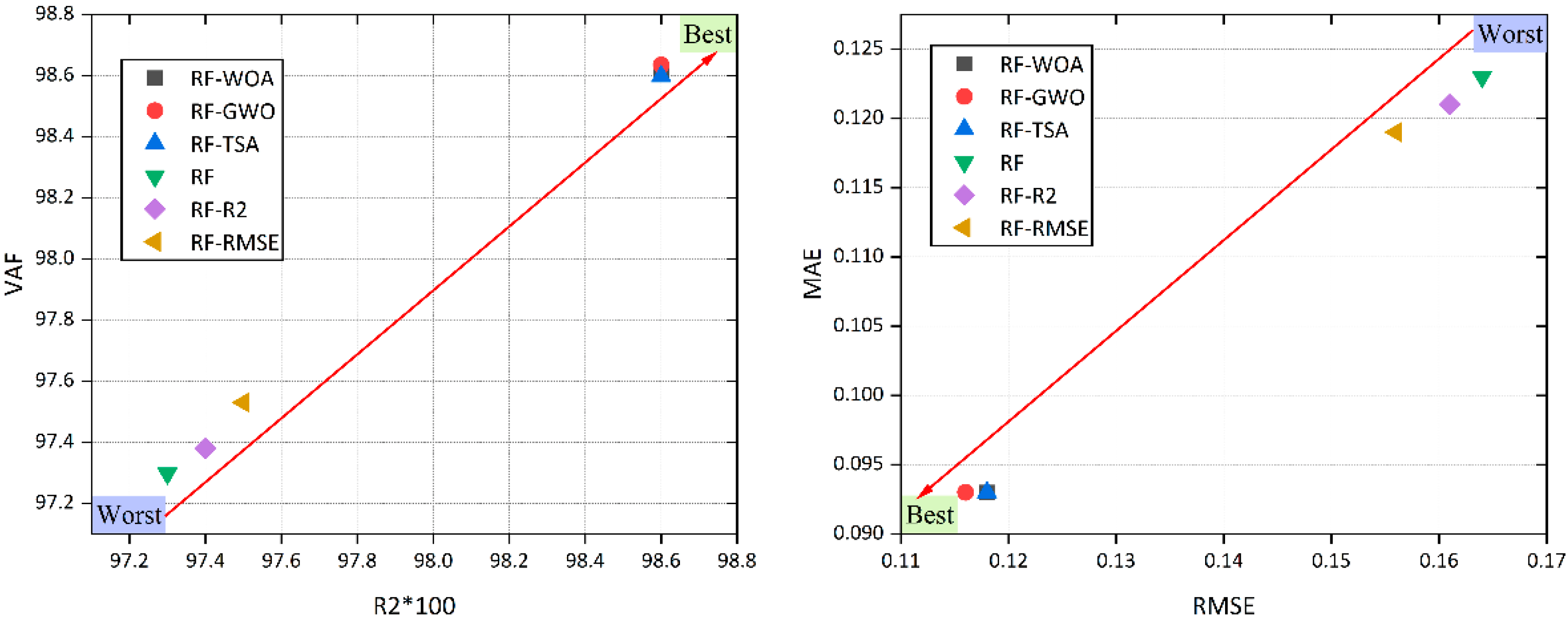
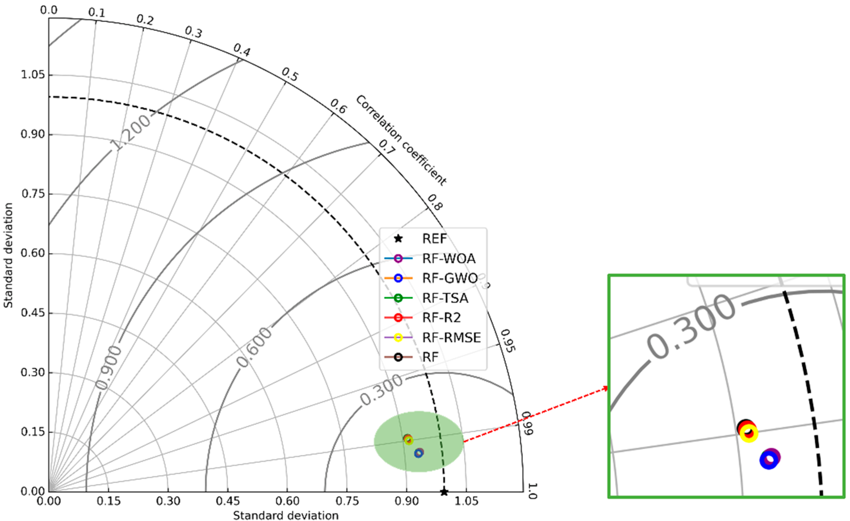
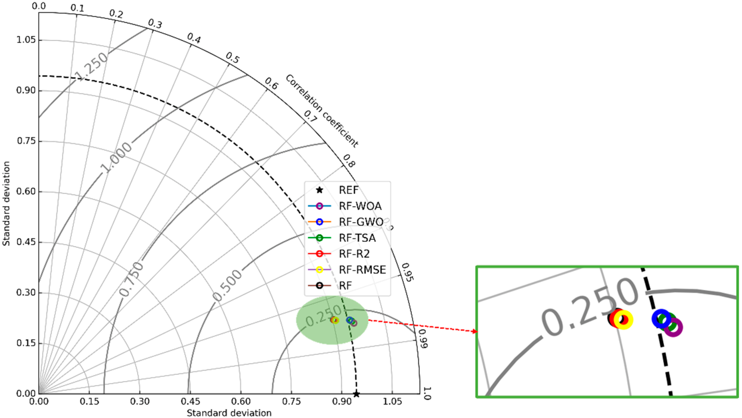
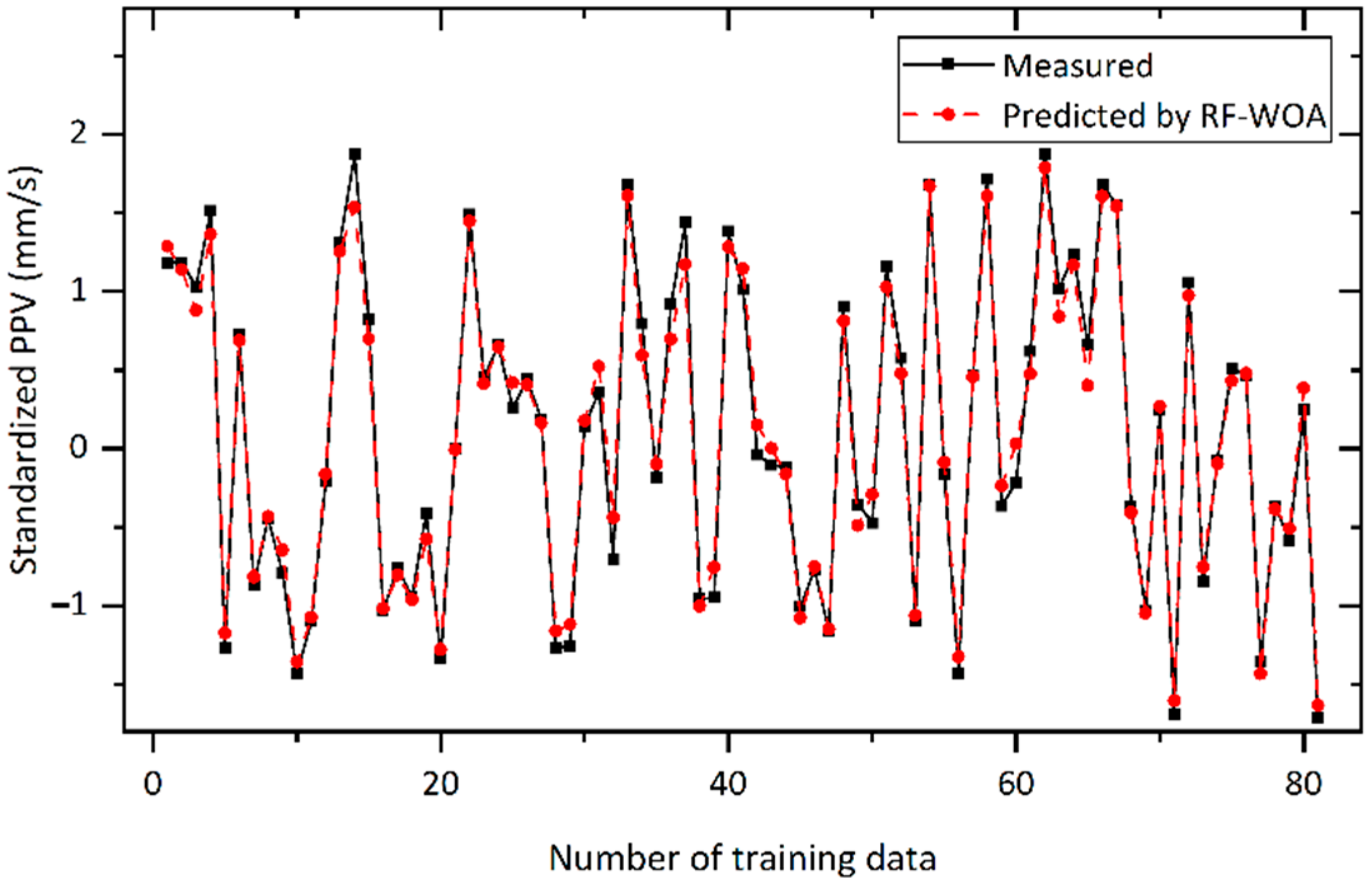
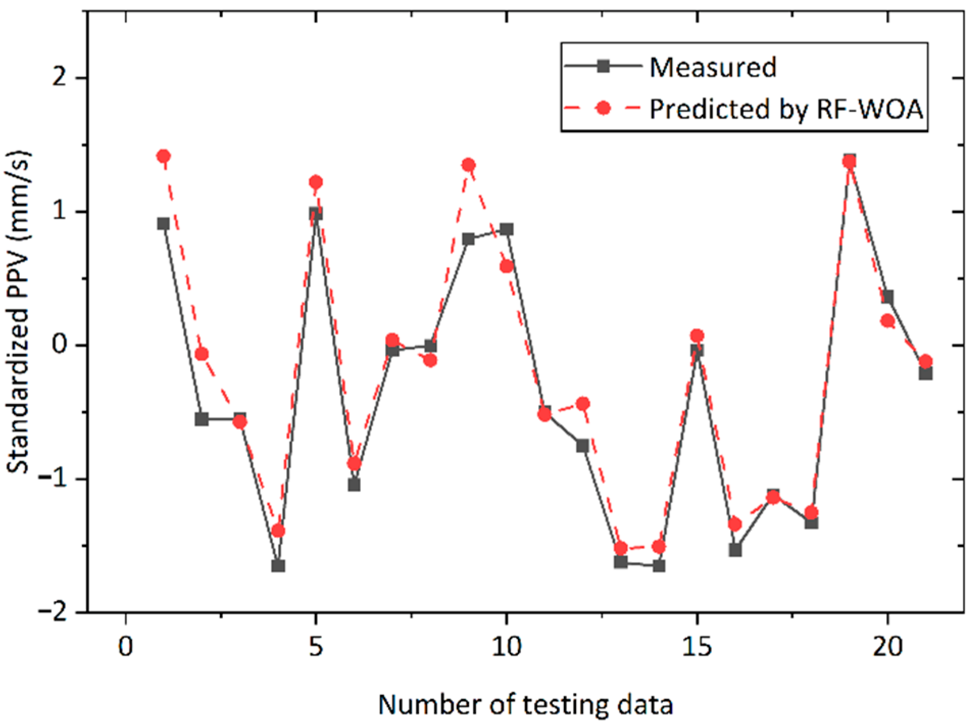
4.2. Improved RF-Based Models
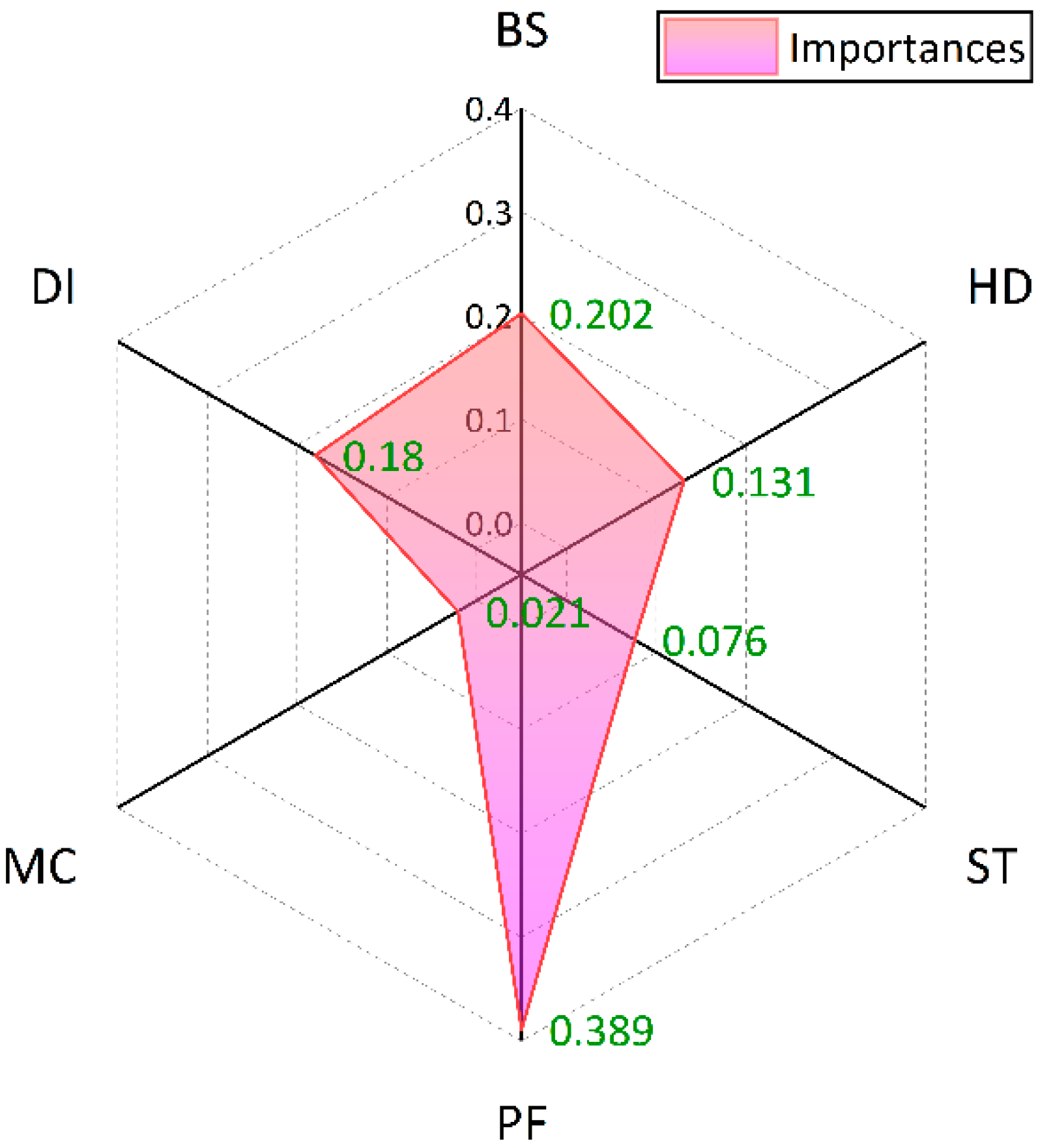
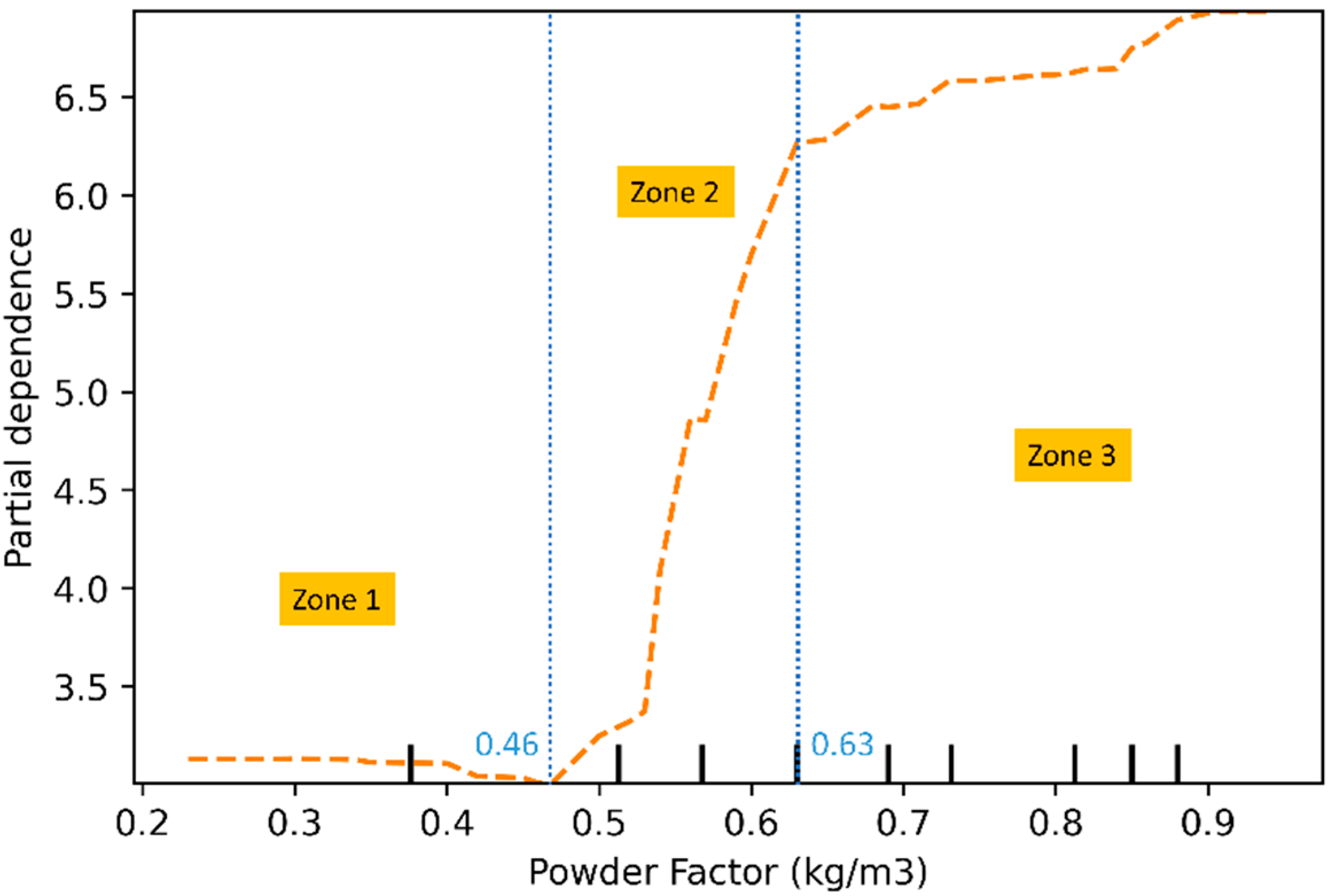
4.3. Sensitivity Analysis of Predictor Variables
4.4. Comparision with the Published Works
5. Conclusions
Author Contributions
Funding
Institutional Review Board Statement
Informed Consent Statement
Data Availability Statement
Acknowledgments
Conflicts of Interest
References
- Zhang, H.; Zhou, J.; Armaghani, D.J.; Tahir, M.M.; Pham, B.T.; Huynh, V. Van A Combination of Feature Selection and Random Forest Techniques to Solve a Problem Related to Blast-Induced Ground Vibration. Appl. Sci. 2020, 10, 869. [Google Scholar] [CrossRef] [Green Version]
- Hasanipanah, M.; Monjezi, M.; Shahnazar, A.; Armaghani, D.J.; Farazmand, A. Feasibility of indirect determination of blast induced ground vibration based on support vector machine. Measurement 2015, 75, 289–297. [Google Scholar] [CrossRef]
- Yu, Z.; Shi, X.; Zhou, J.; Gou, Y.; Huo, X.; Zhang, J.; Armaghani, D.J. A new multikernel relevance vector machine based on the HPSOGWO algorithm for predicting and controlling blast-induced ground vibration. Eng. Comput. 2020, 38, 905–1920. [Google Scholar] [CrossRef]
- Guo, H.; Zhou, J.; Koopialipoor, M.; Armaghani, D.J.; Tahir, M. Deep neural network and whale optimization algorithm to assess flyrock induced by blasting. Eng. Comput. 2021, 37, 173–186. [Google Scholar] [CrossRef]
- Zhou, J.; Koopialipoor, M.; Murlidhar, B.R.; Fatemi, S.A.; Tahir, M.M.; Armaghani, D.J.; Li, C. Use of intelligent methods to design effective pattern parameters of mine blasting to minimize flyrock distance. Nat. Resour. Res. 2020, 29, 625–639. [Google Scholar] [CrossRef]
- Guo, H.; Nguyen, H.; Bui, X.-N.; Armaghani, D.J. A new technique to predict fly-rock in bench blasting based on an ensemble of support vector regression and GLMNET. Eng. Comput. 2019, 37, 421–435. [Google Scholar] [CrossRef]
- Yu, Q.; Monjezi, M.; Mohammed, A.S.; Dehghani, H.; Armaghani, D.J.; Ulrikh, D.V. Optimized support vector machines combined with evolutionary random forest for prediction of back-break caused by blasting operation. Sustainability 2021, 13, 12797. [Google Scholar] [CrossRef]
- Sayadi, A.; Monjezi, M.; Talebi, N.; Khandelwal, M. A comparative study on the application of various artificial neural networks to simultaneous prediction of rock fragmentation and backbreak. J. Rock Mech. Geotech. Eng. 2013, 5, 318–324. [Google Scholar] [CrossRef] [Green Version]
- Faramarzi, F.; Farsangi, M.A.E.; Mansouri, H. An RES-based model for risk assessment and prediction of backbreak in bench blasting. Rock Mech. Rock Eng. 2013, 46, 877–887. [Google Scholar] [CrossRef]
- Afeni, T.B.; Osasan, S.K. Assessment of noise and ground vibration induced during blasting operations in an open pit mine—A case study on Ewekoro limestone quarry, Nigeria. Min. Sci. Technol. 2009, 19, 420–424. [Google Scholar] [CrossRef]
- He, B.; Armaghani, D.J.; Lai, S.H. A Short Overview of Soft Computing Techniques in Tunnel Construction. Open Constr. Build. Technol. J. 2022, 16, 1–6. [Google Scholar] [CrossRef]
- Lawal, A.I.; Kwon, S.; Kim, G.Y. Prediction of the blast-induced ground vibration in tunnel blasting using ANN, moth-flame optimized ANN, and gene expression programming. Acta Geophys. 2021, 69, 161–174. [Google Scholar] [CrossRef]
- Rai, R.; Shrivastva, B.K.; Singh, T.N. Prediction of maximum safe charge per delay in surface mining. Trans. Inst. Min. Metall. Sect. A Min. Technol. 2005, 114, 227–232. [Google Scholar] [CrossRef]
- Hasanipanah, M.; Bakhshandeh Amnieh, H.; Khamesi, H.; Jahed Armaghani, D.; Bagheri Golzar, S.; Shahnazar, A. Prediction of an environmental issue of mine blasting: An imperialistic competitive algorithm-based fuzzy system. Int. J. Environ. Sci. Technol. 2018, 15, 1–10. [Google Scholar] [CrossRef]
- Hasanipanah, M.; Faradonbeh, R.S.; Amnieh, H.B.; Armaghani, D.J.; Monjezi, M. Forecasting blast-induced ground vibration developing a CART model. Eng. Comput. 2017, 33, 307–316. [Google Scholar] [CrossRef]
- Ram Chandar, K.; Sastry, V.R.; Hegde, C.; Shreedharan, S. Prediction of peak particle velocity using multi regression analysis: Case studies. Geomech. Geoengin. 2017, 12, 207–214. [Google Scholar] [CrossRef]
- Khandelwal, M.; Singh, T.N. Prediction of blast induced ground vibrations and frequency in opencast mine: A neural network approach. J. Sound Vib. 2006, 289, 711–725. [Google Scholar] [CrossRef]
- Lawal, A.I.; Idris, M.A. An artificial neural network-based mathematical model for the prediction of blast-induced ground vibrations. Int. J. Environ. Stud. 2020, 77, 318–334. [Google Scholar] [CrossRef]
- Parida, A.; Mishra, M.K. Blast Vibration Analysis by Different Predictor Approaches—A Comparison. Procedia Earth Planet. Sci. 2015, 11, 337–345. [Google Scholar] [CrossRef] [Green Version]
- Xue, X.; Yang, X. Predicting blast-induced ground vibration using general regression neural network. JVC/J. Vib. Control 2014, 20, 1512–1519. [Google Scholar] [CrossRef]
- Yang, H.; Wang, Z.; Song, K. A new hybrid grey wolf optimizer-feature weighted-multiple kernel-support vector regression technique to predict TBM performance. Eng. Comput. 2020. [Google Scholar] [CrossRef]
- Yang, H.; Song, K.; Zhou, J. Automated Recognition Model of Geomechanical Information Based on Operational Data of Tunneling Boring Machines. Rock Mech. Rock Eng. 2022, 55, 1499–1516. [Google Scholar] [CrossRef]
- Armaghani, D.J.; Mohamad, E.T.; Narayanasamy, M.S.; Narita, N.; Yagiz, S. Development of hybrid intelligent models for predicting TBM penetration rate in hard rock condition. Tunn. Undergr. Sp. Technol. 2017, 63, 29–43. [Google Scholar] [CrossRef]
- Armaghani, D.J.; Koopialipoor, M.; Marto, A.; Yagiz, S. Application of several optimization techniques for estimating TBM advance rate in granitic rocks. J. Rock Mech. Geotech. Eng. 2019, 11, 779–789. [Google Scholar] [CrossRef]
- Zhou, J.; Yazdani Bejarbaneh, B.; Jahed Armaghani, D.; Tahir, M.M. Forecasting of TBM advance rate in hard rock condition based on artificial neural network and genetic programming techniques. Bull. Eng. Geol. Environ. 2020, 79, 2069–2084. [Google Scholar] [CrossRef]
- Li, Z.; Yazdani Bejarbaneh, B.; Asteris, P.G.; Koopialipoor, M.; Armaghani, D.J.; Tahir, M.M. A hybrid GEP and WOA approach to estimate the optimal penetration rate of TBM in granitic rock mass. Soft Comput. 2021, 25, 11877–11895. [Google Scholar] [CrossRef]
- Zhou, J.; Chen, C.; Wang, M.; Khandelwal, M. Proposing a novel comprehensive evaluation model for the coal burst liability in underground coal mines considering uncertainty factors. Int. J. Min. Sci. Technol. 2021, 31, 14. [Google Scholar] [CrossRef]
- Zhou, J.; Li, X.; Mitri, H.S. Classification of rockburst in underground projects: Comparison of ten supervised learning methods. J. Comput. Civ. Eng. 2016, 30, 4016003. [Google Scholar] [CrossRef]
- Pham, B.T.; Nguyen, M.D.; Nguyen-Thoi, T.; Ho, L.S.; Koopialipoor, M.; Kim Quoc, N.; Armaghani, D.J.; Le, H. Van A novel approach for classification of soils based on laboratory tests using Adaboost, Tree and ANN modeling. Transp. Geotech. 2021, 27, 100508. [Google Scholar] [CrossRef]
- Armaghani, D.J.; Harandizadeh, H.; Momeni, E.; Maizir, H.; Zhou, J. An Optimized System of GMDH-ANFIS Predictive Model by ICA for Estimating Pile Bearing Capacity; Springer: Cham, The Netherlands, 2022; Volume 55, ISBN 0123456789. [Google Scholar]
- Huat, C.Y.; Moosavi, S.M.H.; Mohammed, A.S.; Armaghani, D.J.; Ulrikh, D.V.; Monjezi, M.; Hin Lai, S. Factors Influencing Pile Friction Bearing Capacity: Proposing a Novel Procedure Based on Gradient Boosted Tree Technique. Sustainability 2021, 13, 11862. [Google Scholar] [CrossRef]
- Huang, J.; Sun, Y.; Zhang, J. Reduction of computational error by optimizing SVR kernel coefficients to simulate concrete compressive strength through the use of a human learning optimization algorithm. Eng. Comput. 2021. [Google Scholar] [CrossRef]
- Huang, J.; Kumar, G.S.; Ren, J.; Zhang, J.; Sun, Y. Accurately predicting dynamic modulus of asphalt mixtures in low-temperature regions using hybrid artificial intelligence model. Constr. Build. Mater. 2021, 297, 123655. [Google Scholar] [CrossRef]
- Asteris, P.G.; Lourenço, P.B.; Roussis, P.C.; Adami, C.E.; Armaghani, D.J.; Cavaleri, L.; Chalioris, C.E.; Hajihassani, M.; Lemonis, M.E.; Mohammed, A.S. Revealing the nature of metakaolin-based concrete materials using artificial intelligence techniques. Constr. Build. Mater. 2022, 322, 126500. [Google Scholar] [CrossRef]
- Mahmood, W.; Mohammed, A.S.; Asteris, P.G.; Kurda, R.; Armaghani, D.J. Modeling Flexural and Compressive Strengths Behaviour of Cement-Grouted Sands Modified with Water Reducer Polymer. Appl. Sci. 2022, 12, 1016. [Google Scholar] [CrossRef]
- Asteris, P.G.; Rizal, F.I.M.; Koopialipoor, M.; Roussis, P.C.; Ferentinou, M.; Armaghani, D.J.; Gordan, B. Slope Stability Classification under Seismic Conditions Using Several Tree-Based Intelligent Techniques. Appl. Sci. 2022, 12, 1753. [Google Scholar] [CrossRef]
- Cai, M.; Koopialipoor, M.; Armaghani, D.J.; Thai Pham, B. Evaluating Slope Deformation of Earth Dams due to Earthquake Shaking using MARS and GMDH Techniques. Appl. Sci. 2020, 10, 1486. [Google Scholar] [CrossRef] [Green Version]
- Zhou, J.; Dai, Y.; Khandelwal, M.; Monjezi, M.; Yu, Z.; Qiu, Y. Performance of Hybrid SCA-RF and HHO-RF Models for Predicting Backbreak in Open-Pit Mine Blasting Operations. Nat. Resour. Res. 2021, 30, 4753–4771. [Google Scholar] [CrossRef]
- Zhou, J.; Qiu, Y.; Khandelwal, M.; Zhu, S.; Zhang, X. Developing a hybrid model of Jaya algorithm-based extreme gradient boosting machine to estimate blast-induced ground vibrations. Int. J. Rock Mech. Min. Sci. 2021, 145, 104856. [Google Scholar] [CrossRef]
- Li, C.; Zhou, J.; Armaghani, D.J.; Li, X. Stability analysis of underground mine hard rock pillars via combination of finite difference methods, neural networks, and Monte Carlo simulation techniques. Undergr. Sp. 2021, 6, 379–395. [Google Scholar] [CrossRef]
- Parsajoo, M.; Armaghani, D.J.; Mohammed, A.S.; Khari, M.; Jahandari, S. Tensile strength prediction of rock material using non-destructive tests: A comparative intelligent study. Transp. Geotech. 2021, 31, 100652. [Google Scholar] [CrossRef]
- Asteris, P.G.; Mamou, A.; Hajihassani, M.; Hasanipanah, M.; Koopialipoor, M.; Le, T.-T.; Kardani, N.; Armaghani, D.J. Soft computing based closed form equations correlating L and N-type Schmidt hammer rebound numbers of rocks. Transp. Geotech. 2021, 29, 100588. [Google Scholar] [CrossRef]
- Momeni, E.; Armaghani, D.J.; Hajihassani, M.; Amin, M.F.M. Prediction of uniaxial compressive strength of rock samples using hybrid particle swarm optimization-based artificial neural networks. Measurement 2015, 60, 50–63. [Google Scholar] [CrossRef]
- Huang, J.; Zhang, J.; Gao, Y. Intelligently predict the rock joint shear strength using the support vector regression and Firefly Algorithm. Lithosphere 2021, 2021, 2467126. [Google Scholar] [CrossRef]
- Lawal, A.I. An artificial neural network-based mathematical model for the prediction of blast-induced ground vibration in granite quarries in Ibadan, Oyo State, Nigeria. Sci. African 2020, 8, e00413. [Google Scholar] [CrossRef]
- Rana, A.; Bhagat, N.K.; Jadaun, G.P.; Rukhaiyar, S.; Pain, A.; Singh, P.K. Predicting Blast-Induced Ground Vibrations in Some Indian Tunnels: A Comparison of Decision Tree, Artificial Neural Network and Multivariate Regression Methods. Min. Metall. Explor. 2020, 37, 1039–1053. [Google Scholar] [CrossRef]
- Lawal, A.I.; Kwon, S.; Hammed, O.S.; Idris, M.A. Blast-induced ground vibration prediction in granite quarries: An application of gene expression programming, ANFIS, and sine cosine algorithm optimized ANN. Int. J. Min. Sci. Technol. 2021, 31, 265–277. [Google Scholar] [CrossRef]
- Bui, X.N.; Nguyen, H.; Nguyen, T.A. Artificial Neural Network Optimized by Modified Particle Swarm Optimization for Predicting Peak Particle Velocity Induced by Blasting Operations in Open Pit Mines. Inz. Miner. 2021, 1, 79–90. [Google Scholar] [CrossRef]
- Iphar, M.; Yavuz, M.; Ak, H. Prediction of ground vibrations resulting from the blasting operations in an open-pit mine by adaptive neuro-fuzzy inference system. Environ. Geol. 2008, 56, 97–107. [Google Scholar] [CrossRef]
- Monjezi, M.; Ghafurikalajahi, M.; Bahrami, A. Prediction of blast-induced ground vibration using artificial neural networks. Tunn. Undergr. Sp. Technol. 2011, 26, 46–50. [Google Scholar] [CrossRef]
- Ghasemi, E.; Ataei, M.; Hashemolhosseini, H. Development of a fuzzy model for predicting ground vibration caused by rock blasting in surface mining. J. Vib. Control 2013, 19, 755–770. [Google Scholar] [CrossRef]
- Hajihassani, M.; Jahed Armaghani, D.; Marto, A.; Tonnizam Mohamad, E. Ground vibration prediction in quarry blasting through an artificial neural network optimized by imperialist competitive algorithm. Bull. Eng. Geol. Environ. 2014, 74, 873–886. [Google Scholar] [CrossRef]
- Armaghani, D.J.; Hasanipanah, M.; Amnieh, H.B.; Mohamad, E.T. Feasibility of ICA in approximating ground vibration resulting from mine blasting. Neural Comput. Appl. 2018, 29, 457–465. [Google Scholar] [CrossRef]
- Mohamed, M.T. Performance of fuzzy logic and artificial neural network in prediction of ground and air vibrations. Int. J. Rock Mech. Min. Sci. 2011, 39, 425–440. [Google Scholar]
- Breiman, L. Random Forests. Mach. Learn. 2001, 45, 5–32. [Google Scholar] [CrossRef] [Green Version]
- Mirjalili, S.; Mirjalili, S.M.; Lewis, A. Grey wolf optimizer. Adv. Eng. Softw. 2014, 69, 46–61. [Google Scholar] [CrossRef] [Green Version]
- Mirjalili, S.; Lewis, A. The whale optimization algorithm. Adv. Eng. Softw. 2016, 95, 51–67. [Google Scholar] [CrossRef]
- Kaur, S.; Awasthi, L.K.; Sangal, A.L.; Dhiman, G. Tunicate Swarm Algorithm: A new bio-inspired based metaheuristic paradigm for global optimization. Eng. Appl. Artif. Intell. 2020, 90, 103541. [Google Scholar] [CrossRef]
- Li, H.B.; Wang, W.; Ding, H.W.; Dong, J. Trees Weighting Random Forest method for classifying high-dimensional noisy data. In Proceedings of the 2010 IEEE 7th International Conference on E-Business Engineering, Shanghai, China, 10–12 November 2010; pp. 160–163. [Google Scholar]
- Zorlu, K.; Gokceoglu, C.; Ocakoglu, F.; Nefeslioglu, H.A.; Acikalin, S. Prediction of uniaxial compressive strength of sandstones using petrography-based models. Eng. Geol. 2008, 96, 141–158. [Google Scholar] [CrossRef]
- Taylor, K.E. Summarizing multiple aspects of model performance in a single diagram. J. Geophys. Res. Atmos. 2001, 106, 7183–7192. [Google Scholar] [CrossRef]
- Taylor, K.E. Taylor Diagram Primer—Working Paper. 2005. Available online: http://www.atmos.albany.edu/daes/atmclasses/atm401/spring_2016/ppts_pdfs/Taylor_diagram_primer.pdf (accessed on 10 May 2022).
- Friedman, J.H. Greedy function approximation: A gradient boosting machine. Ann. Stat. 2001, 29, 1189–1232. [Google Scholar] [CrossRef]
- Shirani Faradonbeh, R.; Jahed Armaghani, D.; Abd Majid, M.Z.; MD Tahir, M.; Ramesh Murlidhar, B.; Monjezi, M.; Wong, H.M. Prediction of ground vibration due to quarry blasting based on gene expression programming: A new model for peak particle velocity prediction. Int. J. Environ. Sci. Technol. 2016, 13, 1453–1464. [Google Scholar] [CrossRef] [Green Version]
- Zhou, J.; Asteris, P.G.; Armaghani, D.J.; Pham, B.T. Prediction of ground vibration induced by blasting operations through the use of the Bayesian Network and random forest models. Soil Dyn. Earthq. Eng. 2020, 139, 106390. [Google Scholar] [CrossRef]


| Techniques | Input Variables | Number of Samples | Studies |
|---|---|---|---|
| RF, CART, CHAID, SVM, ANN | MC, HD, ST, PF, DI | 102 | Zhang et al. [1] |
| ANN | DI, MC | 100 | Lawal, A.I. [45] |
| GEP, ANFIS, SCA-ANN | DI, MC, ρ, SRH | 100 | Lawal, A.I. et al. [47] |
| MPSO-ANN | DI, MC | 137 | BUI Xuan-Nam et al. [48] |
| ANN, DT | TC, A, MC, NH, H, DI, HD, CPH | 137 | Rana et al. [46] |
| ANFIS | DI, MC | 44 | Iphar et al. [49] |
| ANN | HD, ST, DI, MC | 182 | Monjezi et al. [50] |
| FIS | B, S, ST, N, MC, DI | 120 | Ghasemi et al. [51] |
| ICA-ANN | BS, ST, MC, DI, Vp, E | 95 | Hajmassani et al. [52] |
| ICA | MC, DI | 73 | Jahed Armaghani et al. [53] |
| ANN, FIS | MC, DI | 162 | Mohamed [54] |
| Parameters | Symbol | Unit | Type | Max | Min | Mean | Std. Dev. |
|---|---|---|---|---|---|---|---|
| Burden to spacing | BS | - | Input | 0.92 | 0.7 | 0.819 | 0.004 |
| Hole depth | HD | m | Input | 23.17 | 5.23 | 14.115 | 15.973 |
| Stemming | ST | m | Input | 3.6 | 1.9 | 2.630 | 0.157 |
| Powder factor | PF | kg/m3 | Input | 0.94 | 0.23 | 0.654 | 0.034 |
| Max charge per delay | MC | kg | Input | 305.6 | 45.8 | 179.623 | 4246.587 |
| Distance | DI | m | Input | 531 | 285 | 379.520 | 5100.269 |
| Peak particle velocity | PPV | mm/s | Output | 11.05 | 0.13 | 5.337 | 9.267 |
| Models | Training | Testing | Score Summation | |||||||||||||||
|---|---|---|---|---|---|---|---|---|---|---|---|---|---|---|---|---|---|---|
| Swarm Size | R2 | Score | RMSE | Score | MAE | Score | VAF | Score | R2 | Score | RMSE | Score | MAE | Score | VAF | Score | ||
| RF-WOA | 50 | 0.986 | 4 | 0.119 | 1 | 0.094 | 2 | 98.584 | 1 | 0.932 | 4 | 0.246 | 4 | 0.187 | 4 | 94.723 | 3 | 23 |
| 100 | 0.986 | 4 | 0.118 | 2 | 0.093 | 3 | 98.603 | 2 | 0.932 | 4 | 0.246 | 4 | 0.188 | 3 | 95.032 | 4 | 26 | |
| 150 | 0.986 | 4 | 0.117 | 3 | 0.092 | 4 | 98.612 | 3 | 0.927 | 2 | 0.254 | 2 | 0.191 | 2 | 94.430 | 2 | 22 | |
| 200 | 0.986 | 4 | 0.116 | 4 | 0.092 | 4 | 98.647 | 4 | 0.928 | 3 | 0.253 | 3 | 0.196 | 1 | 94.394 | 1 | 24 | |
| Models | Training | Testing | Score Summation | |||||||||||||||
|---|---|---|---|---|---|---|---|---|---|---|---|---|---|---|---|---|---|---|
| Swarm Size | R2 | Score | RMSE | Score | MAE | Score | VAF | Score | R2 | Score | RMSE | Score | MAE | Score | VAF | Score | ||
| RF-GWO | 50 | 0.986 | 4 | 0.116 | 4 | 0.092 | 4 | 98.632 | 1 | 0.930 | 4 | 0.250 | 4 | 0.192 | 3 | 94.516 | 3 | 27 |
| 100 | 0.986 | 4 | 0.116 | 4 | 0.092 | 4 | 98.633 | 2 | 0.929 | 3 | 0.251 | 3 | 0.192 | 3 | 94.475 | 1 | 24 | |
| 150 | 0.986 | 4 | 0.116 | 4 | 0.092 | 4 | 98.637 | 4 | 0.929 | 3 | 0.252 | 2 | 0.193 | 2 | 94.488 | 2 | 25 | |
| 200 | 0.986 | 4 | 0.116 | 4 | 0.093 | 3 | 98.635 | 3 | 0.929 | 3 | 0.251 | 3 | 0.191 | 4 | 94.528 | 4 | 28 | |
| Models | Training | Testing | Score Summation | |||||||||||||||
|---|---|---|---|---|---|---|---|---|---|---|---|---|---|---|---|---|---|---|
| Swarm Size | R2 | Score | RMSE | Score | MAE | Score | VAF | Score | R2 | Score | RMSE | Score | MAE | Score | VAF | Score | ||
| RF-TSA | 50 | 0.986 | 4 | 0.118 | 2 | 0.093 | 3 | 98.598 | 2 | 0.931 | 4 | 0.248 | 4 | 0.191 | 4 | 94.743 | 4 | 27 |
| 100 | 0.986 | 4 | 0.118 | 2 | 0.094 | 2 | 98.582 | 1 | 0.924 | 1 | 0.260 | 1 | 0.201 | 2 | 93.823 | 1 | 14 | |
| 150 | 0.986 | 4 | 0.116 | 4 | 0.093 | 3 | 98.635 | 4 | 0.927 | 2 | 0.255 | 2 | 0.191 | 4 | 94.483 | 2 | 25 | |
| 200 | 0.986 | 4 | 0.117 | 3 | 0.092 | 4 | 98.619 | 3 | 0.929 | 3 | 0.251 | 3 | 0.195 | 3 | 94.569 | 3 | 26 | |
| Models | Training | Testing | Score Summation | ||||||||||||||
|---|---|---|---|---|---|---|---|---|---|---|---|---|---|---|---|---|---|
| R2 | Score | RMSE | Score | MAE | Score | VAF | Score | R2 | Score | RMSE | Score | MAE | Score | VAF | Score | ||
| RF-WOA (100) | 0.986 | 6 | 0.118 | 5 | 0.093 | 6 | 98.603 | 5 | 0.932 | 6 | 0.246 | 6 | 0.188 | 6 | 95.032 | 6 | 46 |
| RF-GWO (200) | 0.986 | 6 | 0.116 | 6 | 0.093 | 6 | 98.635 | 6 | 0.929 | 4 | 0.251 | 4 | 0.191 | 5 | 94.528 | 4 | 41 |
| RF-TSA (50) | 0.986 | 6 | 0.118 | 5 | 0.093 | 6 | 98.598 | 4 | 0.931 | 5 | 0.248 | 5 | 0.191 | 5 | 94.743 | 5 | 41 |
| RF | 0.973 | 3 | 0.164 | 2 | 0.123 | 3 | 97.298 | 1 | 0.923 | 1 | 0.262 | 1 | 0.209 | 2 | 93.994 | 1 | 14 |
| RF-R2 | 0.974 | 4 | 0.161 | 3 | 0.121 | 4 | 97.380 | 2 | 0.924 | 2 | 0.261 | 2 | 0.207 | 3 | 94.078 | 2 | 22 |
| RF-RMSE | 0.975 | 5 | 0.156 | 4 | 0.119 | 5 | 97.530 | 3 | 0.925 | 3 | 0.258 | 3 | 0.203 | 4 | 94.219 | 3 | 30 |
| Reference | Models | Training | Testing | ||||||
|---|---|---|---|---|---|---|---|---|---|
| R2 | RMSE | MAE | VAF | R2 | RMSE | MAE | VAF | ||
| Present paper | RF-WOA | 0.986 | 0.118 | 0.093 | 98.603 | 0.932 | 0.246 | 0.188 | 95.032 |
| [64] | GEP | 0.914 | 0.920 | 0.755 | 91.304 | 0.874 | 0.963 | 0.851 | 87.107 |
| NLMR | 0.829 | 1.365 | 1.125 | 80.878 | 0.790 | 1.498 | 1.221 | 69.261 | |
| [1] | RF | 0.940 | 0.770 | 0.620 | 92.970 | 0.830 | 1.460 | 1.190 | 82.170 |
| CART | 0.670 | 1.670 | 1.320 | 67.030 | 0.560 | 2.390 | 1.840 | 54.600 | |
| CHAID | 0.910 | 0.860 | 0.540 | 91.300 | 0.680 | 1.900 | 1.470 | 67.790 | |
| ANN | 0.890 | 0.960 | 0.750 | 89.140 | 0.840 | 1.410 | 1.130 | 83.710 | |
| SVM | 0.880 | 1.020 | 0.770 | 88.480 | 0.850 | 1.500 | 1.170 | 84.540 | |
| [65] | RF | 0.930 | - | - | - | 0.903 | - | - | - |
| BN | 0.930 | - | - | - | 0.871 | - | - | - | |
Publisher’s Note: MDPI stays neutral with regard to jurisdictional claims in published maps and institutional affiliations. |
© 2022 by the authors. Licensee MDPI, Basel, Switzerland. This article is an open access article distributed under the terms and conditions of the Creative Commons Attribution (CC BY) license (https://creativecommons.org/licenses/by/4.0/).
Share and Cite
He, B.; Lai, S.H.; Mohammed, A.S.; Sabri, M.M.S.; Ulrikh, D.V. Estimation of Blast-Induced Peak Particle Velocity through the Improved Weighted Random Forest Technique. Appl. Sci. 2022, 12, 5019. https://doi.org/10.3390/app12105019
He B, Lai SH, Mohammed AS, Sabri MMS, Ulrikh DV. Estimation of Blast-Induced Peak Particle Velocity through the Improved Weighted Random Forest Technique. Applied Sciences. 2022; 12(10):5019. https://doi.org/10.3390/app12105019
Chicago/Turabian StyleHe, Biao, Sai Hin Lai, Ahmed Salih Mohammed, Mohanad Muayad Sabri Sabri, and Dmitrii Vladimirovich Ulrikh. 2022. "Estimation of Blast-Induced Peak Particle Velocity through the Improved Weighted Random Forest Technique" Applied Sciences 12, no. 10: 5019. https://doi.org/10.3390/app12105019
APA StyleHe, B., Lai, S. H., Mohammed, A. S., Sabri, M. M. S., & Ulrikh, D. V. (2022). Estimation of Blast-Induced Peak Particle Velocity through the Improved Weighted Random Forest Technique. Applied Sciences, 12(10), 5019. https://doi.org/10.3390/app12105019