Abstract
Rolled carbon steel sheets used in industrial and construction sites are formed by passing metal stock between two rotating rolls using a rolling mill, and the work roll is an essential part of the rolling mill. As the work rolls are in direct contact with the workpiece, the process quality is highly sensitive to their surface integrity, which is maintained through rough and finish cuttings; ultrasonic inspection is often performed after rough cutting the surfaces of work rolls. Ultrasonic inspection signals comprise signals reflected from and below the surface. Depending on the size of the subsurface defects, the thickness of the finish cutting is determined. The signals reflected by defects close to the surface overlap with those from the work roll surface, which is referred to as the ultrasonic dead zone and makes defect detection difficult. Since visual detection of flaws is not possible from signals collected from the dead zone, finish cutting is commonly performed up to the dead zone depth; this requires unnecessary cost and process time, which must be improved. Therefore, in this study a convolutional neural network is used to improve defect detection performance in the ultrasonic dead zone during the inspection of work rolls.
1. Introduction
Large-scale cold rolling processes generally use a 6-high tandem rolling mill consisting of work rolls, intermediate rolls, and backup rolls. The rolling mill used in the process feeds high-temperature or room-temperature metal stock between two rotating rolls to form materials in various shapes. Among the components, the work roll is a core part of the rolling mill; since the work roll is in direct contact with the workpiece to produce cold rolled carbon sheets of the required thickness, it must have very high strength and hardness. In particular, if there are micro-defects near the surface of the work roll, they may cause damage to the rolled product. Therefore, meticulous monitoring and control of the surface of the work roll to a certain depth are required, and ultrasonic inspection is used for this purpose. Currently, work rolls are roughly cut prior to conducting ultrasonic inspection, and based on the results of the inspection, finish cutting is performed. However, a dead zone for the inspection signals is seen in ultrasonic inspection owing to the initial ultrasonic signals, and if the defect signals overlap in the dead zone, it is difficult to identify defects. Therefore, finish cutting of the work rolls is performed based on the flaws detected in the region beyond the dead zone. However, this may incur unnecessary processing time and cost, which may result in significant losses to the manufacturer. Hence, detecting defects in the ultrasonic dead zone is instrumental in the industrial process [1,2,3].
To reduce the ultrasonic dead zone, one of the methods employed is to minimize the initial pulse of the ultrasonic waves by adjusting the band width, and another method is to shift the ultrasonic frequency to a higher frequency to reduce ultrasonic ringing. Further, there is a method of minimizing the initial pulse using a dual ultrasonic probe, and another method of removing the initial pulse effects by introducing a gap between the specimen and ultrasonic probe using an immersion transducer. However, even with the immersion transducer, the ultrasonic dead zone is formed near the surface by the reflected signals generated at the interface between the water and the specimen. Therefore, although the size of the dead zone can be reduced by adjusting different variables, such as the general method of ultrasonic inspection and the transducer, it is difficult to fundamentally remove the dead zone [4,5,6].
Therefore, most studies on work rolls mainly investigate methods to increase the hardness and strength of the work roll itself rather than ultrasonic inspection techniques. Lim et al. studied the forging process using ultrahigh carbon steel for the work roll [7], and Park et al. developed the N_HSR1 with improved wear resistance and roll failure in response to the changing rolling conditions [8]. Garza-Montes-de-Oca et al. investigated degradation mechanisms for abrasive wear and thermal fatigue on the surface of the work roll [9]. In addition, Li et al. investigated the surface temperature field of the work rolls using finite element method (FEM) simulations based on the thermal conduction equation and analyzed the work roll surface temperature, thermal stress, and thermal fatigue [10]. Benasciutti et al. used the FEM to investigate a simplified numerical approach for calculating heat by the rotation acting on the surface of the work roll and load generated in the cooling process [11]. Among these previous studies, a few were based on ultrasonic inspection of the work rolls, and it is seen that further research is needed on methods to reduce the problems of cost and time in the manufacturing process of the work rolls. Therefore, the signals from the dead zone, which are difficult to detect by human judgment based on visual observations, are acquired in this study through a standard specimen, and a convolutional neural network (CNN), which is one of the types of deep-learning network, is used to determine the status of defects in the dead zone and classify them.
2. Experimental Procedures
2.1. Specimen
In current practice, ultrasonic inspection of work rolls is performed by applying the local water immersion method using a resolution-type immersion transducer (Olympus, Seoul, Korea, 10 MHz, 0.25″). Figure 1 shows the typical ultrasonic inspection system for work rolls employed in industrial sites.
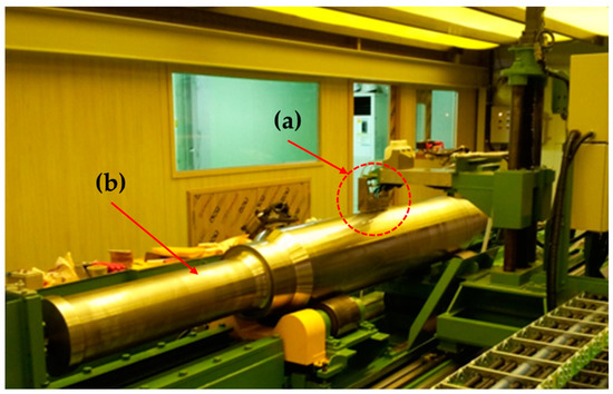
Figure 1.
Ultrasonic inspection system for work rolls: (a) sensor module and (b) work roll.
In the actual site, the minimum defect size that can be detected by ultrasonic inspection of the work rolls is 0.4 mm, and the ultrasonic signals are amplified to detect the micro-defects. As the gain of the ultrasonic pulser receiver increases, the signals from the work roll surface generated at the interface between the water and the work roll overlap with the defect signal generated immediately below the surface. Figure 2 presents a schematic illustration of the inspection of a work roll.
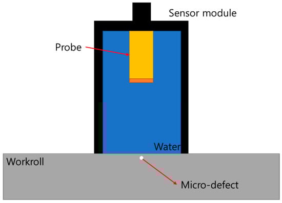
Figure 2.
Schematic of ultrasonic inspection of the work roll.
In this study, to improve the problem caused by the dead zone in the ultrasonic inspection of work rolls using deep learning, a standard specimen modeling the subsurface defects in the work roll was fabricated. The standard specimen was made of AISI 304L, a material similar to that of the work roll, with defects of size 0.4 mm; the defects are of the side drilled hole (SDH) type and are located at depths 1 mm, 2 mm, 3 mm, and 4 mm below the surface. The spacing between the defects is set as 20 mm so as not to affect the ultrasonic signals. Figure 3 shows the fabricated standard specimen.
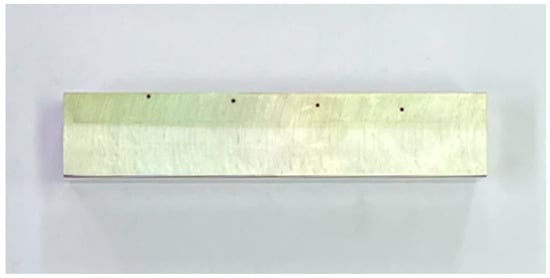
Figure 3.
Fabricated standard specimen.
2.2. Experimental Setup
The signals from the subsurface defects were acquired using the standard specimen, and the sensor module of the ultrasonic inspection system for the work rolls was modeled with an ultrasonic C-scanner, as shown in Figure 4. Figure 4 shows a photograph of the ultrasonic C-scanner used in the experiments.
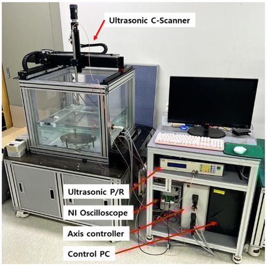
Figure 4.
Ultrasonic C-scanner used in this study.
The transducer used in the experiment was a water-immersion-type device (Olympus, 10 MHz, 0.25″) that is used in actual industrial sites. Moreover, the gain of the ultrasonic pulser receiver was adjusted to detect and differentiate the defect signals. Figure 5 shows the ultrasonic A-scan signals of the defects in the standard specimen for the respective cases. Figure 5a shows signals with no defects, and Figure 5b–e shows the signals of the defects at depths of 1 mm, 2 mm, 3 mm, and 4 mm below the surface, respectively. In Figure 5d,e, the signals reflected from the surface and those from the subsurface defects are observed to overlap, which actually shows similar signal patterns to those in Figure 5a without the defects. This indicates that in such cases it is difficult to determine the presence or absence of defects by intuitive human judgment based on visual observations.
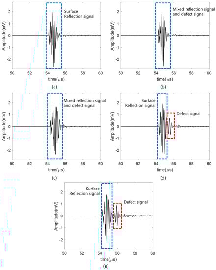
Figure 5.
Ultrasonic A−scan signals of the standard specimen: (a) without defects; with defects below the surface at depths of (b) 1 mm, (c) 2 mm, (d) 3 mm, and (e) 4 mm.
3. Database Implementation
3.1. Ultrasonic Database
To train the CNN, a database was developed from the collected ultrasonic signals, as shown in Figure 5, and the database specifications are as shown in Table 1.

Table 1.
Ultrasonic defect database.
In the case of signals without defects, 700 sets of data were collected, and 350 signals each were collected for defects at depths of 1 mm and 2 mm below the surface. In addition, to test the performance of the trained neural network, 20% of the collected signals were randomly selected; the training database was constructed with 1200 signals, and the test database was separately constructed with 200 signals.
3.2. Database Augmentation
A total of 1400 ultrasonic signals were collected, including the training and test data, but this amount of data is insufficient considering the reliability of deep-learning results. Therefore, the database was augmented using two methods [12,13,14], and the effectiveness of these two methods has been verified in the previous studies. First, white Gaussian noise (WGN) with a signal-to-noise ratio (SNR) was added to the existing signals for data augmentation. Because the ultrasonic inspections are generally performed in harsh environments, the signals are highly sensitive to noise; in particular, since the inspection results may be compromised by electrical noise that occurs as WGN, the data was increased by adding WGN with SNR. Hence, based on the number of existing data, the total amount of data increased sixfold from 1400 to 8400.
Second, the data were augmented by simulating the time-axis shifting of the ultrasonic signals. For ultrasonic signals, the time axis of the defect reflection signals may shift owing to the influence of the experimental settings and equipment. Based on the existing signal data, the number of data was increased by shifting the time axis by 0.5–1.5 μs, and the total number of data increased sixfold from 1400 to 8400. Figure 6 shows the ultrasonic signals of the augmented data, and Table 2 shows the composition of the augmented database based on the original database.
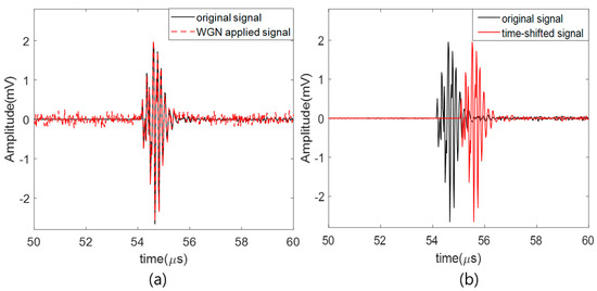
Figure 6.
Augmented ultrasonic signal: (a) applied WGN with SNR, (b) time shifting.
Table 2.
Augmented database.
4. Artificial Neural Networks
Artificial neural networks (ANN) refer to statistical learning algorithms used in machine learning and cognitive sciences inspired by neural networks in biology. The first ANN was proposed by McCulloch and Pitts [15]; then, Rosenblatt [16,17] developed the perceptron, which is an ANN for supervised self-learning; the essence of training the neural network is the backpropagation algorithm, which was proposed by Werbos [18] and Rumelhart [19].
The ANN consists of an input layer, a hidden layer, and an output layer. Each layer contains nodes assigned with weights and is a feed-forward network with the inputs processed only in the forward direction to all nodes in the next layer. In the learning process of a neural network, the external data are first received from the input layer, features of the data are extracted from the hidden layer, and the output layer produces a result derived from the extracted features and presents this result as an output. In most cases, neural network models have one each of the input and output layers, but the number of hidden layers can vary depending on the complexity of the problem. The case with more than one hidden layer is referred to as a deep neural network (DNN). Given the same data output from the previous layer, different features are extracted for each neuron from the same input data, and the output is calculated using weighted summation and activation functions during feature extraction. After calculating the output, the error between the real data and the predicted output is provided using a loss function, and the backpropagation algorithm is used to reduce the error as well as fine-tune the weights again [17,20,21,22].
4.1. CNN
The CNN is a class of ANN proposed by Le Cun et al. [23] and follows the design concept and model architecture of the neocognitron [24] while adopting the backpropagation algorithm for learning; it is currently the most commonly applied ANN. The CNN can be divided into one part for extracting the features of the input data and another part for classifying these features. The feature extraction part is divided into the convolutional and pooling layers. In the convolutional layer, the main operation is a convolution, and the pooling layer provides spatial transformation invariance via a pooling operation. The convolutional and pooling layers correspond to the simple and complex cell layers of the neocognitron, respectively, and the convolutional layer is an essential element for introducing an activation function after applying a filter to the input data. The pooling layer of the neural network performs subsampling of the input data to reduce the computational load and prevent overfitting; however, as it increases the complexity, its use can be selected depending on the problem. For classification, a flatten layer is located in the middle, through which the data are transformed into an array connection to a fully connected layer. With the CNN, a pattern can be learned in one location and determined in another location, which is possible by sharing the same parameters in the filter [13,25,26,27]. Figure 7 shows the architecture of the CNN described above.
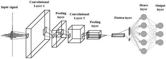
Figure 7.
Architecture of the convolutional neural network.
4.2. Architecture of the CNN
In this study, a CNN designed with Keras based on TensorFlow (Google “open-source software for deep learning”) was used, which consists of an input layer, three convolutional layers, three pooling layers, a fully connected layer, and an output layer. The number of nodes in the input layer is 2500, which is the same as the number of sampling points in the signals. Table 3 outlines the parameters used in the CNN.
Table 3.
Parameters of the CNN.
The filter size of the first convolutional layer was set to 1 × 16 to achieve good performance even in conditions with excess noise in the signals [13]; to prevent overfitting during training, a dropout layer was added after each convolutional layer. In addition, to reduce the computational load and prevent overfitting, a pooling layer was added after the dropout layer, and the kernel size (1 × 2) and stride (1 × 2) were set. The filter sizes of the second and third convolutional layers were reduced to 1 × 8 each, and a dropout and pooling layers were added, respectively. The dropout parameter was set to 0.5. The number of nodes of the fully connected layer was set to 300, and the number of nodes that provided good performance was selected through multiple trials.
For the output layers, since there are three types of signals, namely signals without defects and defect signals from depths 1 mm and 2 mm below the surface, the number was set to 3. For the activation function used in the convolution layer, the ReLU function was used, which showed good performance for deep learning [13,27,28,29,30]; the sigmoid function was not used because the output value of the function converges to 0 when there are many layers [13,25]. The ReLU function is expressed as Equation (1) below.
In addition, sparse categorical cross-entropy was used as the loss function and is expressed as Equation (2).
where D is the number of data, y is a vector of the true labels, and p is the vector of predicted labels. Sparse categorical cross-entropy provides results in integer form and is widely used for multiclass classifications. For the output layer activation function, softmax is used and is expressed as Equation (3) below:
where y is the input vector to the output layer, and i indexes the output nodes, i = 1, 2, …, k. In this study, the number of classes is 3, so k = 3.
4.3. Performance Evaluation of the CNN
The performance of the proposed CNN was evaluated using the augmented database in Table 2. Figure 8 shows the performance of the CNN for 500 epochs. The black line in Figure 8 represents the training accuracy, and it can be seen to start with an accuracy of 50.8%, to rapidly increase to 95.8% until 50 epochs, and to further increase to 99% at 250 epochs, thus confirming that the training reaches saturation. The red line indicates the test accuracy, which starts at 58.58% in the first epoch, increases rapidly to 94.04% until 90 epochs, and reaches saturation at about 280 epochs with a gradual increase to 98.54%. Subsequently, at about 225 epochs, there is no further improvement in the performance. When the epoch number was 90 ≤ epoch ≤ 300, the accuracy was 95.58% ± 1.28%, and when the epoch number was 300 < epoch ≤ 500, the accuracy was 98.57% ± 0.66%. If 90 epochs are considered as the saturation point, then the accuracy is 97.19% ± 1.8%. Figure 9 illustrates the evaluation of the defect classification accuracy of the proposed CNN.

Figure 8.
CNN training performance with the augmented database.
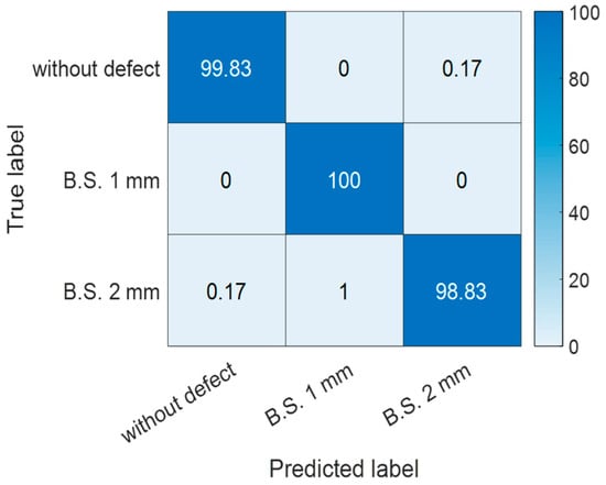
Figure 9.
Defect classification accuracy of the CNN (B.S.: below surface).
The probability of accurately classifying a signal without defects was 99.83%, and the probability of incorrect classification as defect at 2 mm below the surface was 0.17%. Correct classification was performed for defects that were 1 mm below the surface; the probability of incorrect classification of the defects at 2 mm below the surface as defects at 1 mm below the surface was 1%, and the probably of correct classification of the defects at 2 mm below the surface was 98.83%. In most cases, it is confirmed that the prediction performance for defect classification was almost accurate.
5. Conclusions
A rolling mill is an equipment used to produce cold-rolled carbon steel sheets, and its main component is the work roll. Because the work roll affects the product quality of the cold-rolled carbon sheets based on its surface integrity, quality control is performed with strict standards; to this end, ultrasonic inspections are often performed. In this study, we investigated a method for improving the detectability in the dead zone for ultrasonic inspection performed to evaluate the integrity of the work rolls.
First, a standard specimen model of a work roll with defects was fabricated, and defect signals were collected according to signal type using an ultrasonic C-scanner as in the real ultrasonic inspection system for work rolls. In the collected ultrasonic signals, overlaps were observed between the ultrasonic signals reflected from the work roll surface and subsurface defect signals. In the case without defects, signal patterns for the defects 1 mm and 2 mm below the surface were similar, rendering differentiation by visual observation difficult. However, for defects 3 mm and 4 mm below the surface, differentiation by visual observation was possible. For signals that could not be differentiated by visual inspection, about 1400 signals were acquired, and the database was expanded by data augmentation. Then, deep learning was performed using a CNN. Through the process of training and testing, it was confirmed that the CNN could achieve an accuracy of about 97.19% ± 1.8%. In future research, it is expected that practical industrial site-oriented investigations may be required to overcome the difficulties arising with the use of the developed CNN when applied to data at real industrial sites.
Author Contributions
Conceptualization, H.-J.K. and H.-H.K.; methodology, H.-J.K. and Y.-T.Y.; software, H.-J.K.; validation, H.-J.K., H.-H.K., and S.-J.S.; formal analysis, H.-H.K. and J.P.; investigation, H.-H.K.; resources, H.-J.K.; data curation, Y.-T.Y., H.-H.K., and J.P.; writing—original draft preparation, Y.-T.Y. and H.-H.K.; writing—review and editing, H.-J.K. and S.-J.S.; visualization, H.-J.K.; supervision, H.-H.K. and S.-J.S.; project administration, H.-J.K.; funding acquisition, H.-J.K. All authors have read and agreed to the published version of the manuscript.
Funding
This work has supported by the National Research Foundation of Korea (NRF) grant funded by the Korea government (MSIT) (No. NRF-2020R1I1A1A01070133).
Institutional Review Board Statement
Not applicable.
Informed Consent Statement
Not applicable.
Data Availability Statement
The data that support the findings of this study are available from the corresponding author upon reasonable request.
Conflicts of Interest
The authors declare no conflict of interest.
References
- Sinha, P.; Indimath, S.S.; Mukhopadhyay, G.; Bhattacharyya, S. Failure of a work roll of a thin strip rolling mill: A case study. Procedia Eng. 2014, 86, 940–948. [Google Scholar] [CrossRef]
- Carretta, Y.; Hunter, A.K.; Boman, R.; Ponthot, J.-P.; Legrand, N.; Laugier, M.; Dwyer-Joyce, R.S. Ultrasonic roll bite measurements in cold rolling-roll stress and deformation. J. Mater. Process. Technol. 2017, 249, 1–13. [Google Scholar] [CrossRef]
- Singh, K.; Mondal, N.; Mandal, C.; Prasad, R.; Sengupta, P. Application of ultrasonic and eddy current testing for inspection of rolls. NDTnet 2014, 2, 1–9. [Google Scholar]
- Salim, M.; Malek, M.; Sabri, N.; Juni, K. Study on ringing effect in ultrasonic transducer. Sci. Res. Essays 2012, 43, 3682–3689. [Google Scholar]
- Schmerr, L. Fundamentals of Ultrasonic Nondestructive Evaluation: A Modeling Approach, 1st ed.; Plenum Press: New York, NY, USA, 1998; pp. 91–140. ISBN 0-306-45752-0. [Google Scholar]
- Schmerr, L.; Song, S. Ultrasonic Nondestructive Evaluation Systems: Models and Measurements, 1st ed.; Springer: New York, NY, USA, 2010; pp. 127–231. ISBN 978-0-387-49061-8. [Google Scholar]
- Lim, H.; Lee, H.; Kim, B.; Kang, S. Process design for manufacturing 1.5 wt%C ultrahigh carbon workroll: Void closure behavior and bonding strength. Trans. Mater. Process. 2013, 22, 269–274. [Google Scholar] [CrossRef]
- Park, S.; Lee, J.; Weon, J.; Lee, W.; Yoon, J.; Park, Y. An improved alloy for forged rolls for cold rolling. Kor. Soc. Technol. Plas. Roll. Symp. 2009, 65–71. [Google Scholar]
- Garza-Montes-de-Oca, N.; Rainforth, W. Wear mechanisms experienced by a work roll grade high speed steel under different environmental conditions. Wear 2009, 267, 441–448. [Google Scholar] [CrossRef]
- Li, C.; Yu, H.; Deng, G.; Liu, X.; Wang, G. Numerical simulation of temperature field and thermal stress field of work roll during hot strip rolling. J. Iron Steel Res. 2007, 14, 18–21. [Google Scholar] [CrossRef]
- Benasciuttia, D.; Brusab, E.; Bazzaro, G. Finite elements prediction of thermal stresses in work roll of hot rolling mills. Procedia Eng. 2010, 2, 707–716. [Google Scholar] [CrossRef]
- Polikar, R.; Udpa, L.; Udpa, S.S.; Taylor, T. Frequency invariant classification of ultrasonic weld inspection signals. IEEE Trans. Ultrason. Ferroelectr. Freq. Control 1998, 45, 614–625. [Google Scholar] [CrossRef] [PubMed]
- Munir, N.; Kim, H.J.; Park, J.; Song, S.J.; Kang, S.S. Convolutional neural network for ultrasonic weldment flaw classification in noisy conditions. Ultrasonics 2019, 94, 74–81. [Google Scholar] [CrossRef] [PubMed]
- Rimoldi, B. Principles of Digital Communication: A Top-Down Approach; Cambridge University Press: Cambridge, UK, 2016. [Google Scholar]
- McCulloch, W.; Pitts, W. A logical calculus of ideas immanent in nervous activity. Bull. Math. Biophys. 1943, 5, 115–133. [Google Scholar] [CrossRef]
- Rosenblatt, F. The perceptron: A probabilistic model for information storage and organization in the brain. Psychol. Rev. 1958, 65, 386–408. [Google Scholar] [CrossRef] [PubMed]
- Rosenblatt, F. Principles of Neurodynamics: Perceptrons and the Theory of Brain Mechanisms; Cornell Aeronautical Lab Inc.: Buffalo, NY, USA, 1961; pp. 97–303. [Google Scholar]
- Werbos, P.J. Beyond Regression: New Tools for Prediction and Analysis in the Behavioral Sciences. Ph.D. Thesis, Harvard University, Cambridge, MA, USA, 1975. [Google Scholar]
- Rumelhart, D.E.; Hinton, G.E.; Williams, R.J. Learning Internal Representations by Error Propagation; California University San Diego La Jolla Inst for Cognitive Science (ICS-8506): San Diego, CA, USA, 1985. [Google Scholar]
- Géron, A. Hands on Machine Learning with Scikit-Learn and Tensorflow: Concepts, Tools, and Techniques to Build Intelligent Systems; O’Reilly Media Inc.: Newton, MA, USA, 2017. [Google Scholar]
- Goodfellow, I.; Bengio, Y.; Courville, A. Deep Learning; MIT Press: Cambridge, MA, USA, 2016. [Google Scholar]
- Nielsen, M.A. Neural Networks and Deep Learning; Determination Press: San Francisco, CA, USA, 2015. [Google Scholar]
- Lecun, Y.; Bottou, L.; Benjio, Y.; Haffner, P. Gradient-based learning applied to document recognition. Proc. IEEE 1998, 86, 2278–2324. [Google Scholar] [CrossRef]
- Fukushima, K. A neural network for visual pattern recognition. Computer 1988, 21, 65–75. [Google Scholar] [CrossRef]
- Meng, M.; Chua, Y.J.; Wouterson, E.; Ong, C.P.K. Ultrasonic signal classification and imaging system for composite materials via deep convolutional neural networks. Neurocomputing 2017, 257, 128–135. [Google Scholar] [CrossRef]
- Munir, N.; Park, J.; Kim, H.J.; Song, S.J.; Kang, S.S. Performance enhancement of convolutional neural network for ultrasonic flaw classification by adopting autoencoder. NDT&E Int. 2020, 111, 102218. [Google Scholar]
- Park, J.; Lee, S.; Kim, H.; Song, S.; Kang, S. System invariant method for ultrasonic flaw classification in weldments using residual neural network. Appl. Sci. 2022, 12, 1477. [Google Scholar] [CrossRef]
- Nair, V.; Hinton, G.E. Rectified linear units improve restricted Boltzmann machines. In Proceedings of the 27th International Conference on Machine Learning (ICML-10), Haifa, Israel, 21–24 June 2010. [Google Scholar]
- Maas, A.L.; Hannun, A.Y.; Ng, A.Y. Rectifier nonlinearities improve neural network acoustic models. Proc. ICML 2013, 30, 3. [Google Scholar]
- Krizhevsky, A.; Sutskever, I.; Hinton, G.E. ImageNet classification with deep convolutional neural networks. ACM Commun. 2017, 60, 84–90. [Google Scholar] [CrossRef]
Publisher’s Note: MDPI stays neutral with regard to jurisdictional claims in published maps and institutional affiliations. |
© 2022 by the authors. Licensee MDPI, Basel, Switzerland. This article is an open access article distributed under the terms and conditions of the Creative Commons Attribution (CC BY) license (https://creativecommons.org/licenses/by/4.0/).