Dual Auto-Encoder GAN-Based Anomaly Detection for Industrial Control System

Abstract

As a core tool, anomaly detection based on a generative adversarial network (GAN) is showing its powerful potential in protecting the safe and stable operation of industrial control systems (ICS) under the Internet of Things (IoT). However, due to the long-tailed distribution of operating data in ICS, existing GAN-based anomaly detection models are prone to misjudging an unseen marginal sample as an outlier. Moreover, it is difficult to collect abnormal samples from ICS. To solve these challenges, a dual auto-encoder GAN-based anomaly detection model is proposed for the industrial control system, simply called the DAGAN model, to achieve an accurate and efficient anomaly detection without any abnormal sample. First, an “encoder–decoder–encoder” architecture is used to build a dual GAN model for learning the latent data distribution without any anomalous sample. Then, a parameter-free dynamic strategy is proposed to robustly and accurately learn the marginal distribution of the training data through dynamic interaction between two GANs. Finally, based on the learned normal distribution and marginal distribution, an optimized anomaly score is used to measure whether a sample is an outlier, thereby reducing the probability of a marginal sample being misjudged. Extensive experiments on multiple datasets demonstrate the advantages of our DAGAN model.

1. Introduction

Generally, an industrial control system (ICS) consists of a large number of resource-constrained heterogeneous devices (such as remote terminal unit, programmable logic controller, etc.) and unsafe communication protocols, which are used to monitor and control the production process with relatively fixed business logic [1]. For an ICS, downtime or random updates are not allowed. This is why ICS is vital to ensuring the efficient and safe operation of industrial production. In the era of IoT, ICS is equipped with more and smarter sensors to show more powerful capabilities. As a result, the traditional closed ICS is suffering from more and more cyber-attacks, which seriously affect industrial production and even cause casualties. Due to various devices and communication protocols, high data noise, and strong real-time requirements, it is very difficult to accurately model the operation process of ICS [2]. Therefore, data-driven anomaly detection is an important means to protect the safe operation of ICS and is of great significance to active defense of ICS [3].

GAN-based anomaly detection has been widely used in image processing and other fields, showing its excellent processing ability for high-noise and high-dimensional data. The industrial control system has a complex operating environment and various operating modes, and the data generated are high dimensional and high noise. Therefore, some researchers have begun to try to apply GAN-based anomaly detection to ICS. However, in the face of the particularity of the industrial environment, the current GAN-based methods have the following two problems: Since the operation logic of the industrial control system is relatively fixed, the generated data distribution, that is, the “long-tailed distribution”, is concentrated in a small range of data, most of which are normal. The first problem is that GAN-based anomaly detection models often do not consider long-tailed distributions and tend to misjudge many marginal samples (normal data) as outliers. Another problem is that traditional GAN methods require anomalous data as training support. Nevertheless, it is difficult to obtain abnormal data in ICS.

For the problems mentioned above, inspired by the FenceGAN [4] and GANomaly models [5], a dual auto-encoder GAN-based anomaly detection model is proposed in this paper for industrial control systems, simply called DAGAN. Firstly, the DAGAN model uses the “encoder–decoder–encoder” architecture to build the GAN model, for the goal of “accurate anomaly detection without relying on any anomalous samples”. Secondly, the DAGAN model constructs two interactive GAN networks to learn the latent distribution and marginal distribution from normal training samples, with the purpose of decreasing marginal samples misjudgment and performing more accurate ICS anomaly detection.

The outcome of this paper is to use the reconstruction ability of the auto-encoder and the feature learning ability of GAN to design an accurate and efficient deep model for the anomaly detection of ICS that does not rely on any abnormal samples and can accurately identify real marginal samples. The first GAN structure uses the encoder–decoder–encoder three-sub-network and only uses normal samples as the dataset for feature extraction twice. Therefore, abnormal data can be quickly found when entering the model due to the huge difference between the two extracted features. The second GAN uses the same structure as the first GAN and collaborates with it to learn the marginal distribution of normal samples in greater depth, lowering the marginal data misjudgment and enhancing accuracy. Experiments were carried out on the DS2OS dataset and the SWAT dataset to verify the effectiveness and feasibility of the method. Meanwhile, the comparison results with the other five networks show that the method has a superior anomaly detection performance. The main contributions of this paper are as follows:

• A dual GAN model based on the “encoder–decoder–encoder” architecture is developed to accurately detect the outliers of the industrial control system without depending on any anomalous samples;
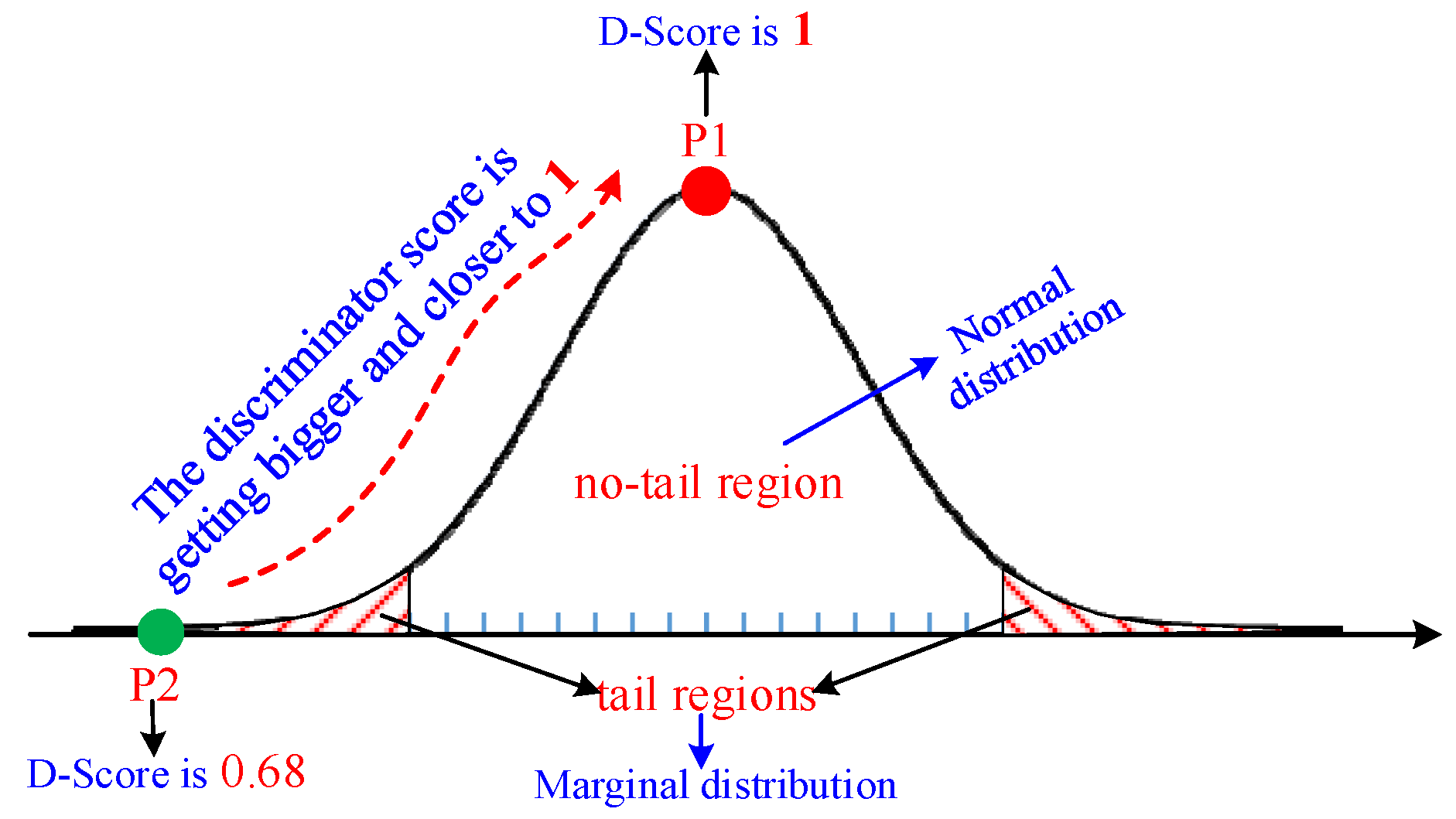
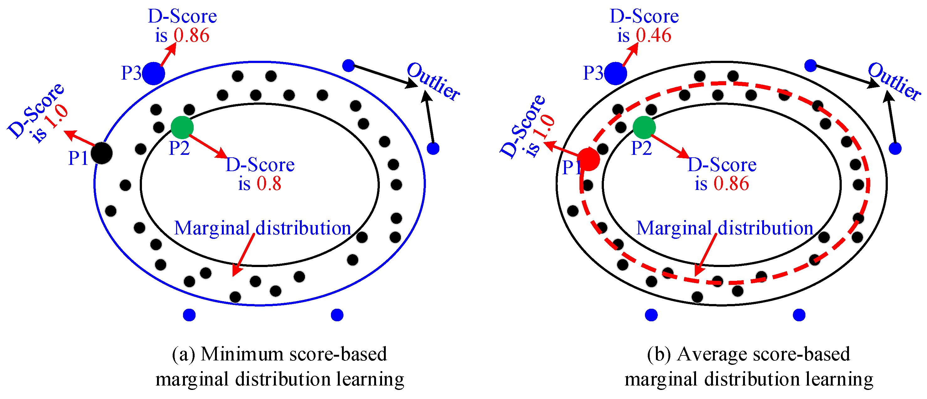
• A parameter-free dynamic strategy is designed to learn the marginal data distribution robustly and accurately through dynamic interaction between two GANs;
• Based on the learned marginal distribution and normal distribution, an anomaly score optimization strategy is used to enhance the accuracy and stability of anomaly detection from the feature space;
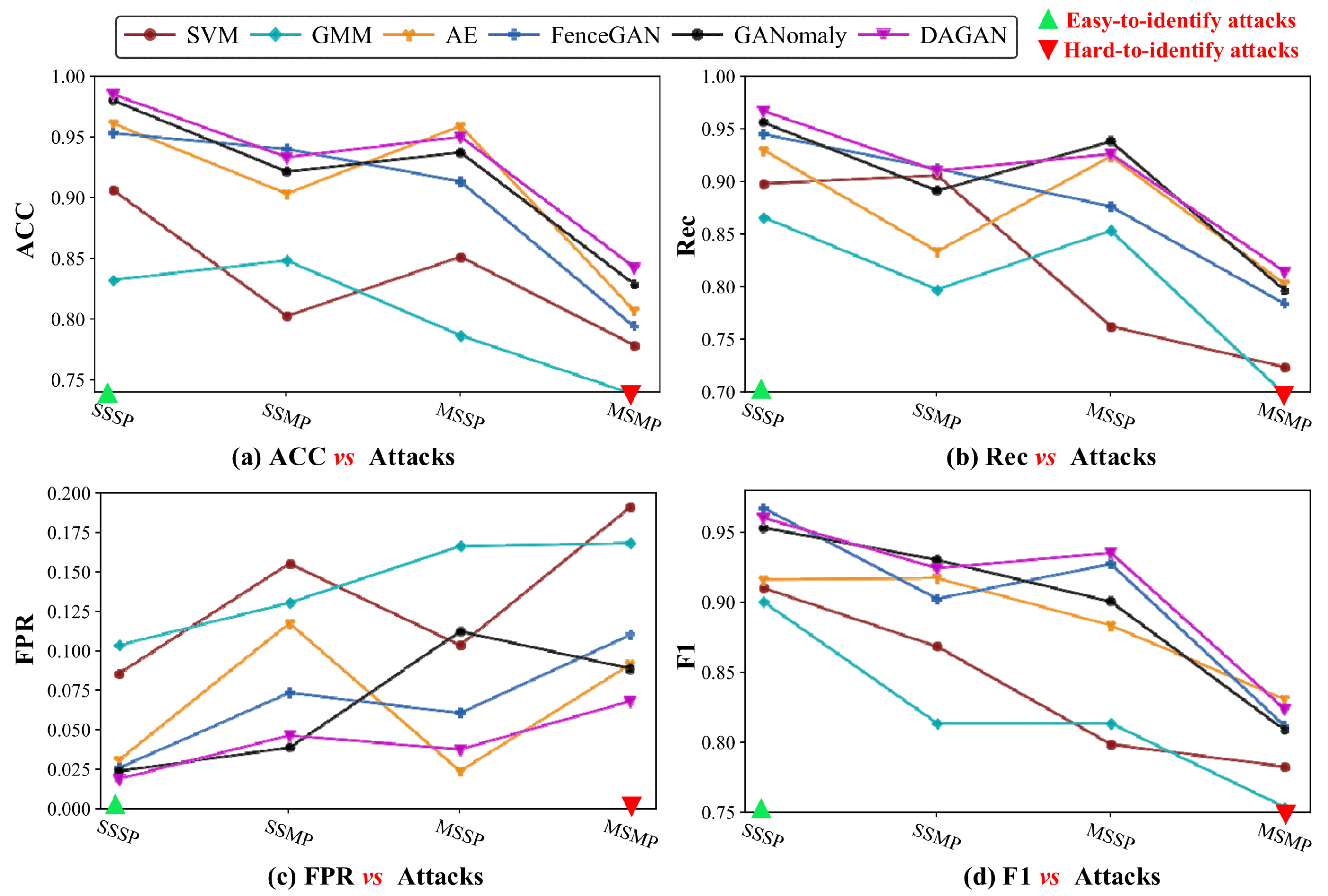
• Comparative experiments with five various networks on the DS2OST dataset and the SWAT dataset demonstrate the effectiveness of the DAGAN method.

The remainder of this paper is organized as follows: In Section 2, relevant papers on anomaly detection techniques in ICS are analyzed. Section 3 shows the preliminaries on GAN for anomaly detection. Section 4 presents the details of our DAGAN model. Our extensive experimental evaluation is stated in Section 5. Finally, the conclusion of this paper is presented.

2. Related Works

Taking network traffic and physical state as data, a large number of anomaly detection methods for ICS have been proposed [6,7,8,9,10]. These works are easily classified into the categories listed below.

• Statistical model-based methods make up the first category, with Gaussian mixture model (GMM) [11] and independent component analysis (ICA) [12] as typical representatives. The idea behind this is to build a statistical model of system operation, which is used to calculate the probability that the observed value of a random variable is within a certain range, and treat data that exceed a certain preset threshold as outlier. For example, Zhang et al. [13] combined GMM and linear discriminant analysis (LDA) to build a feature distribution model, and then used SVM to obtain the outliers in the smart meters data. Once models are built, they can be mathematically evaluated quickly and easily implemented. However, since they rely heavily on prior knowledge, the quality of the results produced is mostly unreliable in practical applications, and they are generally not suitable for multidimensional schemes. Xie et al. [14] used bilateral principal component analysis (B-PCA) to build a time series feature distribution model for the anomaly detection of network traffic. However, ICS has many resource-constrained heterogeneous devices, complex and diverse working environments, and a lot of noise, so it is very difficult to model accurately.
• Machine learning-based methods make up the second category, with support vector machine (SVM) [15] and regression model as typical representatives. The idea behind this is to use traditional machine learning methods to learn a latent feature distribution from normal data, so that data that do not satisfy this distribution are regarded as outliers. However, due to the complex and diverse operating environments of ICS, this method cannot accurately learn the deep features of normal data and is sensitive to high-dimensional noise. For example, Ma et al. [16] combined kernel Support Vector Machine (KSVM) and LDA to learn the latent normal feature distribution of network traffic, and then find anomalies. The efficacy of the proposed anomaly detection model in network traffic is great. However, it requires a pre-existed corpus for data transformation and model training. Poornima et al. [17] established the Online Locally Linear Weighted Projection Regression (OLWPR) model to achieve more accurate anomaly detection through online learning and data dimensionality reduction. The advantage of this is that there is no need to store all training data in node memory; only the model remains in the node and performs predictions. However, as the dimensionality of the data increases, the performance of these models degrades. Chen et al. [18] proposed an efficient NBAD algorithm based on deep belief networks (DBN) and long short-term memory networks (LSTM). This algorithm can accurately and quickly detect abnormal network behavior. Moreover, due to the feature extraction implemented by DBN and the light structure of the method, the time consumption of the training and detection processes is drastically reduced. However, it is not ideal for categories with few records in the dataset. Forestiero [19] proposed an activity footprint-based method to detect anomalies in IoT by exploiting a multiagent algorithm. This method can be used to dynamically handle information changes and exhibit adaptive behavior, and the proposed meta-heuristic is fully decentralized.
• Deep learning-based methods make up the third category, with auto-encoder, LSTM and Convolutional Neural Network (CNN) as typical representatives [20]. The basic idea behind this is to use deep neural networks to learn the deep features of normal data more accurately. For example, for discrete data, Kim et al. [21] constructed an auto-encoder model to map the data to a low-dimensional space to learn features, and then treat data that do not satisfy the features as anomalies. For time series data, Zhou et al. [22] used LSTM to learn deep features and anomaly detection. For image data, Zhang et al. [23] constructed a tensor-based convolutional neural network to learn the deep features of high-dimensional images and complete anomaly detection. Zhang et al. [24] combined a self-supervised learning module to learn general normal patterns and an adaptive memory fusion module to learn rich feature representations based on a convolutional auto-encoder structure. Although this method has good accuracy and robustness, it usually requires enough abnormal samples and heavily depends on the quality of training samples. It also has high time complexity.
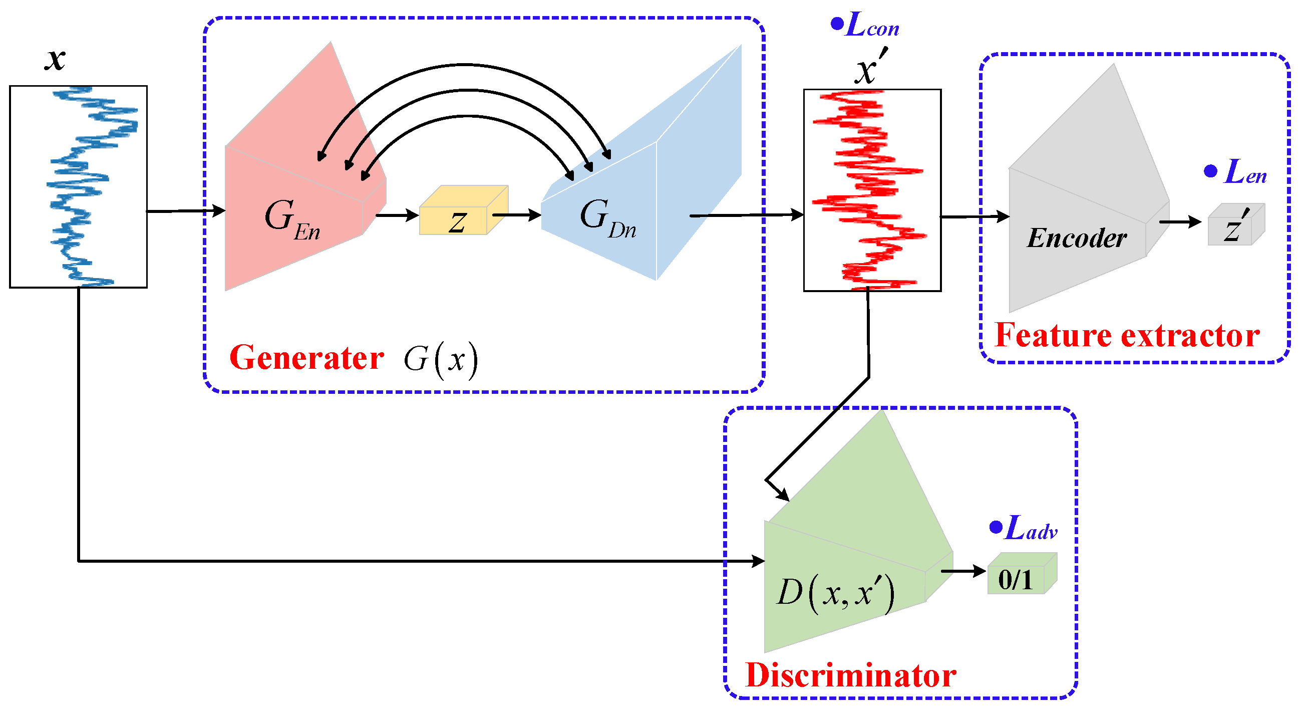
• In recent years, GAN-based anomaly detection has become a hot research topic. AnoGAN [25] in 2017 is the first work to use GAN to discover anomalies in high-dimensional image data. The basic process is to build a CNN as a generator G to generate an image with a Gaussian noise Z, and then build a discriminator D to accurately classify the generated image and the real image, and finally observe the difference between a test image and its generated image to determine whether this image is an outlier. However, this method requires a lot of training in the testing phase, so its time complexity is high. Zentai et al. [26] further constructed the BiGAN model to complete anomaly detection from both the feature space and the data space, which is more stable and takes less training time. The FenceGAN model [4] is proposed to utilize a modified GAN to learn the marginal distribution of real data for better anomaly detection. However, this method requires a preset threshold and is not robust. Since it is difficult to obtain abnormal samples, the GANomaly model [5] combines auto-encoder and GAN to design a novel “encoder–decoder–encoder” architecture, which can realize anomaly detection without abnormal samples. In addition, this model makes full use of the reconstruction ability of the auto-encoder and the feature learning ability of GAN, so as to achieve a more accurate anomaly detection from the feature space. However, this model cannot reconstruct the complex and variable high-dimensional data well. In summary, GAN has a strong ability to learn the potential distribution of high-dimensional data, and has good adaptability to strong noise, which is a better means to achieve accurate anomaly detection.

The data generated by the industrial control system are high dimensional and high noise, and they operate in a complicated operational environment with multiple operating modes. A comprehensive analysis of the above methods revealed that the GAN-based anomaly detection method is more suitable for use in the ICS. However, most of the previous GAN-based anomaly detection methods require anomaly data support for anomaly detection. However, these abnormal samples are difficult to obtain in practical applications. At the same time, none of these methods consider the “long-tailed distribution” phenomenon in ICS. Although FenceGAN takes into consideration the problem of “long-tailed distribution”, it also requires abnormal samples to participate in training, and requires many sensitive parameters, making it not robust and performing well in actual working conditions. Therefore, combined with the characteristics of ICS, we propose a more accurate and robust GAN-based anomaly detection approach.

As far as existing methods are concerned, the proposed method does not rely on abnormal samples at all and adapts to the high-dimensional and noisy data environment, making it especially suitable for systems such as ICS where it is difficult to obtain abnormal samples. It overcomes the problem of the general method often discriminating marginal samples as abnormal samples, so that the accuracy of anomaly detection tasks is significantly improved. In addition, the feature space provided by the auto-encoder guarantees the stability of anomaly detection results in the face of high-dimensional samples.

3. Preliminaries on GAN for Anomaly Detection

In this section, we first describe how the GAN model learns the distribution of latent data, and further elaborate the anomaly detection process based on the GANomaly model which is the inspired model of our work.

3.1. GAN-Based Unsupervised Normal Distribution Learning

Generative Adversarial Networks (GANs), developed and introduced in 2014, are a powerful class of neural networks that are used for learning the latent distribution of high-dimensional data. In GANs, there are two core components: generator G and discriminator D, both of which is a deep neural network as multilayer perceptron, convolutional neural network, etc. In the model, the generator G attempts to learn the latent distribution P_data(x) of the real data x, and generates a fake sample G(z) that satisfies the latent distribution based on a random noise z. The discriminator D takes the generated data G(z) and the real data x as input, and is responsible for binary classification to identify whether a sample is G(z) or x. In short, the goal of G is to confuse the fake with the real, and the goal of D is to distinguish between the real and fake. Therefore, the generator G and discriminator D constitute a min–max game. After multiple alternating trainings, the generator G and discriminator D gradually converge, and then the generator G has learned the latent distribution of the real data x.

The objective function of GAN model is as follows:

$$\underset{G}{\min }\underset{D}{\max }V\left(D,G\right)=\underset{x\sim P_{data}\left(x\right)}{E}\left[\log \left(D\left(x\right)\right)\right]+\underset{z\sim P_Z\left(z\right)}{E}\left[\log \left(1-D\left(G\left(z\right)\right)\right)\right]$$

(1)

where the G tries to minimize the distance between G(z) and x, and the D tries to maximize the distance between G(z) and x.

3.2. GANomaly-Based Anomaly Detection

A novel GAN-based anomaly detection model, called GANomaly, was proposed in 2018. This model ingeniously combines auto-encoder and GAN, to construct an “encoder–decoder–encoder” architecture. This new architecture does not rely on any abnormal samples; only normal samples are used for training. In addition, this architecture can provide accurate anomaly detection from the feature space. The pipeline of the GANomaly model is shown in Figure 1.

The GANomaly model consists of three sub-networks. The first sub-network is a generator G(x) consisting of an encoder G_En and a decoder G_Dn. It first encodes the input data x to obtain a low-dimensional vector z, and then uses the decoder to reconstruct the data x′ based on the z. The second sub-network is an encoding network, Encoder, which re-encodes the generated data x′ to obtain low-dimensional latent features z′. The third sub-network is the discriminator network D, which is responsible for the binary classification of the generated data x′ and the original data x.

Based on the above three sub-networks, the loss function of the GANomaly model is as follows:

(1) Adversarial Loss: If high-dimensional and variable data are directly measured, it is easy to cause mode collapse and gradient disappearance. Therefore, a feature matching loss is used instead of cross-entropy, and is defined as follows:

$$L_{adv}=\underset{x\sim P_X}{E}{\Vert f\left(x\right)-\underset{x\sim P_X}{E}f\left(G\left(x\right)\right)\Vert }_2$$

(2)

where the f(*) function is the output of an intermediate layer in D. The goal of G is to minimize the loss, and the goal of D is to maximize the loss.

(2) Contextual Loss:G can be optimized to learn the underlying distribution of the real data by minimizing the difference between the reconstructed data x′ and the original data x. It is defined as follows:

$$L_{con}=\underset{x\sim P_X}{E}{\Vert x-G\left(x\right)\Vert }_1$$

(3)

(3) Encoder Loss: This function minimizes the difference between the low-dimensional features of x′ and the low-dimensional features of x, ensuring that anomaly detection can be performed in the feature space. It is defined as follows:

$$L_{enc}=\underset{x\sim P_X}{E}{\Vert G_E\left(x\right)-E\left(G\left(x\right)\right)\Vert }_2$$

(4)

Therefore, the full loss function of the GANomaly model is computed as follows:

$$L=w_{adv}{L}_{adv}+w_{con}{L}_{con}+w_{enc}{L}_{enc}$$

(5)

where w_adv, w_con, and w_enc are the weights corresponding to the three loss functions.

After the GANomaly model is trained, the encoder G_En, the decoder G_Dn, and the reconstructed encoder, Encoder, can only identify the latent distribution of normal samples. Then, when an abnormal sample is input into the model, the encoder G_En and the decoder G_Dn will try to convert the abnormal sample into a normal sample G(x). This results in a significant difference between the low-dimensional feature z of the input x and the low-dimensional feature z′ of the generated x′. Therefore, the GANomaly model uses an anomaly score to measure this difference, defined as follows:

$$\mathrm{A}\left(x\right)={\Vert G_E\left(x\right)-E\left(G\left(x\right)\right)\Vert }_1$$

(6)

When the score of a sample is greater than a preset threshold μ, the sample is regarded as an outlier.

4. Dual Auto-Encoder GAN-Based Anomaly Detection for Industrial Control System (DAGAN)

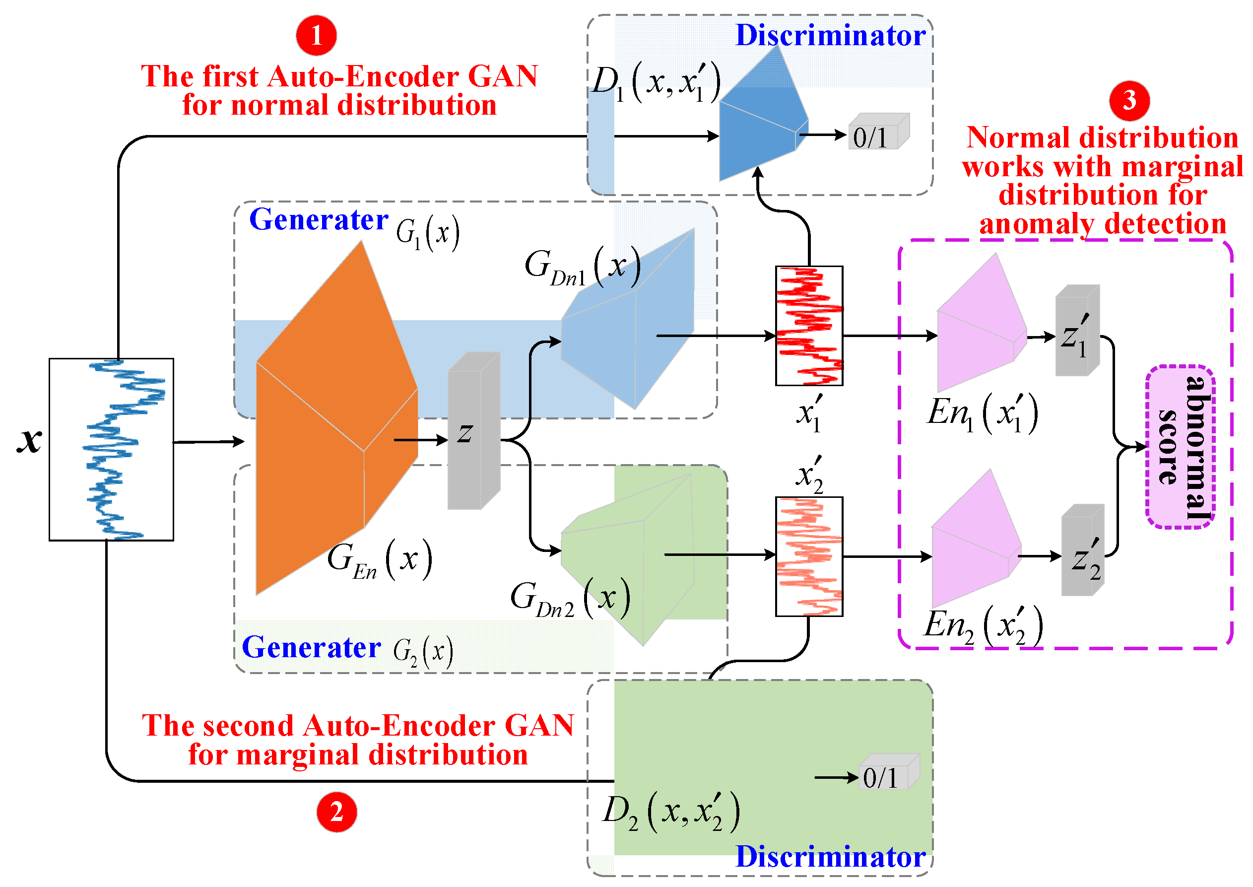
Industrial control systems (ICS) have some individual characteristics, which bring the following challenges to anomaly detection. (1) Most of the data collected in ICS are normal samples, and it is difficult to obtain abnormal samples. For wider applicability, an anomaly detection model needs to be able to perform accurate detection without relying on any anomalous samples. (2) The operation logic of ICS is relatively fixed, resulting in an obvious “long-tail” distribution of operating data, with a lot of data in dense areas and little data in marginal areas. This further leads to unseen marginal data being misidentified as outliers. (3) Affected by the complex working environment, the operating data in ICS have high noise. If anomaly detection is performed directly from the data space, the detection accuracy will inevitably decrease. Therefore, it is very necessary to perform anomaly detection from the feature space to improve the accuracy.

To solve the above challenges, inspired by GANomaly and FenceGAN models, a dual auto-encoder GAN-based anomaly detection model (DAGAN) is proposed in this paper for ICS. This model tries to use the reconstruction ability of auto-encoder and the feature learning ability of GAN to design an accurate and efficient deep model for anomaly detection of ICS that does not rely on any abnormal samples and can accurately identify real marginal samples.

4.1. DAGAN Model

4.1.1. Problem Definition

Our goal is to train an unsupervised deep model for anomaly detection using a dataset that is highly biased towards a particular class. In this dataset, the number of normal samples is much larger than the number of marginal samples, and also much larger than the number of abnormal samples. Furthermore, the unsupervised deep model does not require any anomalous samples during the training phase. The normal definition of this model is as follows:

We are given a large training set $D=\left\{x_1,x_2,\cdot \cdot \cdot ,x_M\right\}$ includes M samples, where the number of normal samples is much larger than the number of marginal samples. Additionally, a small test set $\hat{D}=\left\{\left(x_1,y_1\right),\left(x_2,y_2\right),\cdot \cdot \cdot ,\left(x_N,y_N\right)\right\}$ that includes N number samples which have normal samples, marginal samples and abnormal samples is given, where $y_i\in \left[0,1\right]$ indicates whether the sample is normal or abnormal. In addition, it must be ensured that the number of training samples is much larger than the number of test samples (M >> N).

Based on the given dataset, our idea is to first build a deep model to learn the latent distribution and marginal distribution of D at the same time. Then, each sample in the test set $\hat{D}$ is converted into a low-dimensional feature, and two new data are generated, one of which satisfies the learned normal distribution and the other satisfies the marginal distribution. Thereafter, each reconstructed data is re-encoded to calculate whether the low-dimensional features of the reconstructed data are the same as those of the original data. Eventually, the two anomaly scores are combined to finally decide whether a test sample is outlier.

4.1.2. Model Pipeline

The pipeline of our DAGAN model is shown in Figure 2. The DAGAN model tries to use only normal samples to learn an efficient neural network that can achieve accurate anomaly detection in the feature space, thereby reducing the false positive rate. Our DAGAN consists of three important components: the first GAN, the second GAN, and the feature extractor.

(1) The first GAN is an important component, which is responsible for helping the generator G₁ to learn the normal distribution of the training samples through adversarial training between the generator G₁ and the discriminator D₁. The generator G₁ consists of an encoder G_En and a decoder G_Dn1, both of which are multilayer perceptron networks. The encoder G_En is responsible for converting the normal data x into a low-dimensional vector z, and the decoder G_Dn1 is responsible for reconstructing the data $x_1^{\prime }$ according to z, and ensuring that the generated data $x_1^{\prime }$ are similar to the original data x. The discriminator D₁ is also a multi-layer perceptron, responsible for a binary classification of the original data x and the generated data $x_1^{\prime }$. Because a large number of samples in the training dataset are concentrated in the non-tail region, the latent distribution that can be learned by this GAN cannot cover the marginal distribution well, which will inevitably lead to poor discrimination scores for marginal samples.

(2) The second GAN is another important component that is responsible for learning the marginal distribution of the training samples to make up for the shortcomings of the first GAN. The generator G₂ is also an auto-encoder architecture, consisting of an encoder G_En and decoder G_Dn1. The purpose of G₁ and G₂ sharing the encoder G_En is to ensure that the generated data come from the same low-dimensional latent feature z. G_Dn2 has the same multilayer perceptron structure as G_Dn1, but each learns different parameters. The goal of G_Dn2 is to generate a marginal sample $x_2^{\prime }$ based on z. Likewise, the discriminators D₂ and D₁ have the same neural network structure but different parameters.

(3) The feature extractor is the third component, which is responsible for converting the data generated by the two GANs into low-dimensional features again, and then performing more accurate anomaly detection from the low-dimensional feature space, so as to avoid the influence of noise in the high-dimensional data space and improve the stability of the model. The feature extractor consists of encoder En₁ and encoder En₂. The En₁ is responsible for encoding $x_1^{\prime }$, and ensuring that the resulting low-dimensional feature $z_1^{\prime }$ is the same as the low-dimensional feature z of the original data x. Likewise, En₂ is responsible for encoding $x_2^{\prime }$ and ensuring that the $z_1^{\prime }$ is the same as the z. Finally, the low-dimensional vectors $z_1^{\prime }$ and $z_2^{\prime }$ are combined to achieve more accurate anomaly detection.

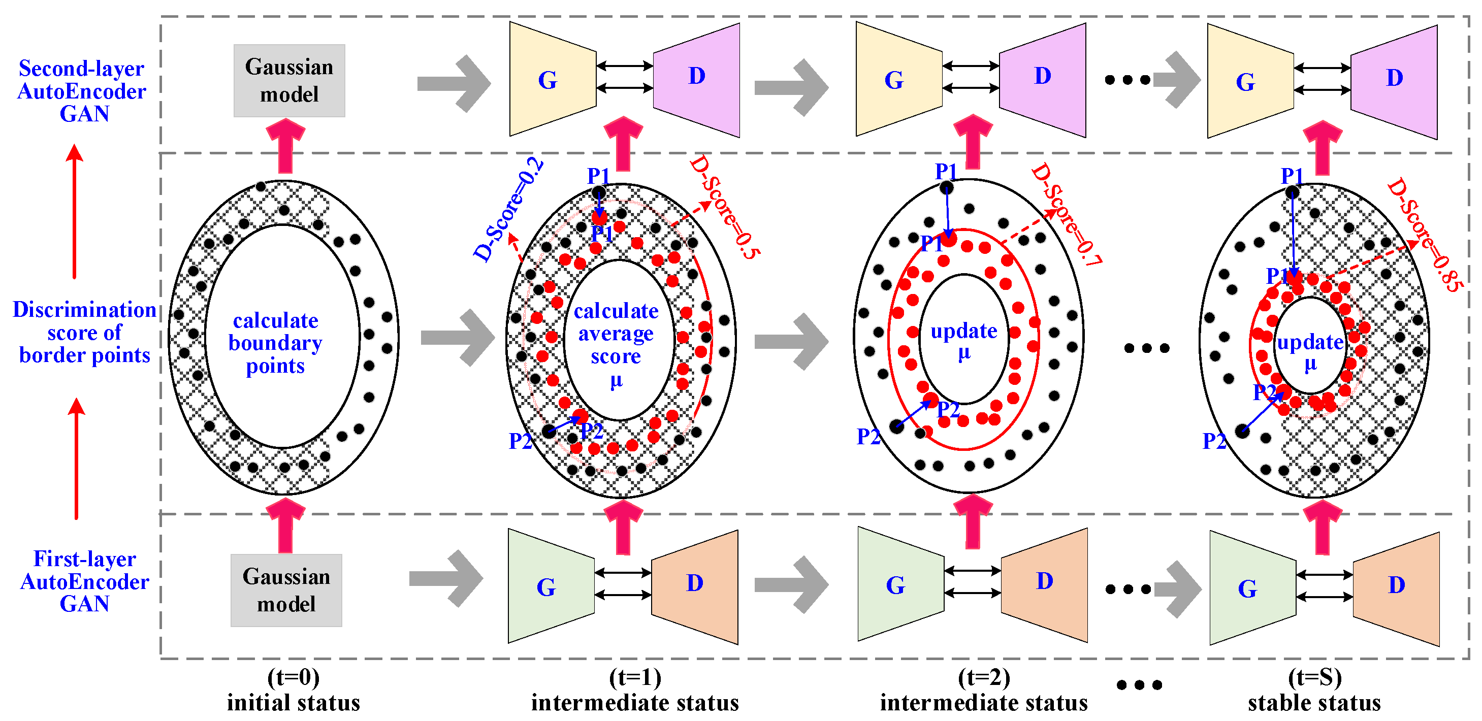
4.1.3. Parameter-Free Marginal Distribution Learning

For the DAGAN model to work efficiently, a key problem needs to be solved: how do we learn the marginal distribution directly from the training samples?

To solve this problem, a discriminator score-based strategy inspired by the FenceGAN model is used in this paper to learn the marginal distribution of the training dataset. The basic idea is that when a large number of normal samples (non-tail data) and a small number of marginal samples (tail data) are used to train the discriminator in GAN, the discriminator will try to accurately identify the normal samples with a score of 1. At the same time, a small number of marginal samples reach a score less than 1, such as 0.8. That is to say, the discriminator score can be used as an indicator to measure whether a sample is a marginal sample, as shown in Figure 3. In the figure, a long-tail data distribution is presented, where the non-tail region represents the normal distribution with a very large area, and the tail regions on both sides represent the marginal distribution with a very small area. If a discriminator in GAN is used to identify the data of this distribution, the red point P1 has a score of 1, and the green point P2 has a score of 0.68. Moreover, as the data points are closer to the center of the data distribution, the discriminator score (D-Score) gets larger and closer to 1. In other words, the smaller the D-Score of a training sample, the more likely that training sample is in the marginal distribution. Based on the above idea, the FenceGAN model introduces a preset threshold μ to treat all samples with a discrimination score less than u as marginal samples. Through the adversarial training between the generator and the discriminator in the GAN, the generator can generate marginal samples with a D-Score close to μ, so as to learn the marginal distribution of the training dataset.

However, different datasets in ICS have different characteristics, and their preset thresholds μ must be different. In addition, it is difficult to know which marginal samples are collected from the real training samples. These limitations seriously affect the wide application of the FenGAN model. To enhance robustness and applicability, this paper tries to design a parameter-free marginal distribution learning strategy based on discriminator score, which can quickly and efficiently learn the marginal distribution of any industrial control system. To achieve this goal, three difficulties need to be solved:

(1) The first difficulty is how to automatically calculate the threshold μ without any supervision information. The easiest way is to take the minimum discriminant score (D-Score) in the dataset as μ. However, this strategy is prone to giving high scores to many outliers close to the marginal distribution, resulting in these outliers being misjudged, as shown in Figure 4a. In the figure, all black points are marginal points and the region where they are located is marginal distribution, and all blue points are outliers close to marginal distribution. When the discriminator uses the minimum score (blue oval circle) as the learning criterion, the discriminator will assign a higher score to the point closer to the blue oval. For example, P1 has a score of 1.0, P3 has a score of 0.86, and P2 has a score of only 0.8. This results in the blue outlier P3 being misjudged as a normal sample. To solve this difficulty, the average value of the scores of multiple marginal points is used as the value of the parameter μ in this paper, as shown in Figure 4b. In this figure, the red dotted ellipse is the average of the scores of multiple marginal points, which is used to help the discriminator learn the marginal distribution. Based on the new threshold μ, the blue anomaly point P3 will have a small score of 0.46, and the green point P2 will have a larger score of 0.86. The above strategy can help to better learn the marginal distribution of the for any industrial control dataset, avoid the misjudgment of outliers near the marginal region, and improve the accuracy of the model.

(2) The second problem is how to determine the number of marginal samples in the dataset. To calculate the parameter μ, we need to determine the number of marginal points in the dataset. However, the industrial control system is difficult to model, so it is difficult to judge whether there are marginal samples in the large collected samples, and it is even more difficult to determine which ones are marginal samples. To solve this difficulty, this paper uses the Gaussian distribution to approximate the long-tail distribution of the real dataset. In the Gaussian distribution, the area of the [c − 2σ, c + 2σ] is 95%, where c is the mean and σ is the standard deviation. For simplicity, this paper uses 5% as the cutoff to determine the number of marginal samples in a training dataset. The main reasons for using this strategy are as follows: Firstly, marginal samples are usually a very small proportion of the training dataset. Secondly, the average of the scores of multiple marginal samples is set as the parameter μ. Therefore, when the number of marginal points is large, a few more points and a few less points have little effect on the average of all points. Thirdly, when the proportion of marginal points is less than or more than 5%, those points that are over-computed or under-computed have very close D-Scores and do not have much impact on the average of all points. Therefore, based on this strategy, it is very easy to obtain the marginal points for any dataset.

(3) The third question is how to quickly calculate the discriminator score (D-Score) for each marginal point. To calculate the parameter μ, we also need to know the discriminator score for each marginal point. The most direct and simple way is to train a binary classifier on the real dataset, then score all samples, and regard the samples with the smallest score as the marginal samples. However, this strategy requires additional training of a binary classifier, which is very time consuming. To solve this difficulty, this paper tries to use the process of learning normal distribution in the DAGAN model to help quickly calculate the D-Score for marginal points. The idea is that each time the first GAN is trained, the discriminator in the first GAN is used to calculate the D-Score of the marginal samples in the second GAN. In the first stage, the discriminator in the first GAN is not stable, so the obtained D-Scores of marginal points will be biased. As the number of training increases, the discriminator in the first GAN will gradually stabilize and the D-Scores of these marginal points in the second GAN will gradually converge. Based on this strategy, we can not only accurately obtain the D-Score of each marginal sample in the second GAN, but also greatly reduce the training time of our DAGAN model.

In summary, a discriminator score-based parameter-free marginal distribution learning strategy is developed in this paper. The process of this strategy is shown in Figure 5, which includes the following three steps. Step 1 is initialization (t = 0). The weights of the two GANs in the DAGAN model are randomly initialized and take 5% of the total number of samples in the training set as the number of marginal samples (MN). Step 2 is dynamic interaction between two GANs (t = 1 to t = S). At t = 1, the first GAN is trained with the training dataset. After the training is completed, the discriminator D₁ is used to score all samples, the top-MN samples with the smallest scores are seen as marginal samples to calculate the μ, and the μ as a parameter is inputted into the second GAN. Based on the μ, the second GAN starts training to learn marginal distribution. Therefore, the first GAN and the second GAN will be alternately trained for multiple rounds (t = 2 and t = S − 1). After each round of training of the first GAN, the scores of all marginal samples are updated, and then the threshold μ of the second GAN is also updated. As the discriminator D₁ in the first GAN gradually converges, the scores of all marginal samples will also gradually converge. When t = S, the first GAN converges, the scores of all marginal samples are fixed, and the threshold μ of the second GAN is also fixed. Step 3 involves more training for the second GAN. When the first GAN converges, the second GAN must not have converged due to the dynamic change of the threshold μ. Therefore, more training of the second GAN is required until the second GAN converges. When the second GAN converges, the generator G₂ in the second GAN has learned the marginal distribution of the dataset, and can generate marginal sample with the score of μ.

4.2. Model Training

Inspired by the GANomaly and FenceGAN models, the loss function and training process of our DAGAN model were optimized, as shown in the next section.

4.2.1. Training Objectives

(1) 

The first GAN sub-network

Generator G₁. The G₁ consists of an encoder G_En and a decoder G_Dn1, which aims to learn the normal distribution of the training dataset. Moreover, the G₁ is also directly concatenated with the feature extractor to form an encoder–decoder–encoder structure (G_En-G_Dn1-En₁). Therefore, the loss function of the generator G₁ consists of three parts:

• Adversarial Loss: This function is responsible for making the generated sample as real as possible, so that the discriminator D₁ cannot correctly identify whether the samples are real or generated. The loss function is defined as follows:

$$L_{adv}^{G_1}=\frac{1}{N}{\displaystyle \sum _{i=1}^N\left[\log \left(1-D_1\left(G_1\left(x\right)\right)\right)\right]}$$

(7)

By minimizing the above adversarial loss, the generator G₁ can learn the normal distribution of the training dataset.

• Reconstruction Loss: The purpose is to ensure that G_Dn1 can accurately learn the normal distribution of the training dataset by making the sample $x_1^{\prime }$ reconstructed by G_Dn1 as similar as possible to the original sample x. The loss function is defined as follows:

  $$L_{rec}^{G_1}=\frac{1}{N}{\displaystyle \sum _{i=1}^N{\Vert x-G_1\left(x\right)\Vert }_1}$$

  (8)

• Encoder Loss: This function is responsible for ensuring that the low-dimensional feature $z_1^{\prime }$ of $x_1^{\prime }$ obtained by the encoder En₁ is as similar as possible to the low-dimensional feature z of the original sample x. The loss function is defined as follows:

  $$L_{enc}^{G_1}=\frac{1}{N}{\displaystyle \sum _{i=1}^N{\Vert G_{En}\left(x\right)-E{n}_1\left({x^{\prime }}_1\right)\Vert }_2}$$

  (9)

In summary, the training objective of the generator G₁ (G_En-G_Dn1-En₁) of the first GAN is as follows:

$$L_{G1}=w_{adv}^{G_1}{L}_{adv}^{G_1}+w_{rec}^{G_1}{L}_{rec}^{G_1}+w_{enc}^{G_1}{L}_{enc}^{G_1}$$

(10)

where $w_{adv}^{G_1}$, $w_{rec}^{G_1}$, and $w_{enc}^{G_1}$ are the weights corresponding to the three loss functions.

The above loss function will help the first GAN to learn the normal distribution of the training dataset, so that it cannot only reconstruct the real samples, but also accurately get the low-dimensional features of the real samples.

Discriminator D₁: The discriminator D₁ of the first GAN is a binary classifier with a multi-layer perceptron structure. It takes real samples and generated samples of G₁ as input, and the goal is to accurately identify whether the input sample is a generator sample or a real sample. The loss function is defined as follows:

$$L_{D1}=\frac{1}{N}{\displaystyle \sum _{i=1}^N\left[-\log \left(D_1\left(x\right)\right)-\log \left(1-D_1\left(G_1\left(x\right)\right)\right)\right]}$$

(11)

(2) 

The second GAN sub-network

Generator G₂. The G₂ consists of an encoder G_En and a decoder G_Dn2. Moreover, the G₂ is also directly concatenated with the En₂ to form an encoder–decoder–encoder structure (G_En-G_Dn2-En₂). In addition, G_Dn2 and En₂ share the same neural network structure as G_Dn1 and En₁. The goal of Generator G₂ in the second GAN is to learn the marginal distribution of the training dataset. Therefore, the loss function of the generator G₂ includes four parts:

• Adversarial Loss: The purpose is to help the generator G₂ generate data with the discriminator score μ, so as to learn the marginal distribution of the real training set. The loss function is defined as follows:

$$L_{adv}^{G_2}=\frac{1}{N}{\displaystyle \sum _{i=1}^N\left[\log \left(\mu -D_2\left(G_2\left(x\right)\right)\right)\right]}$$

(12)

where μ is the average of the scores of all marginal samples, and the detailed calculation process is described in Section 4.1.3.

• Dispersion Loss: The purpose is to supervise the data generated by G₂ to be as evenly dispersed as possible in the marginal distribution, rather than fixed in some small regions. The loss function is defined as follows:

$$\begin{array}{l}{L}_{dis}^{G_2}=\frac{1}{\frac{1}{N}{\displaystyle \sum _{i=1}^N\left({\Vert G_2\left(x\right)-AVG\Vert }_2\right)}}\\ AVG=\frac{1}{N}{\displaystyle \sum _{i=1}^N{G}_2\left(x\right)}\end{array}$$

(13)

where AVG is the centroid of all generated data.

• Context Loss: This function is responsible for ensuring that the similarity between the marginal samples generated by G₂ and the normal samples generated by G₁ in the feature space is the same as the similarity between the discriminator scores. The loss function is defined as follows:

$$\begin{array}{l}{L}_{con}^{G_2}=\frac{1}{N}{\displaystyle \sum _{i=1}^N\left({\Vert si{m}_{dis}-si{m}_{fea}\Vert }_1\right)}\\ si{m}_{dis}={\Vert D_1\left(x\right)-D_1\left(G_2\left(x\right)\right)\Vert }_1\\ si{m}_{fea}={\Vert G_{En}\left(G_1\left(x\right)\right)-G_{En}\left(G_2\left(x\right)\right)\Vert }_2\end{array}$$

(14)

• Encoder Loss: This function is responsible for ensuring that the low-dimensional feature $z_2^{\prime }$ of $x_2^{\prime }$ obtained by the encoder En₂ is as similar as possible to the low-dimensional feature z of the original sample x. The loss function is defined as follows:

  $$L_{enc}^{G_2}=\frac{1}{N}{\displaystyle \sum _{i=1}^N{\Vert G_{En}\left(x\right)-E{n}_2\left({x^{\prime }}_2\right)\Vert }_2}$$

  (15)

In summary, the training objectives of the generator G₂ in the second GAN composed of “G_En-G_Dn2-En₂” are as follows:

$$L_{G2}=w_{adv}^{G_2}{L}_{adv}^{G_2}+w_{dis}^{G_2}{L}_{dis}^{G_2}+w_{con}^{G_2}{L}_{con}^{G_2}+w_{enc}^{G_2}{L}_{enc}^{G_2}$$

(16)

where $w_{adv}^{G_2}$, $w_{dis}^{G_2}$, $w_{con}^{G_2}$, and $w_{enc}^{G_2}$ are the weights corresponding to the four loss functions.

Discriminator D₂: The discriminator D₂ of the second GAN is also a binary classifier with the same structure as D₁. It takes real samples and generated samples of G₂ as input, and the goal is to accurately identify whether the input sample is a generator sample or a real sample. The loss function is defined as follows:

$$L_{D2}=\frac{1}{N}{\displaystyle \sum _{i=1}^N\left[-\log \left(D_2\left(x\right)\right)-\log \left(\mu -D_2\left(G_2\left(x\right)\right)\right)\right]}$$

(17)

where μ is the average of the scores of all marginal samples, and the detailed calculation process is described in Section 4.1.3.

4.2.2. Training Process

Based on the above loss functions, the training process of our DAGAN model is an alternate iterative training between two GANs. The detailed process is as follows: First, the weights of our DAGAN model are randomly initialized. Second, the first GAN starts being trained. The generator G₁ and the encoder En₁ are fixed, and a batch of samples with label 0 is generated by G₁. The generated samples with label 0 and real samples with label 1 are input into the discriminator D₁ for training to complete a binary classification. After the discriminator D₁ is trained, fix D₁ and use the real samples to train G₁ and En₁. According to the encoder–decoder–encoder pipeline, each real sample x is encoded by G_En into a low-dimensional feature z, anthen z is reconstructed by G_Dn1 into $x_1^{\prime }$, and finally $x_1^{\prime }$ is encoded by En₁ into a low-dimensional feature $z_1^{\prime }$. According to the loss function (Equation (10)), the parameters of G_En, G_Dn1 and En₁ are updated. Third, start training the second GAN after training the first GAN. The discriminator D₁ of the first GAN is used to score all real samples to get the marginal samples and calculate the threshold μ. According to the threshold μ, the discriminator D₂ and generator G₂ of the second GAN are trained alternately. The training process is the same as the first GAN, the loss function of the D₂ is Formula (17), and the loss function of the generator G2 is Formula (16). Finally, the first GAN and the second GAN are trained alternately for multiple rounds. After each round of training of the first GAN, the marginal samples are recalculated and the threshold μ is updated. Based on the updated μ, the second GAN is trained. When two GANs converge, the training of our DAGAN model ends.

4.3. Anomaly Detection

When the training of our DAGAN model is complete, by considering both the normal distribution and the marginal distribution, the model can detect whether a test sample is an outlier or not from the feature space.

A test sample $\hat{x}$ is first fed into the first GAN to obtain its low-dimensional feature z. Second, z is reconstructed into a new sample ${{\hat{x}}^{\prime }}_1$ according to the normal distribution learned by G₁. Finally, ${{\hat{x}}^{\prime }}_1$ is encoded again by En₁ as a low-dimensional feature $z_1^{\prime }$. Therefore, the first anomaly score measures the similarity between two features z and $z_1^{\prime }$, defined as:

$$\begin{array}{l}{S}_1={\Vert G_{En}\left(\hat{x}\right)-En\left(G_1\left(\hat{x}\right)\right)\Vert }_2\\ Scor{e}_1=\frac{S_1-S_1^{Min}}{S_1^{Max}-S_1^{Min}}\end{array}$$

(18)

When the test sample $\hat{x}$ is a normal sample, Score₁ is small and close to 0. When the test sample $\hat{x}$ is a marginal sample, Score₁ is large. When the test sample $\hat{x}$ is outlier, Score₁ is very large.

According to the first anomaly score, marginal samples and outliers cannot be well identified, which may easily lead to the misjudgment of marginal samples. For this, the test sample $\hat{x}$ is again fed into the second GAN and reconstructed to generate marginal samples ${{\hat{x}}^{\prime }}_2$ according to the marginal distribution learned by G₂. To compare $\hat{x}$ and ${{\hat{x}}^{\prime }}_2$ from the feature space, the output features of an intermediate layer in discriminator D₂ are used. Therefore, the first anomaly score measures the similarity between two features of $\hat{x}$ and ${{\hat{x}}^{\prime }}_2$, defined as:

$$\begin{array}{l}{S}_2={\Vert f\left(\hat{x}\right)-f\left(G_2\left(\hat{x}\right)\right)\Vert }_2\\ Scor{e}_2=\frac{S_2-S_2^{Min}}{S_2^{Max}-S_2^{Min}}\end{array}$$

(19)

When the test sample $\hat{x}$ is a normal sample, Score₂ is small. When the test sample $\hat{x}$ is a marginal sample, the Score₂ is close to 0. When the test sample $\hat{x}$ is an outlier, the Score₂ is large.

Combining the above two scores, the final anomaly score of our DAGAN model is defined as follows:

$$A\left(\hat{x}\right)=\left(1-\gamma \right)Scor{e}_1+\gamma Scor{e}_2$$

(20)

where γ is a hyper-parameter with a value of [0–1], representing the importance of Score₂.

Based on the above anomaly score, we can quickly identify whether a test sample is an outlier, and greatly reduce the probability of unseen marginal samples being misjudged. Because when both normal samples and marginal samples are tested, the anomaly score is smaller. Conversely, when anomalous samples are tested, the anomaly score becomes significantly larger.

5. Experimental Evaluation

5.1. Experimental Dataset

In this paper, two publicly available industrial control system datasets are selected to train and verify our DAGAN model. The detailed descriptions of the two datasets are as follows:

(1) DS2OS dataset: This dataset is an open source and publicly accessible dataset, which was collected from Kaggle (https://www.kaggle.com/francoisxa/ds2ostraffictraces or https://github.com/fkie-cad/ipal_datasets, accessed on 13 December 2021) provided by Pahl. This dataset is an IoT testbed dataset generated by Distributed Smart Space Orchestration System (DS2OS). This dataset contains 357,952 samples, of which the number of normal samples is 347,935, and the number of abnormal samples is 10017. For each sample, there are 13 features. All abnormal samples can be classified into the following 7 types of attacks: Denial of Service (DoS), Data Type Probing (DP), Malicious Control (MC), Malicious Operation (MO), Scan (SC), Spying (SP), and Wrong Setup (WS). More specifically, 5780 samples belong to the DoS attack, 342 samples belong to the DP attack, 889 samples belong to the MC attack, 805 samples belong to the MO attack, 1547 samples belong to the SCAN attack, 532 samples belong to the SP attack, and 122 samples belong to the WS attack.

(2) SWaT dataset: This dataset is an open source and publicly accessible dataset (https://itrust.sutd.edu.sg/itrust-labs-home/itrust-labs_swat/ or https://github.com/fkie-cad/ipal_datasets, accessed on 17 December 2021). This dataset was generated by a water treatment testbed. This dataset is collected from 51 sensors and executor within 11 days. In the 11 days, the testbed was running normally in the first 7 days, and various attacks were randomly injected into the testbed in the last 4 days. This dataset contains 946,722 samples, each with 103 features. This dataset contains 4 types of attacks: Single-Stage Single-Point (SSSP), Single-Stage Multi-Point (SSMP), Multi-Stage Single-Point (MSSP), and Multi-Stage Multi-Point (MSMP) attacks. More specifically, the number of all attacks is 36, of which the number of SSSP attacks is 23, the number of SSMP attacks is 6, the number of MSSP attacks is 4, and the number of MSMP attacks is 3. The duration of each attack is between 1 and 60 min.

For simplicity, 20,000 normal samples in DS2OS dataset are used as the training set in this paper, 1500 normal samples and 350 abnormal samples are used as the test set (50 samples for each attack). For the SWaT dataset, 15,000 normal samples are used as the training set in this paper, 700 normal samples and 160 abnormal samples are used as the test set (40 samples for each attack).

5.2. Experimental Setup

Comparison Algorithms: To effectively verify the performance of our DAGAN model, five representative anomaly detection algorithms are chosen as competitors. All comparison algorithms are listed in

Table 1. Comparison algorithms.

Algorithm	Full Name	Implement
SVM [15]	Anomaly-based Intrusion Detection in Industrial Data with SVM and Random Forests.	Python
GMM [11]	Unusual Activity and Anomaly Detection in Surveillance Using GMM-KNN Model.	Python
AE [27]	Anomaly Detection for Industrial Control System based on Auto-encoder Neural Network.	Python
FenceGAN [4]	Fence GAN: Towards Better Anomaly Detection.	Python
GANomaly [5]	GANomaly: Semi-Supervised Anomaly Detection via Adversarial Training.	Python
DAGAN	Dual Auto-Encoder GAN-Based anomaly detection for industrial control system.	Python

, where the SVM is a machine learning-based anomaly detection method, GMM is a Gaussian mixture model-based method, AE is an auto-encoder neural network-based method, FenceGAN and GANomaly both are GAN-based anomaly detection methods. For all comparison algorithms, recommended values of all parameters are used to obtain the best experimental results.

Evaluation metrics: In this paper, Accuracy (ACC), Recall (Rec), False positive rate (FPR), and F1-Score (F1) are selected as evaluation indicators to evaluate the quality of anomaly detection. They are defined as follows:

$$ACC=\frac{TP+TN}{TP+FN+FP+TN}$$

(21)

$$Rec=\frac{TP}{TP+FN}$$

(22)

$$FPR=\frac{FP}{FP+TN}$$

(23)

$$F1=2\times \frac{\left(\frac{TP}{TP+FN}\right)\times \left(\frac{TP}{TP+FP}\right)}{\left(\frac{TP}{TP+FN}+\frac{TP}{TP+FP}\right)}$$

(24)

where True Positive (TP) is a positive sample predicted to be positive, True Negative (TN) is a negative sample predicted to be negative, False Positive (FP) is a negative sample predicted to be positive, and False Negative (FN) is a positive sample predicted to be negative.

Experimental Platform: A normal PC server (ThinkPad L490) is used as the experimental platform. The server is equipped with an 8-core i7 CPU, 16 GB of main memory, and Windows 10 operating system. The DAGAN model is programmed with Python and runs with Spyder as an IDE. For the other algorithms, the official python implementation is downloaded from the websites of the corresponding authors.

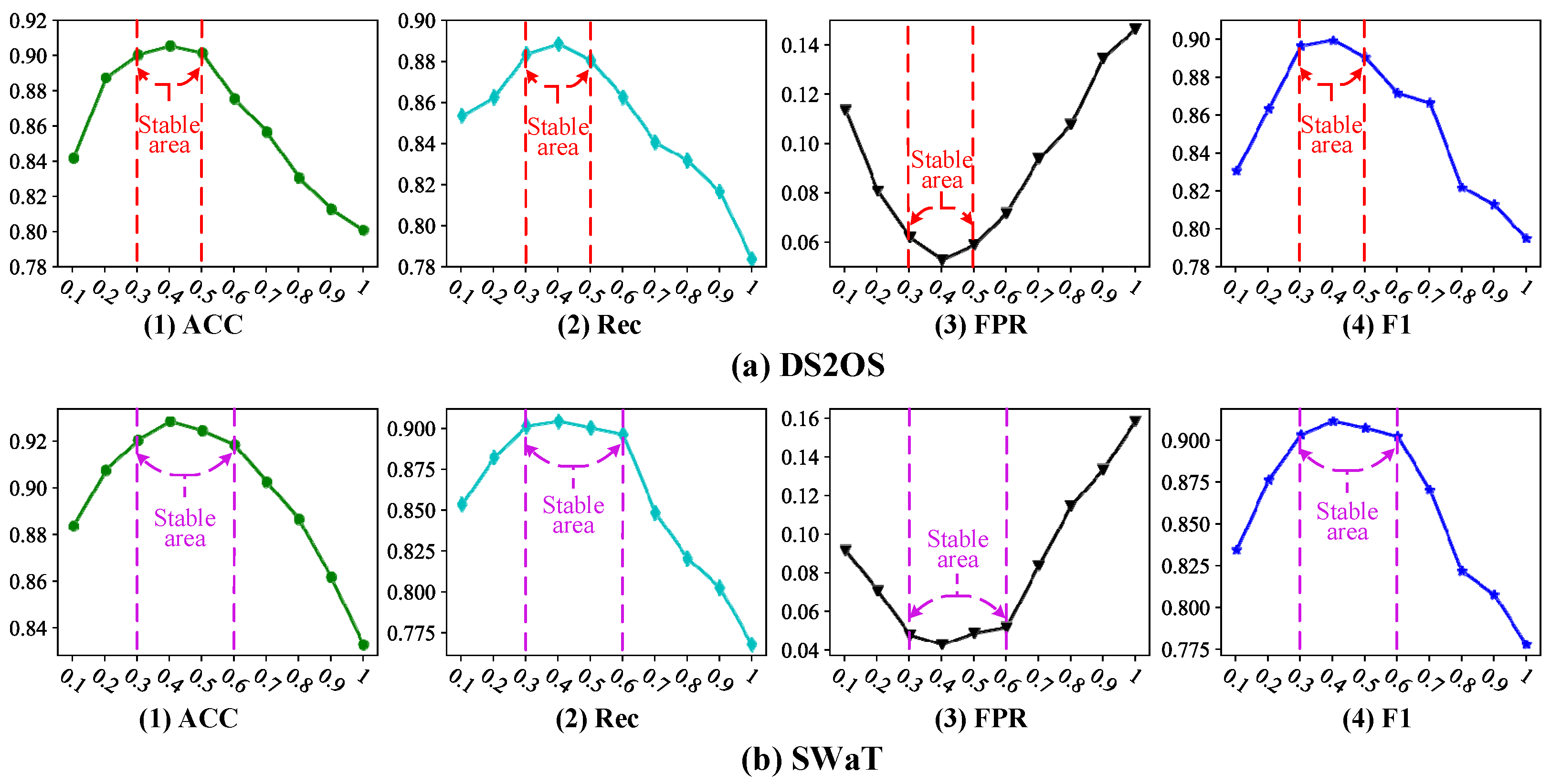
5.3. Sensitivity Analysis of the Hyper-Parameter γ

The first experimental objective is to verify the sensitivity of the hyper-parameter γ and find a stable region for different ICS datasets. The hyper-parameter γ is defined to measure the ratio of the marginal distribution score (Formula (19)) to the overall anomaly score (Formula (20)) for a test sample. The value range of hyper-parameter γ is [0–1]. The larger the value, the larger the proportion of the marginal distribution score in the overall anomaly score. This further means that a test sample with high marginal distribution score is more likely to be judged as an outlier. To get the stable region of the hyper-parameter γ, we performed two experiments based on four evaluation metrics of ACC, Rec, FPR, and F1. (1) The first experiment uses DS2OS as the experimental data and uses the training set and test set given in Section 5.1 to train and optimize the DAGAN model. Because the DS2OS dataset contains 7 kinds of attacks, 7 test sets consisting of 30 abnormal samples and 50 normal samples are established, each test set contains only one attack and is different from other test sets. By gradually increasing γ from 0 to 1, we try to find the stable region of parameter γ by observing the change of the average value of 7 test sets on 4 evaluation metrics, as shown in Figure 6a. (2) Similar to the first experiment, the second experiment uses SWaT dataset to train and optimize the DAGAN model. Additionally, 4 test sets consisting of 20 abnormal samples and 40 normal samples are established. The experimental results are shown in Figure 6b.

Figure 6 plots the ACC, Rec, FPR and F1 trend lines of the DAGAN model on the DS2OS and SWaT datasets under different hyper-parameters γ. From the figure, we can find the following observations. (1) As the hyper-parameter γ increases from 0 to 0.3, the anomaly detection performance (ACC, Rec, FPR and F1) of our DAGAN model improves rapidly. For example, for the SWaT dataset, the FPR value is only 0.09 at γ = 0.1, but the FPR value is 0.04 at γ = 0.3. (2) As hyper-parameter γ increases from 0.5 to 1.0 (or from 0.6 to 1.0), the ACC, Rec, FPR and F1 performance of our DAGAN model degrades rapidly on the DS2OS dataset (or on the SWaT dataset). Such as, for DS2OS dataset, the F1 value is 0.87 at γ = 0.6, but the F1 value is only 0.8 at γ = 0.8. (3) As hyper-parameter γ increases from 0.3 to 0.5 (or from 0.3 to 0.6), the performance of our model varies slightly and is relatively stable on the DS2OS dataset (or on the SWaT dataset). For example, the Rec value on the SWaT dataset is almost the same at γ = 0.3 and γ = 0.4, both around 0.9. Additionally, the ACC value on the DS2OS dataset is almost the same at γ = 0.4 and γ = 0.5, both around 0.92.

In summary, the [0.3–0.6] is a stable region of hyper-parameters γ for the different ICS datasets. In later experiments, the hyper-parameter γ was set to 0.4.

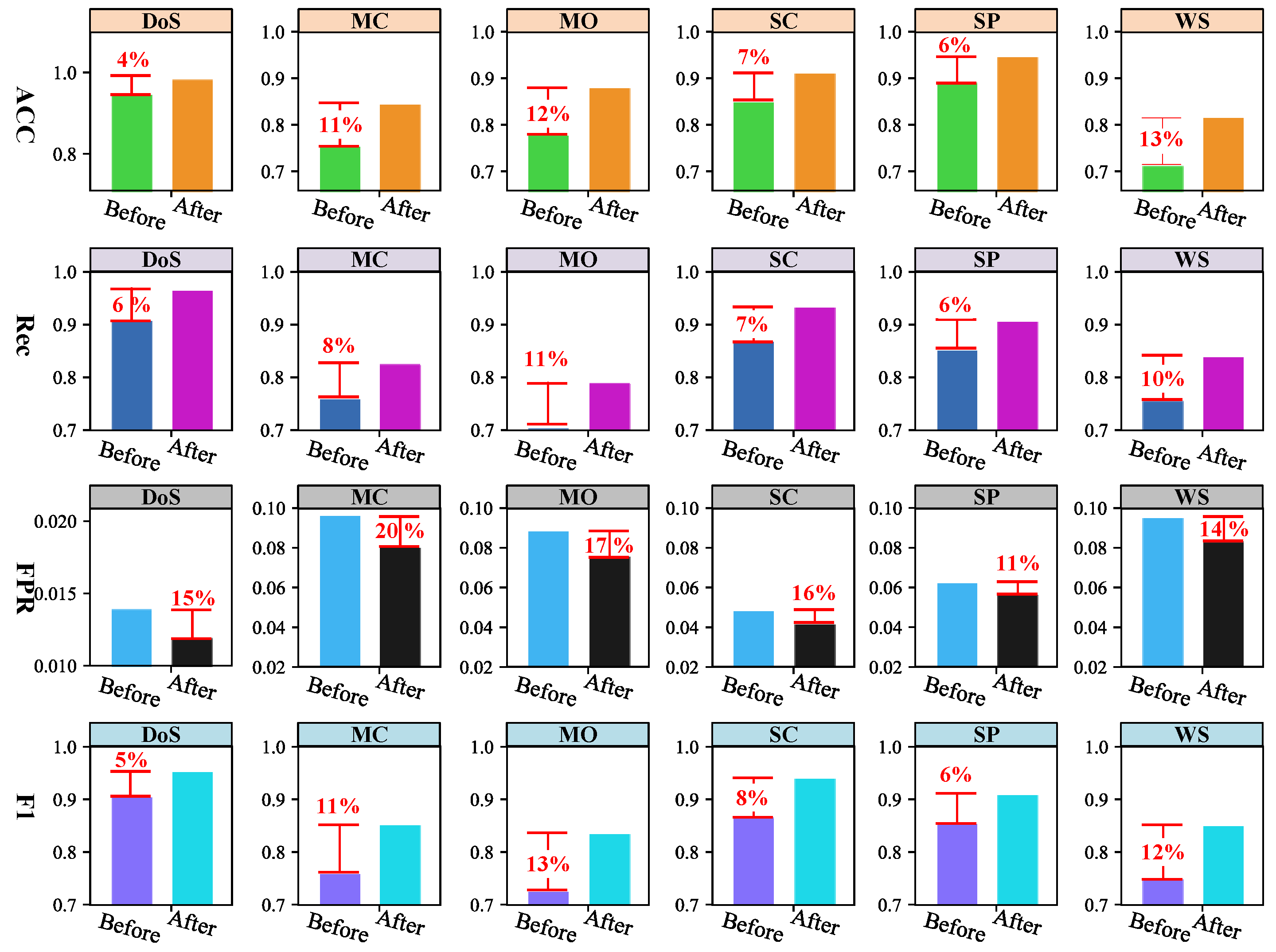
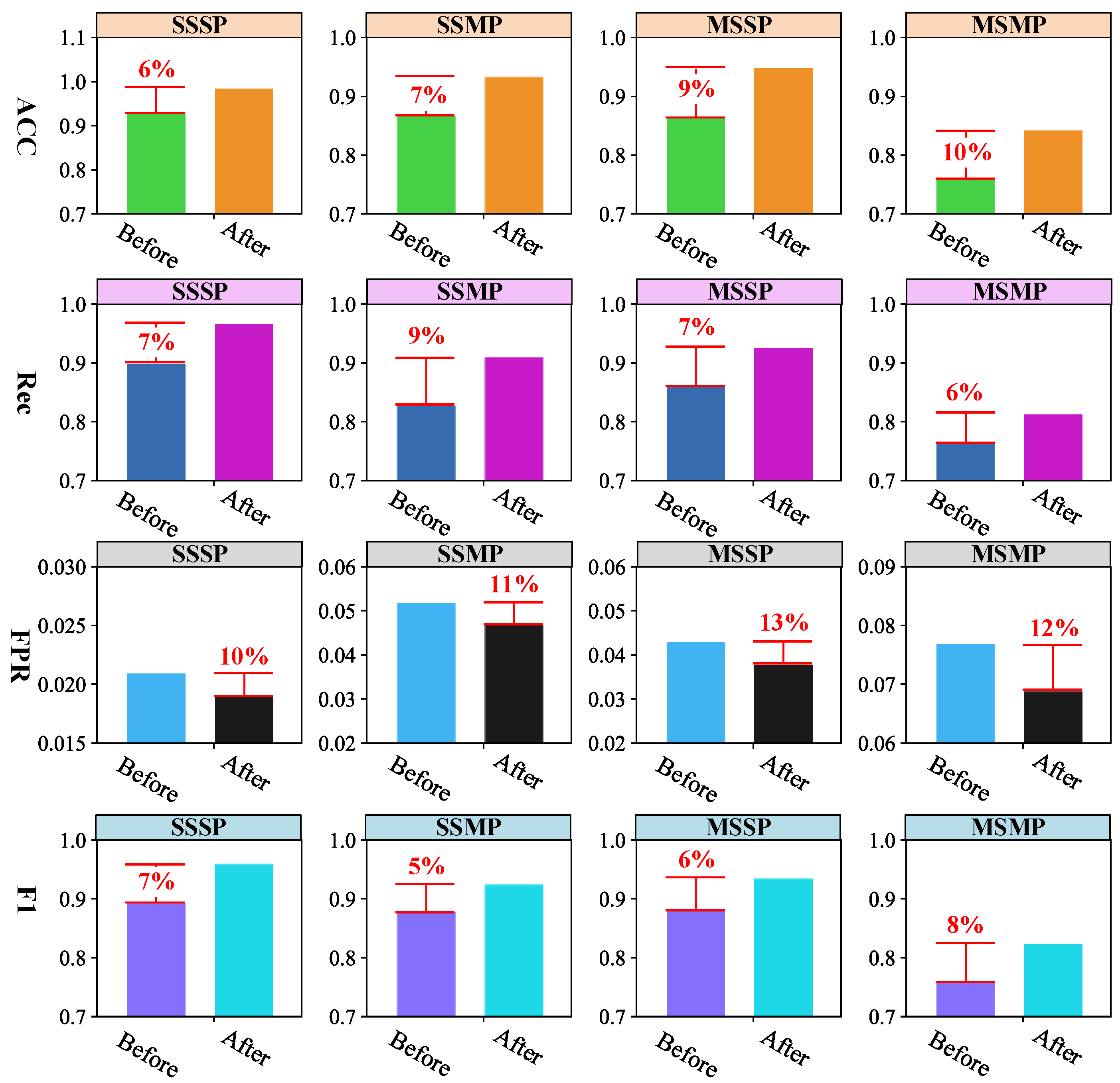
5.4. Performance Analysis of Optimization Strategy for the Marginal Distribution Learning

The second experimental objective is to verify the effectiveness of optimization strategy for the marginal distribution learning. In this paper, an optimization strategy is proposed to achieve parameter-free marginal distribution learning, aiming to improve the robustness of our model. Furthermore, in the optimization strategy, the average of the discriminator scores of multiple marginal nodes is used instead of the minimum value for better learning the marginal distribution. To verify the effectiveness of our strategy, the minimum value-based strategy is used as another competitor. In this experiment, we try to analyze the anomaly detection performance based on two strategies for verifying the effectiveness of our strategy, as shown in Figure 7 and Figure 8. The ACC, Rec, FPR and F1 are used as evaluation metrics, and DS2OS and SWaT are chosen as the experimental datasets. For two datasets, multiple samples of each attack are combined with multiple normal samples to establish a test set. Therefore, there are 6 test sets for DS2OS (DP attack is ignored for easy drawing) and 4 test sets for SWaT.

In Figure 7, the first row plots the ACC performance of two strategies on 6 test sets, the second row plots the Rec performance, the third row plots the FPR performance, and the four row plots the F1 performance, respectively. On each test set, the first bars represent the anomaly detection performance of the minimum value-based marginal distribution learning strategy, the second bars represent the performance of our optimization strategy, and the red numbers are the values of performance optimization. From the figure, the following observations are easily obtained. (1) For the ACC, our strategy shows good optimization performance on 6 test sets, with an average optimization rate of 9%. Moreover, the optimization performance of our strategy is stronger for the test set with lower detection accuracy. For example, when the detection accuracy on the DoS test set reaches 97%, and the optimized value of our strategy is only 4%. When the detection accuracy on the WS test set is only 80%, the optimized value of our strategy reaches 13%. (2) For the Rec, our strategy also shows good performance, with an average optimization value of 8%. (3) For the FPR, the optimization performance of our strategy is better than that of the ACC, Rec, and F1, with an average optimization value of 15%. For example, the optimized value is 20% on the MC test set, the value is 17% on the MO test set, and the value is 16% on the SC test set. (4) For the F1, the average optimized value of our strategy is 9%. In addition, the lower the detection accuracy, the stronger the optimization ability of our strategy.

Figure 8 further plots the performance analysis of two optimization strategies on the SWaT dataset. Same as Figure 7, the first, second, third and fourth rows in this figure show the ACC, Rec, FPR and F1 performance of the two strategies on the 4 test sets, respectively. From Figure 8, it is easy to get some patterns. (1) Our strategy can effectively improve the performance of anomaly detection. For example, the average optimization value on the ACC is 8%, the value on the Rec is 7%, the value on the FPR is 11%, and the value on the F1 is 6%. Moreover, the anomaly detection performance of ACC, Rec, and F1 exceeds 95% on the SSSP test set, exceeds 90% on the SSMP test set. (2) The lower the performance of ACC, Rec, FPR, and F1 on a test set, the stronger the optimization ability of our strategy. Such as, on the SSSP test set, the accuracy of anomaly detection (ACC, Rec, and F1) exceeds 95%, the optimized value of our strategy is 6% on the ACC, 7% on the Rec, 7% on the F1. However, on the MSMP test set, accuracy of anomaly detection (ACC, Rec, and F1) is only around 83%, the optimized value of our strategy is 10% on the ACC, 12% on the FRP, and 8% on the F1.

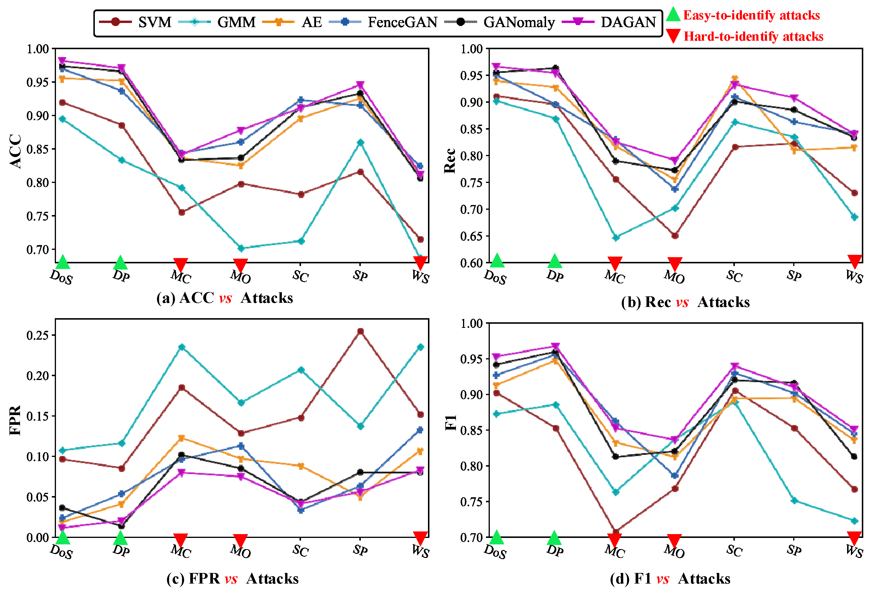
5.5. Performance Analysis of Anomaly Detection

The third experimental objective is to verify the anomaly detection performance of our DAGAN algorithm, and to further compare the GANomaly and DAGAN models. In this experiment, SVM, GMM, AE, FenceGAN, GANomaly are used as competitors, the ACC, Rec, FPR and F1 are used as evaluation metrics, and DS2OS and SWaT are chosen as the experimental datasets. For the DS2OS dataset, 7 test sets are established. Each test set consists of 30 abnormal samples and 50 normal samples, and each test set contains only one attack that is different from other test sets. For SWaT dataset, 4 test sets are established, and each test set consists of 20 abnormal samples and 40 normal samples.

Figure 9 plots the anomaly detection accuracy of 6 models on the 7 test sets of the DS2OS, where Figure 9a plots the ACC results, Figure 9b plots the Rec results, Figure 9c plots the FPR results, and Figure 9d plots the F1 results. In the figure, the green triangle indicates that the detection accuracy on this verification set is high, indicating that the attack is easy to detect, abbreviated. The green triangle indicates that the detection accuracy in the test set is high, which implies that the attack in this test set is easy to be detected, simply called easy-to-identify attack. On the contrary, the red triangle indicates that the detection accuracy in the test set is low, which implies that the attack in this test set is difficult to be detected, simply called hard-to-identify attack. Form the figure, some observations are obtained. (1) For four metrics (ACC, Rec, FPR and F1), the 6 models have different performances, and the trend lines of these model have surged drastically. Comparing the 6 models, DAGAN, GANomaly, FenceGAN, and AE have the best anomaly detection results, SVM and GMM are the worst. Moreover, the stability of our DAGAN model is better than other models. (2) For easy-to-identify attacks with green triangles (DOS and DP), the detection accuracy of the DAGAN, GANomaly, FenceGAN and AE models is very high (The average value of ACC, Rec, or F1 is close to 0.95), and the performance of the four models is very close. (3) For hard-to-identify attacks with red triangles (MC, MO and WS), there are differences between the detection accuracy of the DAGAN, GANomaly, FenceGAN and AE models, and our model has a slight advantage. (4) Focusing only on the GANomaly and DAGAN models, the performance of the DAGAN model is better than that of the GANomaly model, especially for hard-to-detect attacks.

Figure 10 further presents the anomaly detection performance of 6 models on 4 test sets of the SWaT from ACC, Rec, FPR, and F1 metrics. In the figure, the 6 models have achieved good results on different test sets, and the average values of the ACC, Rec and F1 are greater than 0.82. However, the performance of these 6 models varies greatly, with better performance on some test sets and poor performance on other test sets. More specifically, we can get the following observations. (1) For the ACC, the anomaly detection accuracy of the 6 models on the 4 test sets fluctuate sharply, and the stability is very poor. For example, the AE model performs poorly on SSMP and MSMP, but performs well on MSSP. Comparing these 6 models, DAGAN, GANomaly, FenceGAN and AE models have the best performance and stability. The SVM and GMM models have the worst performance and poor stability. (2) For the Rec, the curves of these 6 models are very uneven. Among them, DAGAN and GANomaly are the best, FenceGAN and AE are second, SVM and GMM are the worst. (3) For the FPR, the DAGAN and FenceGAN have better stability than other models. Moreover, for the 6 models, the advantage of our DAGAN model on hard-to-identify attack (red triangle) is stronger than on easy-to-identify attack (green triangle). (4) For the F1, the 6 models are more stable than the Rec and FPR metrics. Comparing the 6 models, DAGAN, GANomaly and FenceGAN models have better performance than the AE, GMM and SVM models. Authors should discuss the results and how they can be interpreted from the perspective of previous studies and of the working hypotheses. The findings and their implications should be discussed in the broadest context possible. Future research directions may also be highlighted.

6. Conclusions

To find outliers more robustly and accurately in industrial control systems, this paper developed a dual auto-encoder GAN-based anomaly detection model called DAGAN. First, this model only uses normal samples to train an “encoder-decoder-encoder” architecture, which can achieve anomaly detection without any abnormal samples and enhances the applicability of the model. Second, a dynamic optimization strategy is designed to be incorporated into the DAGAN model to better learn the marginal distribution of training data and reduce the misjudgment of marginal samples. Third, considering both normal distribution and marginal distribution, an optimized anomaly score is defined to judge whether a sample is outlier, so as to improve the accuracy of anomaly detection. Extensive experimental results on DS2OS and SWaT datasets demonstrate the effectiveness of our DAGAN model’s optimization strategy for marginal distribution learning. The advantages of the DAGAN model are further demonstrated by comparative experiments with other state-of-the-art methods.

In future work, the aim is to extend the method to the multi-class case to achieve multi-class anomaly detection. Since the anomaly category is difficult to obtain, the method proposed in this paper can be as a front-stage technique to extract sample features. Then, the model to be studied in the next step can achieve multi-classification anomaly detection from two aspects: (1) in the case of zero-shot, the category of attacks is detected by clustering methods [28,29] according to the extracted features by the method in this paper; (2) in the case of few-shot, the GAN model proposed in this paper is used to supplement and balance the number of small samples in each category, so as to improve the accuracy of existing methods for multi-classification.

References

1. Asghar, M.R.; Hu, Q.; Zeadally, S. Cybersecurity in industrial control systems: Issues, technologies, and challenges. Comput. Netw. 2019, 165, 106946. [Google Scholar] [CrossRef]
2. Rubio, J.E.; Alcaraz, C.; Roman, R.; Lopez, J. Current cyber-defense trends in industrial control systems. Comput. Secur. 2019, 87, 101561. [Google Scholar] [CrossRef]
3. Feng, C.; Palleti, V.R.; Mathur, A.; Chana, D. A Systematic Framework to Generate Invariants for Anomaly Detection in Industrial Control Systems. In Proceedings of the Network and Distributed Systems Security (NDSS) Symposium 2019, San Diego, CA, USA, 24–27 February 2019. [Google Scholar] [CrossRef]
4. Ngo, P.C.; Winarto, A.A.; Kou, C.K.L.; Park, S.; Akram, F.; Lee, H.K. Fence GAN: Towards better anomaly detection. In Proceedings of the 2019 IEEE 31St International Conference on Tools with Artificial Intelligence (ICTAI), Portland, OR, USA, 4–6 November 2019; pp. 141–148. [Google Scholar]
5. Akcay, S.; Atapour-Abarghouei, A.; Breckon, T.P. Ganomaly: Semi-supervised anomaly detection via adversarial training. In Computer Vision—ACCV 2018; Springer: Cham, Switzerland, 2018; pp. 622–637. [Google Scholar]
6. Rousseeuw, P.J.; Hubert, M. Anomaly detection by robust statistics. Wiley Interdiscip. Rev. Data Min. Knowl. Discov. 2018, 8, e1236. [Google Scholar] [CrossRef] [Green Version]
7. Pang, G.; Shen, C.; Cao, L.; Hengel, A.V.D. Deep learning for anomaly detection: A review. ACM Comput. Surv. (CSUR) 2021, 54, 1–38. [Google Scholar] [CrossRef]
8. Erhan, L.; Ndubuaku, M.; Di Mauro, M.; Song, W.; Chen, M.; Fortino, G.; Bagdasar, O.; Liotta, A. Smart anomaly detection in sensor systems: A multi-perspective review. Inf. Fusion 2021, 67, 64–79. [Google Scholar] [CrossRef]
9. Cook, A.A.; Misirli, G.; Fan, Z. Anomaly Detection for IoT Time-Series Data: A Survey. IEEE Internet Things J. 2019, 7, 6481–6494. [Google Scholar] [CrossRef]
10. Thudumu, S.; Branch, P.; Jin, J.; Singh, J.J. A comprehensive survey of anomaly detection techniques for high dimensional big data. J. Big Data 2020, 7, 1–30. [Google Scholar] [CrossRef]
11. Priya, G.S.; Latha, M.; Manoj, K.; Prakash, S. Unusual Activity And Anomaly Detection In Surveillance Using GMM-KNN Model. In Proceedings of the 2021 Third International Conference on Intelligent Communication Technologies and Virtual Mobile Networks (ICICV), Tirunelveli, India, 4–6 February 2021; pp. 1450–1457. [Google Scholar]
12. Zhang, R.; Dai, H. Independent component analysis-based arbitrary polynomial chaos method for stochastic analysis of structures under limited observations. Mech. Syst. Signal Processing 2022, 173, 109026. [Google Scholar] [CrossRef]
13. Zhang, L.; Wan, L.; Xiao, Y.; Li, S.; Zhu, C. Anomaly Detection method of Smart Meters data based on GMM-LDA clustering feature Learning and PSO Support Vector Machine. In Proceedings of the 2019 IEEE Sustainable Power and Energy Conference (ISPEC), Beijing, China, 21–23 November 2019; pp. 2407–2412. [Google Scholar]
14. Xie, K.; Li, X.; Wang, X.; Cao, J.; Xie, G.; Wen, J.; Zhang, D.; Qin, Z. On-Line Anomaly Detection With High Accuracy. IEEE/ACM Trans. Netw. 2018, 26, 1222–1235. [Google Scholar] [CrossRef]
15. Anton, S.D.D.; Sinha, S.; Schotten, H.D. Anomaly-based intrusion detection in industrial data with SVM and random forests. In Proceedings of the 2019 International Conference on Software, Telecommunications and Computer Networks (SoftCOM), Split, Croatia, 19–21 September 2019; pp. 1–6. [Google Scholar]
16. Ma, Q.; Sun, C.; Cui, B.; Jin, X. A novel model for anomaly detection in network traffic based on kernel support vector machine. Comput. Secur. 2021, 104, 102215. [Google Scholar] [CrossRef]
17. Poornima, I.G.A.; Paramasivan, B. Anomaly detection in wireless sensor network using machine learning algorithm. Comput. Commun. 2020, 151, 331–337. [Google Scholar] [CrossRef]
18. Chen, A.; Fu, Y.; Zheng, X.; Lu, G. An efficient network behavior anomaly detection using a hybrid DBN-LSTM network. Comput. Secur. 2022, 114, 102600. [Google Scholar] [CrossRef]
19. Forestiero, A. Metaheuristic algorithm for anomaly detection in Internet of Things leveraging on a neural-driven multiagent system. Knowl.-Based Syst. 2021, 228, 107241. [Google Scholar] [CrossRef]
20. Zhou, F.; Huang, Z.; Zhang, C. Carbon price forecasting based on CEEMDAN and LSTM. Appl. Energy 2022, 311, 118601. [Google Scholar] [CrossRef]
21. Kim, S.J.; Jo, W.Y.; Shon, T. APAD: Autoencoder-based payload anomaly detection for industrial IoE. Appl. Soft Comput. 2020, 88, 106017. [Google Scholar] [CrossRef]
22. Zhou, X.; Hu, Y.; Liang, W.; Ma, J.; Jin, Q. Variational LSTM Enhanced Anomaly Detection for Industrial Big Data. IEEE Trans. Ind. Inform. 2020, 17, 3469–3477. [Google Scholar] [CrossRef]
23. Zhang, L.; Cheng, B. Transferred CNN Based on Tensor for Hyperspectral Anomaly Detection. IEEE Geosci. Remote Sens. Lett. 2020, 17, 2115–2119. [Google Scholar] [CrossRef]
24. Zhang, Y.; Wang, J.; Chen, Y.; Yu, H.; Qin, T. Adaptive Memory Networks with Self-supervised Learning for Unsupervised Anomaly Detection. IEEE Trans. Knowl. Data Eng. 2022, 1. [Google Scholar] [CrossRef]
25. Schlegl, T.; Seeböck, P.; Waldstein, S.M.; Schmidt-Erfurth, U.; Langs, G. Unsupervised Anomaly Detection with Generative Adversarial Networks to Guide Marker Discovery. In International Conference on Information Processing in Medical Imaging; Springer: Cham, Switzerland, 2017; pp. 146–157. [Google Scholar]
26. Zenati, H.; Foo, C.S.; Lecouat, B.; Manek, G.; Chandrasekhar, V.R. Efficient gan-based anomaly detection. arXiv 2018, arXiv:1802.06222. [Google Scholar]
27. Wang, C.; Wang, B.; Liu, H.; Qu, H. Anomaly Detection for Industrial Control System Based on Autoencoder Neural Network. Wirel. Commun. Mob. Comput. 2020, 2020, 8897926. [Google Scholar] [CrossRef]
28. Eskandarnia, E.; Al-Ammal, H.M.; Ksantini, R. An embedded deep-clustering-based load profiling framework. Sustain. Cities Soc. 2021, 78, 103618. [Google Scholar] [CrossRef]
29. Ma, J.W.; Leite, F. Performance boosting of conventional deep learning-based semantic segmentation leveraging unsupervised clustering. Autom. Constr. 2022, 136, 104167. [Google Scholar] [CrossRef]
Figure 1. The pipeline of GANomaly model.
Applsci 12 04986 g001
Figure 2. The pipeline of DAGAN model.
Applsci 12 04986 g002
Figure 3. Correlation of discriminator score with marginal distribution.
Applsci 12 04986 g003
Figure 4. Optimization strategy for threshold μ.
Applsci 12 04986 g004
Figure 5. Discriminator score-based marginal distribution learning.
Applsci 12 04986 g005
Figure 6. Sensitivity analysis of hyper-parameter γ.
Applsci 12 04986 g006
Figure 7. Performance analysis of two optimization strategies on DS2OS dataset.
Applsci 12 04986 g007
Figure 8. Performance analysis of two optimization strategies on SWaT dataset.
Applsci 12 04986 g008
Figure 9. Anomaly detection performance analysis of multiple models on DS2OS dataset.
Applsci 12 04986 g009
Figure 10. Anomaly detection performance analysis of multiple models on SWaT dataset.
Applsci 12 04986 g010