A Dynamic Hysteresis Model for TMR-Current Sensors Based on Probability Estimation of Hysteresis Operator and Its Switching Time

Abstract

Hysteresis is one of the main factors affecting the measurement accuracy of TMR sensors, especially in dynamic measurements. The commonly used Preisach hysteresis compensation model has some problems, such as complex modeling and difficulty in accurately measuring the step time, resulting in low accuracy in dynamic measurements. In this paper, considering the distribution characteristics of the conversion time of the hysteresis operator in dynamic measurements, a dynamic hysteresis model based on the probability estimation of the hysteresis operator and its conversion time is proposed. Compared with the existing methods, this method only needs to calculate the distribution of the sensor hysteresis operator to realize the calculation of hysteresis characteristics without a physical model or fitting algorithm. It has good generalization performance and a corresponding fast speed. In the test of two typical TMR sensors, compared with the transmission Preisach model, the maximum error of this method is reduced by 46.7%, the variance can be reduced by 90.2%, and the average value can be reduced by 65.1%.

1. Introduction

The giant magnetoresistance effect (GMR) was discovered by Fert et al. [1] and Grünberg et al. [2] in 1988. Because of its excellent characteristics, it is applied in many fields, such as medicine [3], aviation [4], nondestructive testing [5], magnetic storage [6], electric power [7,8], and automobiles [9], etc. Its discoverers also won the 2007 Nobel Prize. There are four kinds of GMR, namely magnetic tunnel structure, spin valve structure, multilayer structure, and granular alloy structure. The tunnel magnetoresistive sensor (TMR) has attracted widespread attention because of its high sensitivity, suppression of temperature drift, self-compensation, and wide linear range.

One of the limitations of TMR sensors in the high-frequency field is their low accuracy, and one of the main reasons for the low accuracy is hysteresis. Hysteresis can be divided into static (quasi-static) hysteresis and dynamic hysteresis. Static hysteresis mainly refers to the hysteresis that occurs when working at an extremely low frequency regardless of time. Dynamic hysteresis refers to the hysteresis at a higher frequency, which is related to frequency or input change rate.

Currently, there are mainly two methods to reduce the influence of hysteresis. One is to reduce the hysteresis by designing the sensor’s manufacturing process, structure, materials, or hardware circuit. For example, AlOx barrier [10], spin direction and shape [11], self-bias sandwich structure [12], external bias structure [13], and so on. However, most of these methods are complex, expensive, involve high power consumption, and are not easy to apply.

Another method is to model the hysteresis characteristics of the sensor and to compensate for the measurement results in order to reduce the influence of hysteresis. Currently, there are mainly two kinds of models. One is the black-box model, which does not explain the input–output relationship but directly fits it. It includes the models based on empirical formulas and those based on machine learning. Empirical formula models mainly include the use of spline functions [14], rational polynomial [15], arctangent function [16], etc. However, the scope of the application of empirical formulas models is relatively small. The machine learning method includes the Recurrent Neural Network Model [17], artificial neural network [18], NARMAX [19], etc. These methods can solve the problem of model mapping to a certain extent, but it is difficult to realize and the cost is high.

The other is the white-box model. A series of models based on the Preisach model is the most representative. For example, the JA model [20] and KP model [21]. However, the accuracy of these models is not high, and the measurement is complex, which cannot effectively solve the hysteresis problem. Therefore, studying the hysteresis problem further is necessary to obtain a more efficient and easy-to-implement modeling method.

In the previous study of this research group, we thought that the change of the first-order rotation curve of TMR has a strong correlation with the probability distribution of the hysteresis operator. We analyzed the probability distribution characteristics of the hysteresis operator. Then, we regarded the output of the sensor as the ratio of the hysteresis operator satisfying certain conditions of all hysteresis operators. Moreover, we obtained the fast and accurate calculation of the static hysteresis characteristics of the TMR sensor [22]. We consider that dynamic hysteresis in dynamic measurements is related to the transition time of the hysteresis operator. Therefore, we introduced the conversion time distribution characteristics of the hysteresis operator into the static model. Then, we constructed a dynamic hysteresis model based on the probability estimation of the conversion time of the hysteresis operator.

The innovations of this paper are as follows: (1) The dynamic hysteresis characteristics of TMR are studied and applied to dynamic measurements; (2) the time distribution characteristic is introduced into the static probabilistic hysteresis model, and the probabilistic model is applied to the dynamic hysteresis model; (3) compared with the Preisach model, the maximum error of this method can be reduced by 46.7%, variance can be reduced by 77.8%, and the average value can be reduced by 65.1%.

The structure of this paper is as follow. The first part introduces the background. The second part introduces related work. The third part briefly introduces the probability-based quasi-static hysteresis model, and then it explains the construction method of the probability-based dynamic hysteresis model. The fourth part mainly introduces contents related to the experiment, including experimental structure, experimental process, and data processing process. The fifth part shows and analyzes the verification results of the two sensors. The sixth part is the conclusion.

2. Related Works

Hysteresis affects the linear range of magnetic sensors and is the main factor for measurement accuracy. The research body on this problem is mainly divided into two categories. One category aims to achieve the purpose by improving the sensor’s material structure or hardware circuit, and the other is to model and compensate for hysteresis in order to reduce hysteresis.

Negulescu, B. et al. used IrMn pinning as a detection layer and a reference layer to adjust the sensitivity and linear range of the sensor [23]. Wanjun Ku and others reduced hysteresis, increased linear range, and improved sensitivity by integrating a biased magnetic field in the detector [24]. The above methods changed the sensor’s structure, which requires a significant investment and is only suitable for manufacturers. Shu Hsien Liao et al. applied AC-modulated magnetic field in the sensitive direction of TMR to reduce the hysteresis of TMR, and the AC-modulated magnetic field can be adjusted as needed to meet specific applications [25]. Fei Xie et al. used a single coil and produced a pulsed magnetic field that was much larger than the measured magnetic field to make the sensor function in the main hysteresis loop as much as possible in order to reduce hysteresis [26]. Both methods caused the sensor to function near the main hysteresis loop as much as possible. Gabriele Grandi et al. placed the sensitive element in the middle of a coil. Then, the current of the coil was controlled in a closed-loop to offset the applied magnetic field. This method kept the measurement near the zero point of the sensitive element to avoid the problem of hysteresis and obtained better linearity [27]. Reference [28] used the design of an anti-magnetic field to achieve the same goal and used MCU and the automatic scaling function to optimize performance. Reference [29] designed a GMR sensor with a bias coil to capture a large current from DC to low frequency. Moreover, reference [30] used automatic calibration and adjustments of mixed hardware and software to make the sensor work near point 0 to avoid the problem of hysteresis. These methods all reduce hysteresis and improve performance by adding a bias magnetic field to make the sensitive element work near the main hysteresis loop or 0 points. However, these methods require additional hardware equipment to generate the bias magnetic field. This will increase cost and power consumption. Moreover, the hardware’s generation of the bias magnetic field is limited, so its implementation is challenging.

The methods of modeling compensation can be roughly divided into two categories. One is the black-box model, which does not explain the input–output relationship but directly fits it. It includes models based on empirical formulas and models based on machine learning. Reference [31] divided the B-H curve into several segments, and each segment was approximated by linear interpolation. J. Rivas [32] approximated the B-H curve using rational polynomials. Rohan Lucas [33] adopted non-integer exponential polynomials in order to avoid the limitation of rational polynomials and power series when permeability increases. Jenõ Takács [34] proposed a T(x) model based on the tangent function to solve the reversible problem. István Jedlicska [35] replaced the tangent function in a T(x) model with a rational polynomial and implemented it in DSP. John R. Brauer [36] used a power series model to fit the BH characteristic curve. Because the hysteresis characteristics are strongly nonlinear and frequency-dependent, the black model based on empirical formula has difficulty in fully expressing the mapping relationship between input and output. Moreover, it usually has good results only in a specific range. Reference [37] used the least mean square-based system to determine the parameters of the hysteresis model. Reference [38] used improved particle swarm optimization to determine the model. These models are more applicable than empirical formulas, but they are difficult to realize and the cost is high.

The other is the white-box model. A series of models based on the Preisach model is the most representative. Preisach believed that the magnetoresistive element is composed of a hysteresis operator and proposed the Preisach model [39]. Mayergoyz [40] added the output differential term to the weight function of the Preisach model to solve the problem of dynamic hysteresis. Then, the first two terms of the full Taylor formula expansion of the weight function were taken. The solution of the output was calculated. Moreover, the form of the output solution is similar to the relaxation process. The weight function can be determined by measuring the relaxation time of the relaxation process. This method has relatively straightforward explanatory significance, but the accuracy of the measurement relaxation process is relatively low. It is easily affected by interference, so the model is challenging to realize, and accuracy is not high.

All research studies are summarized in

Table 1. Summary of the literature.

Method			Literatures	Shortcoming
Structure	inner		[10,11,12,23,24]	Cost highest. Difficulty applying.
	outside		[13,25,26,27,28,29,30]	Cost higher. Power comsumption. Difficulty applying.
Model	Black-box	Empirical formulas	[14,15,16,31,32,33,34,35,36]	Specific range. Accuracy low.
		Machine learning	[17,18,19,37,38]	Cost high. Difficulty applying.
	White-box		[20,21,22,39,40]	Accuracy low.

.

3. Methods

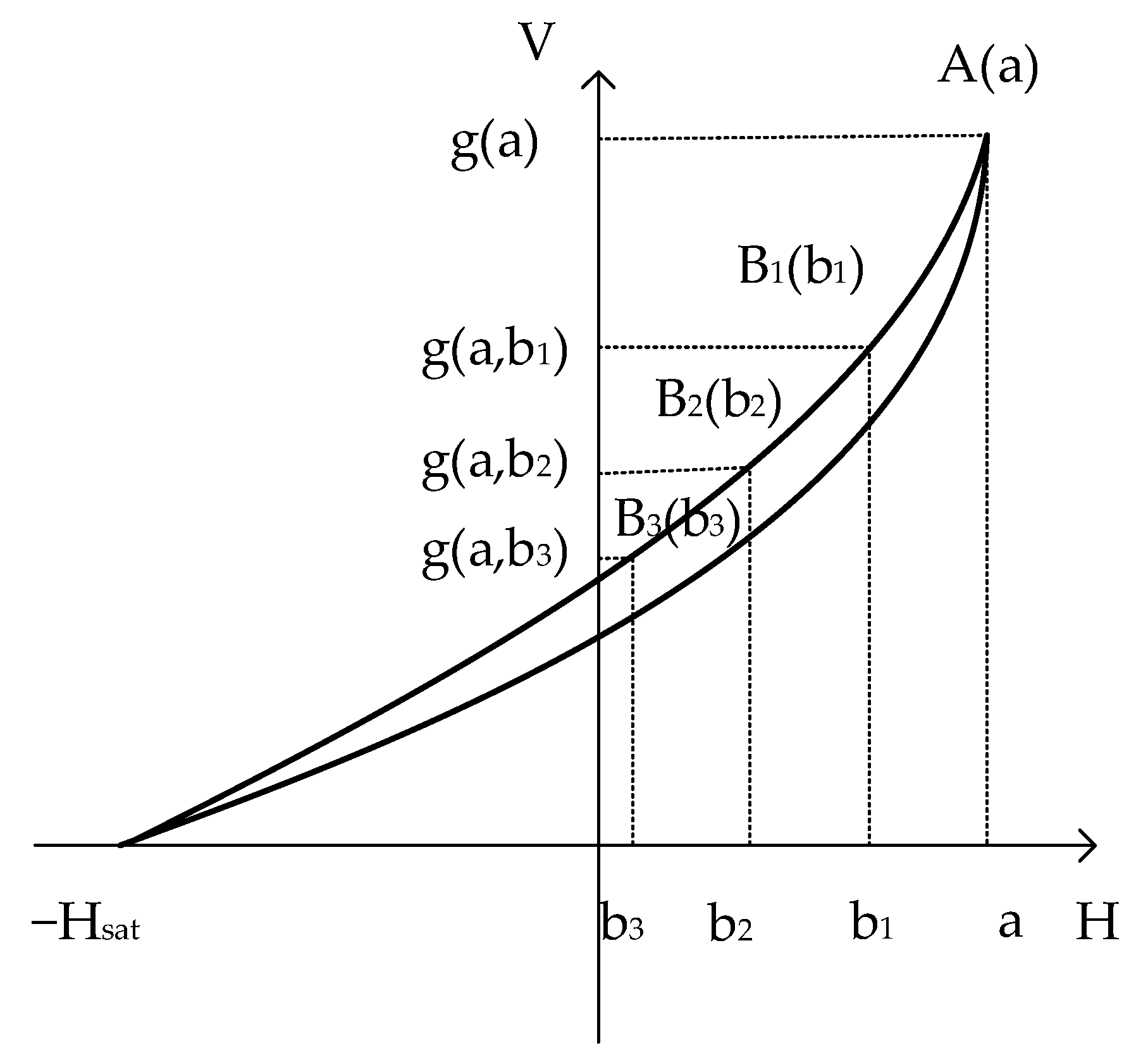
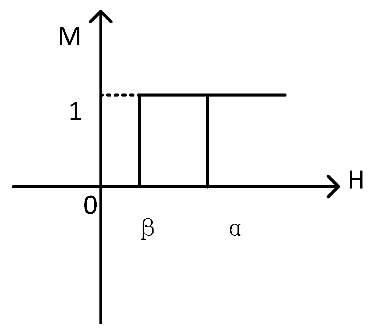
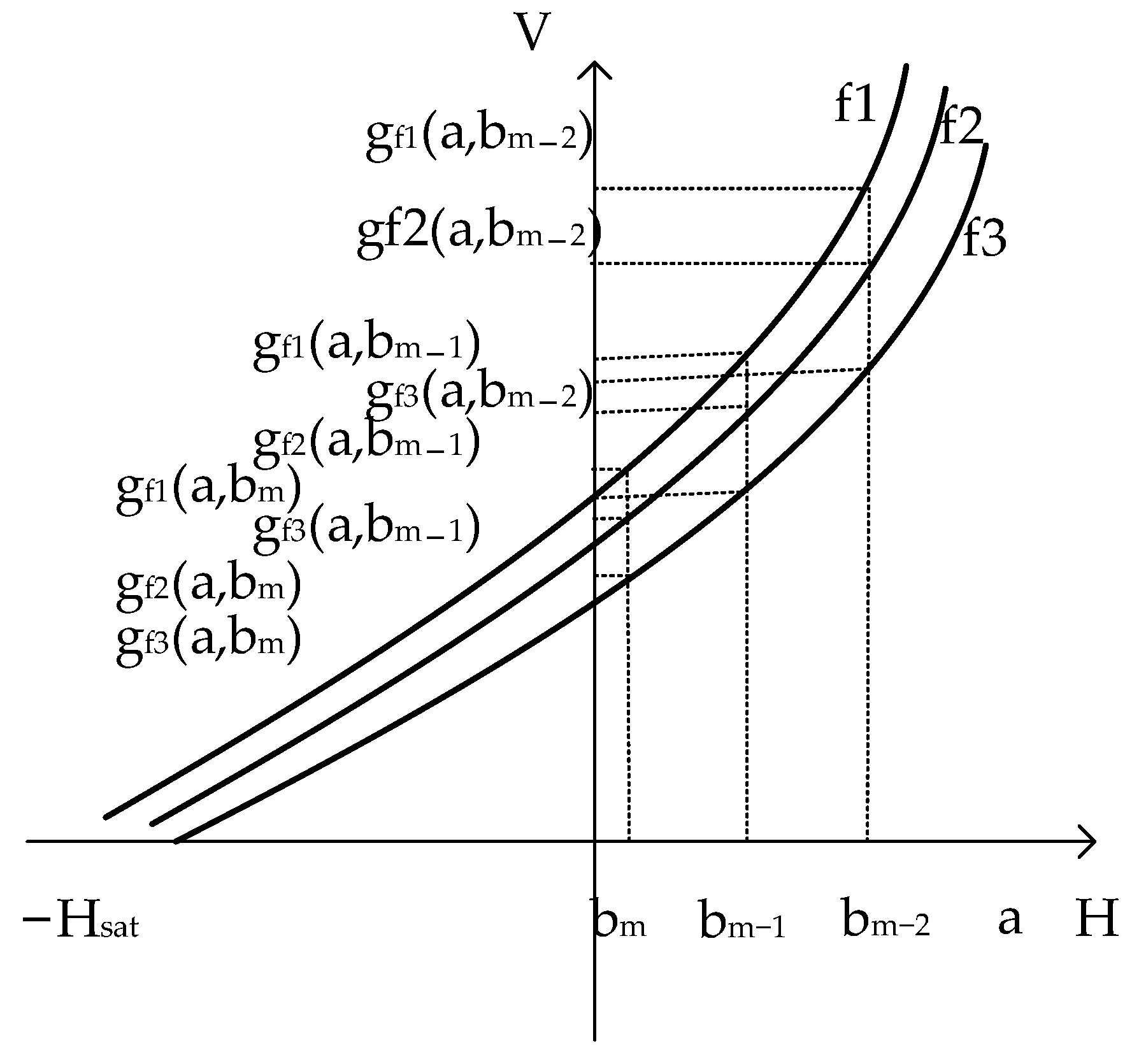
3.1. The Brief Introduction of the Static Model

This part briefly introduces the quasi-static hysteresis model based on probability, and the details can be found in reference [22]. The magnetoresistive element is regarded as a finite number of hysteresis operators. The graph of the hysteresis operator is shown in Figure 1.

In the figure, the H-axis is the strength of the applied magnetic field, and the M-axis is the value of the hysteresis operator, with only two values of 0 and 1. If the initial value of the hysteresis operator is 0 and the applied magnetic field gradually increases to be greater than or equal to α, then the value of the hysteresis operator becomes 1. Suppose that the initial value of the hysteresis operator is 1 and the applied magnetic field gradually decreases to less than or equal to β; the value of the hysteresis operator becomes 0. The expression is shown in Equation (1):

$${\mathsf{\gamma }\prime }_{\mathsf{\alpha }\mathsf{\beta }}=\{\begin{array}{ll}1& \mathrm{H}\ge \mathrm{a}\\ \mathrm{Nochange}& \mathrm{Others}\\ 0& \mathrm{H}\le \mathrm{b}\end{array}$$

(1)

where γ’ represents the hysteresis operator, and H is the strength of the applied magnetic field. The output of the magneto resistive sensor can be expressed as follows:

$$\mathrm{f}\left(\mathrm{u}\right(\mathrm{t}\left)\right)={{\displaystyle \iint }}_{\mathsf{\beta }\le \mathsf{\alpha }}^{}\mathrm{u}\left(\mathsf{\alpha },\mathsf{\beta }\right){\mathsf{\gamma }\prime }_{\mathsf{\alpha }\mathsf{\beta }}\mathrm{U}\left(\mathrm{t}\right)d\mathsf{\alpha }d\mathsf{\beta }$$

(2)

where $\mathrm{u}\left(\mathsf{\alpha },\mathsf{\beta }\right)$ is the weight function, γ’ is the hysteresis operator, U(t) is the input, and f(u(t)) is the output of the sensor. Since the value of the hysteresis operator is only 0 and 1, the hysteresis operator with the value of 0 can be ignored during integration, and only the hysteresis operator with the value of 1 can be integrated. This is equivalent to the number of hysteresis operators with the value of 1. Accordingly, when the intensity of the applied magnetic field is greater than or equal to the positive saturated magnetic field, the value of all hysteresis operators is 1. Divide the output of the sensor by that at positive saturation to obtain the proportion of the hysteresis operator with value 1. This is also the probability of the hysteresis operator satisfying this condition. Moreover, the probabilistic sensor output is as follows:

$$\mathrm{g}\left(\mathrm{t}\right)=\frac{f\left(\mathrm{u}\right(\mathrm{t}\left)\right)}{f\left(+\mathrm{Hsat}\right)}$$

(3)

where f(u(t)) is the output of the sensor under input u(t), f(+Hsat) represents the output of the sensor under the positive saturated magnetic field, and g(T) is the probabilistic sensor output.

Let A(a) and B(b) represent the random variables of the upper and lower threshold of the hysteresis operator, respectively. P(A) and P(B), respectively, represent the probability that the upper threshold of the hysteresis operator is less than a and the lower threshold is less than B. It has the following formula:

$$\mathrm{P}\left(\mathrm{A}=\mathrm{a}\right)={\mathrm{g}}^{+}\left(\mathrm{a}\right)$$

(4)

$$\mathrm{P}\left(\mathrm{B}=\mathrm{b}\right)={\mathrm{g}}^{-}\left(\mathrm{b}\right)$$

(5)

where ${\mathrm{g}}^{+}\left(\mathrm{a}\right)$ and ${\mathrm{g}}^{-}\left(\mathrm{b}\right)$ are the limit rising curve and limit falling curve, respectively [22,40].

The model satisfies the wipe-out property and the equal vertical chords property. The wipe-out property is that the model will preserve the influence of the input extreme value. Still, the new extreme value will eliminate the impact of the old extreme value, for which its absolute value is smaller than the new extreme value [22].

The equal vertical chords constitute all minor loops resulting from back-and-forth input variations between the same two consecutive extrema possessing equal vertical chords (output increments) for the same input values [22].

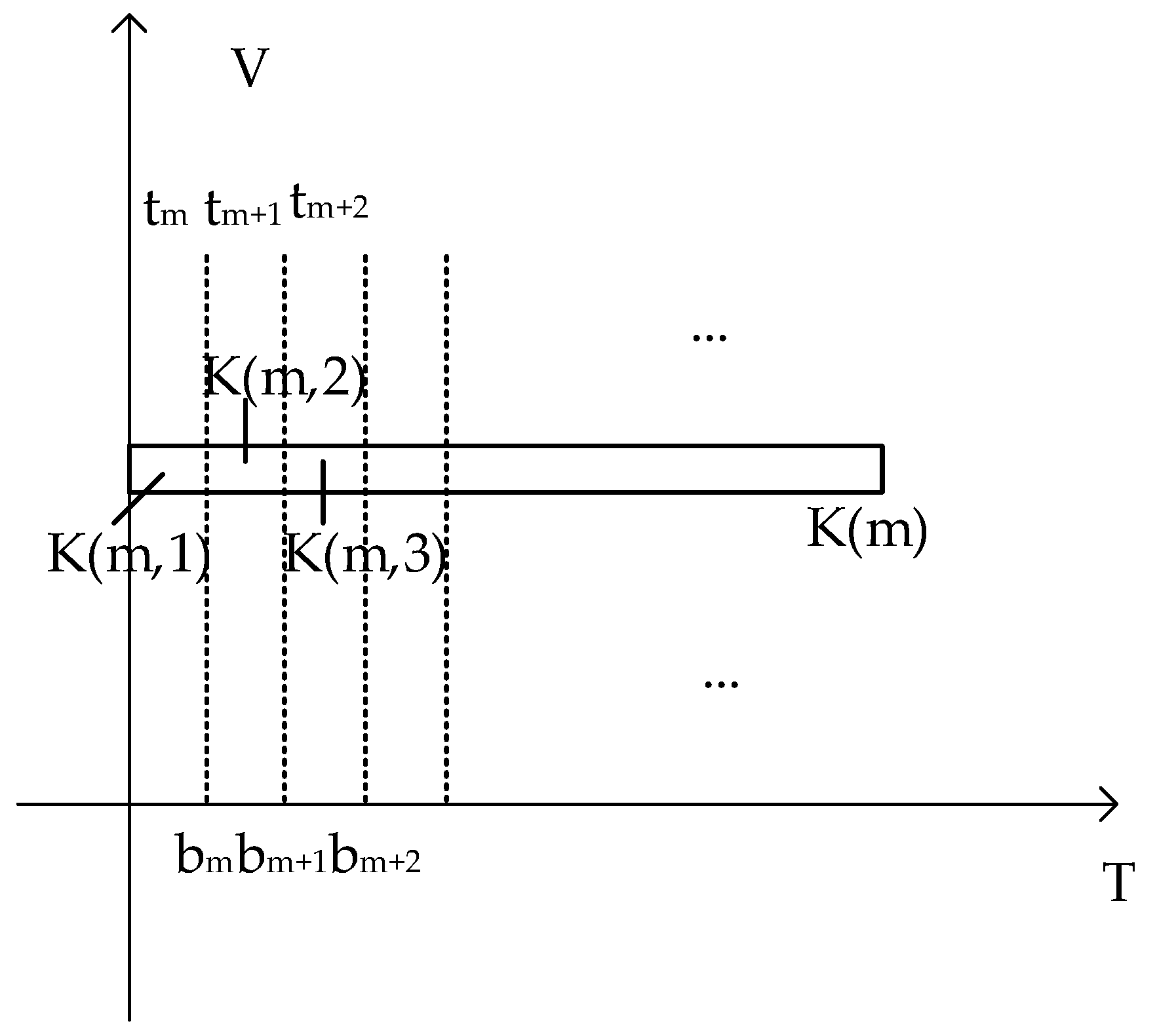
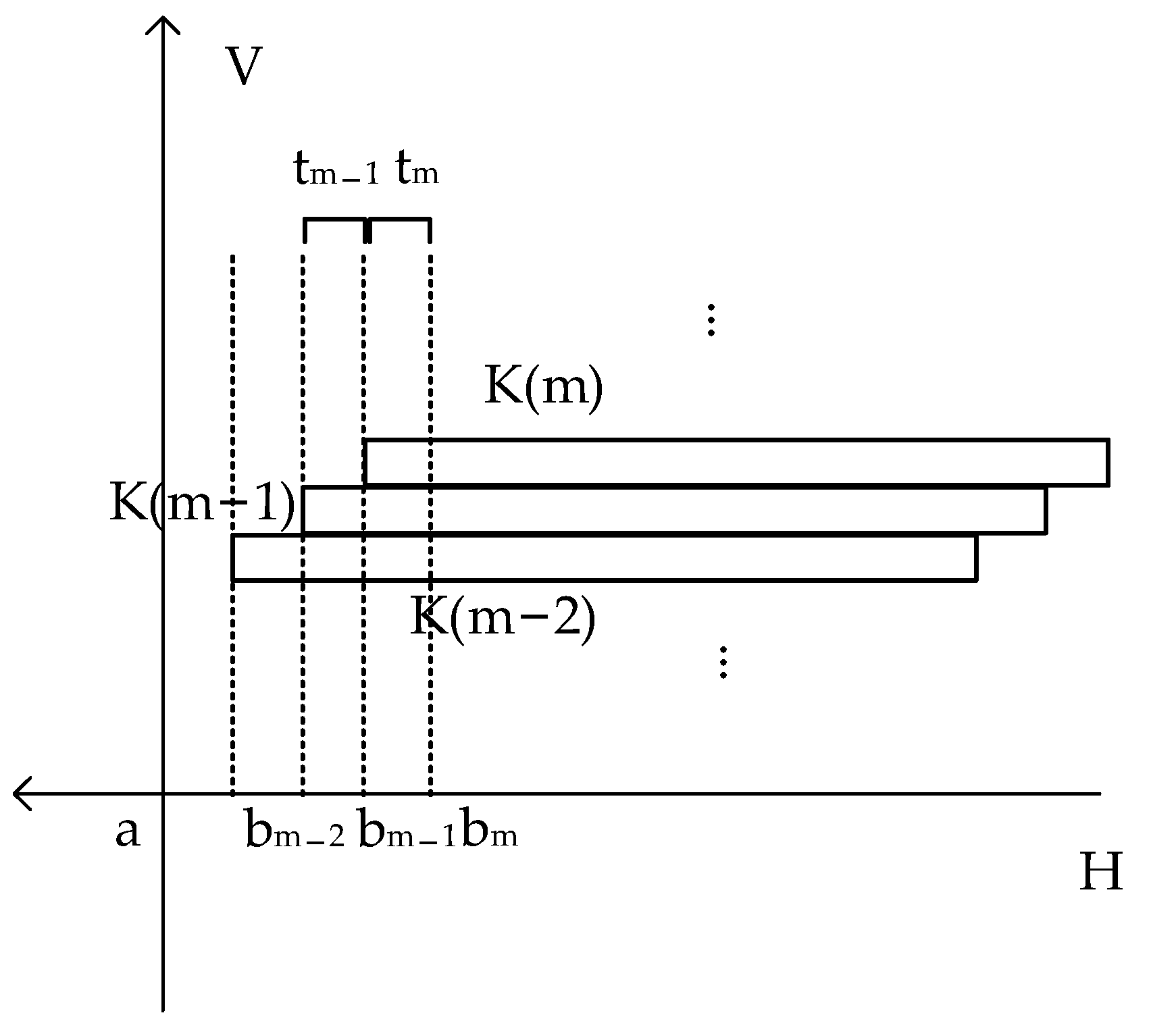
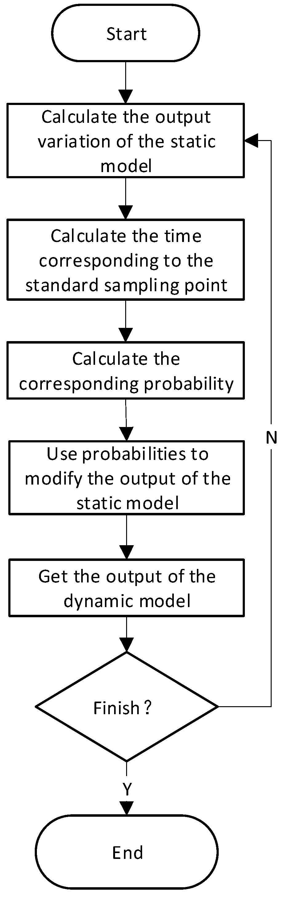
3.2. Introduction to Dynamic Hysteresis Model

The probability-based dynamic hysteresis model is constructed by introducing time-dependent random variables based on the static hysteresis model. Without losing generality, we will discuss the first-order rotation curve. As shown in Figure 2.

In the figure, A(a) is the turning point, and B₁(b₁), B₂(b₂), and B₃(b₃) are a series of equidistant points on the first-order rotation curve called standard sampling points; g(a, b₁), g(a, b₂), and g(a, b₃) are the corresponding outputs. When this curve is a static (quasi-static) curve, g(A, B_m) represents the probability that the upper threshold of the hysteresis operators is less than a, and the lower threshold is less than b_m. Then, K_m = g(A, B_m) − g(A, B_m−1) represents the probability of the operators for which their upper thresholds are less than a and the lower threshold is between b_m and b_m−1.

When the frequency is high, the first-order descending curve of different frequencies is shown in Figure 3.

In the figure, b_m, b_m−1, and b_m−2 are different inputs, while the three curves are the first-order descent curves at three different frequencies, f₁, f₂, and f₃, and g_fn(a,b_m) is the corresponding output of the sensor at different frequencies. It can be seen that the amount of change between the same input B_m−1 and B_m is different. This is due to the conversion speed of the operator is inconsistent, so it is necessary to introduce time-dependent variables. The hysteresis operator in which its upper threshold is less than or equal to a is recorded, and the lower threshold is between b_m−1 and b_m as in K(m). The time distribution of the hysteresis operator at a specific frequency is shown in Figure 4.

In the figure, a represents the rotation point of the first-order curve. b_m−2, b_m−1, and b_m represents the point on the first-order curve. t_m−1 represents the time when b_m−2 reaches b_m−1, and t_m represents the time when b_m−1 obtains b_m. K(m−1) means the hysteresis operators with the upper threshold less than or equal to a, and the lower threshold is between b_m−2 and b_m−1. K(m) represents the hysteresis operator with the upper threshold less than or equal to a and the lower threshold between b_m−1 and b_m. There are many similar hysteresis operators in addition to the drawn hysteresis operators. The left side of K(m) in the figure represents the threshold condition; that is, after the input meets the threshold condition, the value of this hysteresis operator begins to change. The length of K(m) represents the time required for all hysteresis operators contained in K(m) to complete the conversion. The graph of K(m) is shown in Figure 5.

In the figure, K(m) is the set of the hysteresis operators of segment m, t_m is the time from b_m−1 to b_m. K(m,1) is the hysteresis operator that completes the conversion in the first time segment of the hysteresis operator K(m). K(m,2) is the hysteresis operator that completes the conversion in the second time segment of K(m). K(m,3) is the hysteresis operator that completes the conversion in the third time segment of K(m) and so on.

At this frequency, the change M_m of the first-order rotation curve from b_m−1 to b_m is the sum of the hysteresis operators in this period from K(1) to K(m) in Figure 4. It can be expressed as Equation (6):

M_m = g’(A, B_m) − g’(A, B_m−1)

(6)

where g’ represents the probability at high frequency, and M_m is the variable from B_m−1 to B_m. Let f represent the frequency, m represents the coding of the variation, and n rep-resents the nth time stage after meeting the conditions of the variation m. Then, K_f(m,n) represents the number of the hysteresis operator in variation m with the conversion time in the nth time stage. Then, at high frequencies, any variation M_f,m can be expressed as follows.

M_f,m = K_f(m,1) + K_f(m−1,2) + K_f(m−2,3) + …

(7)

If we can find the items on the right, the problem can be solved. However, it is almost impossible to solve the problem due to too many variables. Therefore, the issue needs to be simplified. In order to simplify processing, the following conditions are set. Firstly, time t between the points is assumed to be the same. Since the distance between the points has been considered the same, the input slope between the points is the same. This means that the input waveform is a triangular wave. Secondly, it is assumed that the operators complete conversions within 2 t. Then, the following is obtained.

M_f,m = K_f(m,1) + K_f(m−1,2)

(8)

M_f/2,m = K_f(m,1) + K_f(m,2)

(9)

Therefore, all frequencies can be set to adopt frequency doubling, with a minimum of 1 Hz. Here, the lowest frequency 1 Hz can be regarded as quasi-static. According to the conditions set above, let s represent the order of frequency; then, we have the following.

f_s = 2f_s−1

(10)

For a particular point B_m on a specific frequency s, we have the following.

M_s,m = K_s(m,1) + Ks(m−1,2)

(11)

M_s−1,m = K_s(m,1) + K_s(m,2)

(12)

When s = 1, i.e., the frequency is 1 Hz, it is regarded as quasi-static.

M_1,m = g₁(A,B_m) − g₁(A,B_m−1)

(13)

When s = 2, i.e., the frequency is 2 Hz for B1, and its variation should contain two parts: the down-stage and up-stage. The down-stage is the stage in which the input decreases from A to B₁. It contains the operators with lower thresholds between B₁ and A for which the conversion time is less than t. The up-stage is the stage where the input increases from B₁ to A. It has operators with upper thresholds between B1 and A for which the conversion time is between t and 2 t. However, the current input does not meet the up-stage threshold conditions anymore, so it is considered 0.

M_2,1 = K₂(1,1)

(14)

According to Equation (12), we have the following.

M_1,1 = K₂(1,1) + K₂(1,2)

(15)

Then, we have the following.

K₂(1,2) = M_1,1 − M_2,1

(16)

For B2, there is the following equation.

M_2,2 = K₂(2,1) + K₂(1,2)

(17)

M_1,2 = K₂(2,1) + K₂(2,2)

(18)

The following is obtained.

K₂(2,1) = M_2,2 − K₂(1,2)= M_2,2 − (M_1,1 − M_2,1)

(19)

$${\mathrm{K}}_2\left(2,2\right)={\mathrm{M}}_{1,2}-{\mathrm{K}}_2\left(2,1\right)={\mathrm{M}}_{1,2}-{\mathrm{M}}_{2,2}+\left({\mathrm{M}}_{1,1}-{\mathrm{M}}_{2,1}\right)={{\displaystyle \sum }}_{\mathrm{p}=1}^2({\mathrm{M}}_{1,\mathrm{p}}-{\mathrm{M}}_{2,\mathrm{p}})$$

(20)

Similarly, for B3, we have the following.

$${\mathrm{K}}_2\left(3,1\right)={\mathrm{M}}_{2,3}-{\mathrm{K}}_2\left(2,2\right)={\mathrm{M}}_{2,3}-{{\displaystyle \sum }}_{\mathrm{p}=1}^2\left(({\mathrm{M}}_{1,\mathrm{p}}-{\mathrm{M}}_{2,\mathrm{p}}\right)$$

(21)

$${\mathrm{K}}_2\left(3,2\right)={\mathrm{M}}_{1,3}-{\mathrm{K}}_2\left(3,1\right)={\mathrm{M}}_{1,3}-{\mathrm{M}}_{2,3}+{{\displaystyle \sum }}_{\mathrm{p}=1}^2\left({\mathrm{M}}_{1,\mathrm{p}}-{\mathrm{M}}_{2,\mathrm{p}}\right)={{\displaystyle \sum }}_{\mathrm{p}=1}^3({\mathrm{M}}_{1,\mathrm{p}}-{\mathrm{M}}_{2,\mathrm{p}})$$

(22)

Suppose at some point Bn−1, the following is satisfied.

$${\mathrm{K}}_2\left(\mathrm{m}-1,1\right)={\mathrm{M}}_{2,\mathrm{m}-1}-{{\displaystyle \sum }}_{\mathrm{p}=1}^{\mathrm{m}-2}({\mathrm{M}}_{1,\mathrm{p}}-{\mathrm{M}}_{2,\mathrm{p}})$$

(23)

$${\mathrm{K}}_2\left(\mathrm{m}-1,2\right)={{\displaystyle \sum }}_{\mathrm{p}=1}^{\mathrm{m}-1}({\mathrm{M}}_{1,\mathrm{p}}-{\mathrm{M}}_{2,\mathrm{p}})$$

(24)

Then, for B_m, we have the following.

$${\mathrm{K}}_2\left(\mathrm{m},1\right)={\mathrm{M}}_{2,\mathrm{m}}-{\mathrm{K}}_2\left(\mathrm{m}-1,2\right)={\mathrm{M}}_{2,\mathrm{m}}-{{\displaystyle \sum }}_{\mathrm{p}=1}^{\mathrm{m}-1}({\mathrm{M}}_{1,\mathrm{p}}-{\mathrm{M}}_{2,\mathrm{p}})$$

(25)

$${\mathrm{K}}_2\left(\mathrm{m},2\right)={\mathrm{M}}_{1,\mathrm{m}}-{\mathrm{K}}_2\left(\mathrm{m},1\right)={\mathrm{M}}_{1,\mathrm{m}}-{\mathrm{M}}_{2,\mathrm{m}}+{{\displaystyle \sum }}_{\mathrm{p}=1}^{\mathrm{m}-1}({\mathrm{M}}_{1,\mathrm{p}}-{\mathrm{M}}_{2,\mathrm{p}})={{\displaystyle \sum }}_{\mathrm{p}=1}^{\mathrm{m}}({\mathrm{M}}_{1,\mathrm{p}}-{\mathrm{M}}_{2,\mathrm{p}})$$

(26)

By analogy, all parameters of frequency 2 can be obtained.

Suppose that, for a certain frequency s−1, parameters K_s−1(m,1) and K_s−1(m,2) of any point B_m satisfy the following.

$${\mathrm{K}}_{\mathrm{s}-1}\left(\mathrm{m},1\right)={\mathrm{M}}_{\mathrm{s}-1,\mathrm{m}}-{{\displaystyle \sum }}_{\mathrm{p}=1}^{\mathrm{m}-1}({\mathrm{M}}_{1,\mathrm{p}}-{\mathrm{M}}_{2,\mathrm{p}})$$

(27)

$${\mathrm{K}}_{\mathrm{s}-1}\left(\mathrm{m},2\right)={{\displaystyle \sum }}_{\mathrm{p}=1}^{\mathrm{m}}({\mathrm{M}}_{1,\mathrm{p}}-{\mathrm{M}}_{2,\mathrm{p}})$$

(28)

Then, when calculating frequency s, and these equations are halved.

$${\mathrm{M}}_{\mathrm{s},1}={\mathrm{K}}_{\mathrm{s}}\left(1,1\right)$$

(29)

$${\mathrm{M}}_{\mathrm{s}-1,1}={\mathrm{K}}_{\mathrm{s}}\left(1,1\right)+{\mathrm{K}}_{\mathrm{s}}\left(1,2\right)$$

(30)

$${\mathrm{M}}_{\mathrm{s},2}={\mathrm{K}}_{\mathrm{s}}\left(2,1\right)+{\mathrm{K}}_{\mathrm{s}}\left(1,2\right)$$

(31)

$${\mathrm{M}}_{\mathrm{s}-1,2}={\mathrm{K}}_{\mathrm{s}}\left(2,1\right)+{\mathrm{K}}_{\mathrm{s}}\left(2,2\right)$$

(32)

We can obtain parameters K_s(m,1) and K_s(m,2) of each point B_m with the following equations.

$${\mathrm{K}}_{\mathrm{s}}\left(1,1\right)={\mathrm{M}}_{\mathrm{s},1}$$

(33)

$${\mathrm{K}}_{\mathrm{s}}\left(1,2\right)={\mathrm{M}}_{\mathrm{s}-1,1}-{\mathrm{M}}_{\mathrm{s},1}$$

(34)

$${\mathrm{K}}_{\mathrm{s}}\left(2,1\right)={\mathrm{M}}_{\mathrm{s},2}-\left({\mathrm{M}}_{\mathrm{s}-1,1}-{\mathrm{M}}_{\mathrm{s},1}\right)$$

(35)

$${\mathrm{K}}_{\mathrm{s}}\left(2,2\right)={{\displaystyle \sum }}_{\mathrm{p}=1}^2({\mathrm{M}}_{\mathrm{s}-1,\mathrm{p}}-{\mathrm{M}}_{\mathrm{s},\mathrm{p}})$$

(36)

Then, according to previous reasoning, the relevant parameters of any point B_m on frequency S can be calculated as follows.

$${\mathrm{K}}_{\mathrm{s}}\left(\mathrm{m},1\right)={\mathrm{M}}_{\mathrm{s},\mathrm{m}}-{{\displaystyle \sum }}_{\mathrm{p}=1}^{\mathrm{m}}({\mathrm{M}}_{1,\mathrm{p}}-{\mathrm{M}}_{2,\mathrm{p}})$$

(37)

$${\mathrm{K}}_{\mathrm{s}}\left(\mathrm{m},2\right)={{\displaystyle \sum }}_{\mathrm{p}=1}^{\mathrm{m}}({\mathrm{M}}_{1,\mathrm{p}}-{\mathrm{M}}_{2,\mathrm{p}})$$

(38)

Arrang K_s (m,1) corresponding to M_m in time. Calculate the ratio of K_s(m,1) to the change of the corresponding static model K₁(m,1). Then the time probability distribution of the hysteresis operator corresponding to the lower threshold between B_m−1 and B_m can be obtained. According to the static hysteresis model and this probability distribution, the different outputs corresponding to the inputs of different rates can be calculated to complete hysteresis modeling.

Because the accumulation method will cause the accumulation of errors, it is necessary to correct the data. In this paper, the outputs of the equal extreme value of each cycle should be equal and it is used to correct the data.

4. Experiment

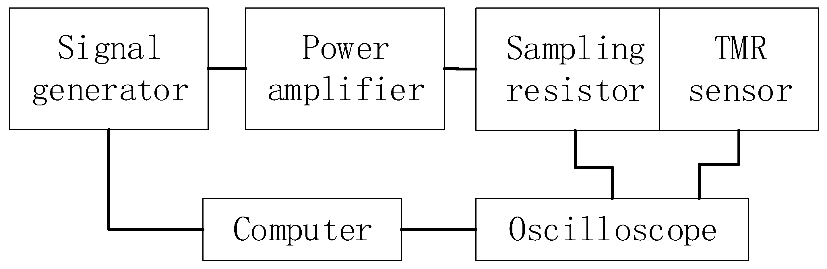
4.1. Experimental Structure

In order to eliminate the interference of the magnetic field generator, this paper adopts the method of electrifying straight wires to generate a magnetic field. This method has the best high-frequency performance and the best consistency between magnetic fields and currents. However, the magnetic field generated in this manner is relatively small, so we use a power amplifier. The generated magnetic field can basically reach the saturation region of the sensor. The problem of an uneven magnetic field caused by this magnetic field can also be avoided by using the method of tightly fixing the sensor plate.

The experiment adopts the structure shown in Figure 6. The triangular wave signal is generated by the signal generator Agilent 33250 A. Moreover, it is amplified by the power amplifier Matasusada DOS60-5. A sampling resistance was connected to the power amplifier by a straight wire. An oscilloscope Fluke MDO3054 measures the output of resistance. The sensor measures the magnetic field of the straight wire. The computer is used to control the entire acquisition process.

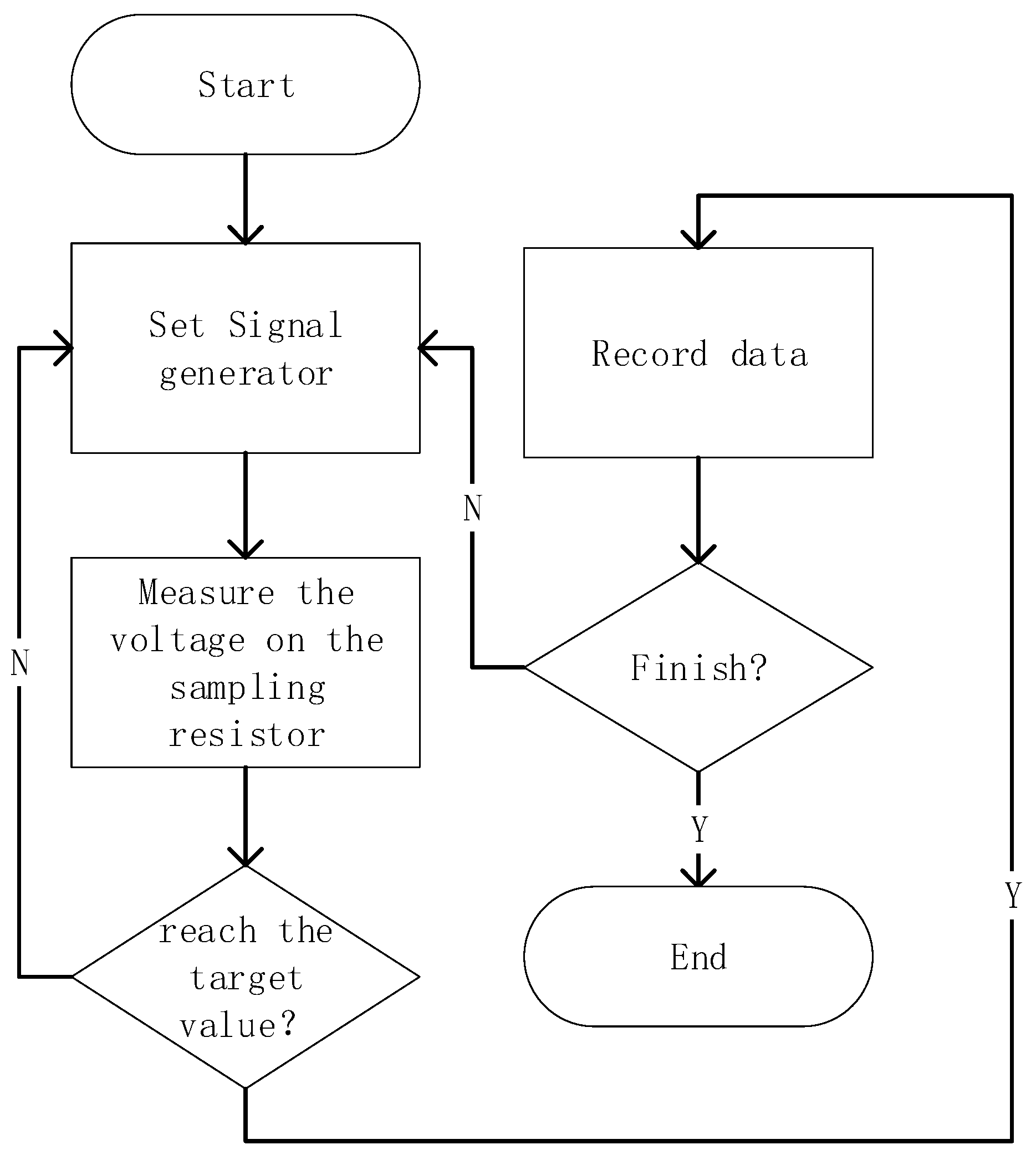
4.2. Experimental Process

The sampling flow chart is shown in Figure 7. First, the output target waveform of the signal generator is set. Then, the voltage on the sampling resistance is collected with an oscilloscope and we evaluate whether it meets the required value. If not, the output of the signal generator is adjusted until the required voltage value is reached. Otherwise, the voltage waveform of the sampling resistance and the output waveform of the sensor are collected.Then process the next point until all points for this frequency are processed.. Then, we proceed to the subsequent frequency until all frequencies are completed. Due to the performance limitation of the power amplifier, when the frequency reaches 16,384 Hz, the waveform is distorted and is no longer a triangular wave. Thus, 8192 Hz is the maximum frequency.

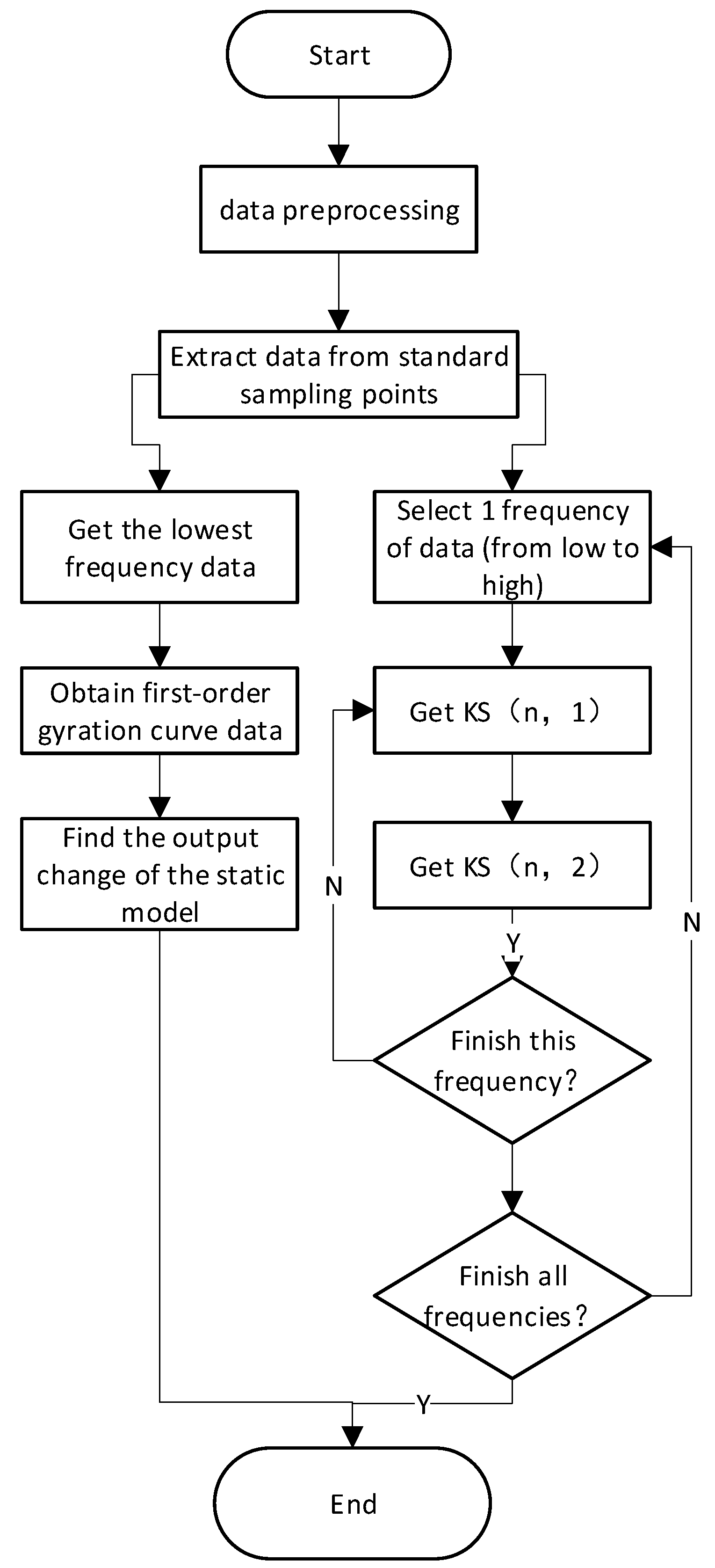
4.3. Data Processing

Data processing mainly processes the collected results to obtain the K_s value of each frequency, and the results are arranged according to time. The flow chart is shown in Figure 8. Firstly, the measured data are preprocessed. Preprocessing is the average processing of multi-cycle data. Then, the values of standard sampling points are extracted. The next step is divided into two parts. One is obtaining the static model using the lowest frequency data. The other is obtaining K_s(m,1). First, K₁(m,1) was calculated. Second, K₂(m,1) and K₂(m,2) are calculated. Then, the subsequent frequency is calculated until the data of all frequencies are processed. Then, all Ks(m,1) are arranged according to time, input, and rotation point. The probability distribution of conversion times can be obtained by parabolizing Ks(m,1) relative to the change of the static model at each standard sampling point.

When estimating the output, the flow chart is shown in Figure 9. Firstly, the output variation of the static model is calculated according to the input. Then, according to the slope of the input data, the corresponding time of the standard sampling point is calculated. The probability is obtained according to the rotation point, standard sampling point, and time corresponding to the standard sampling point. Finally, the probability is used to modify the output variation of the static model; then, the output of the dynamic model was obtained.

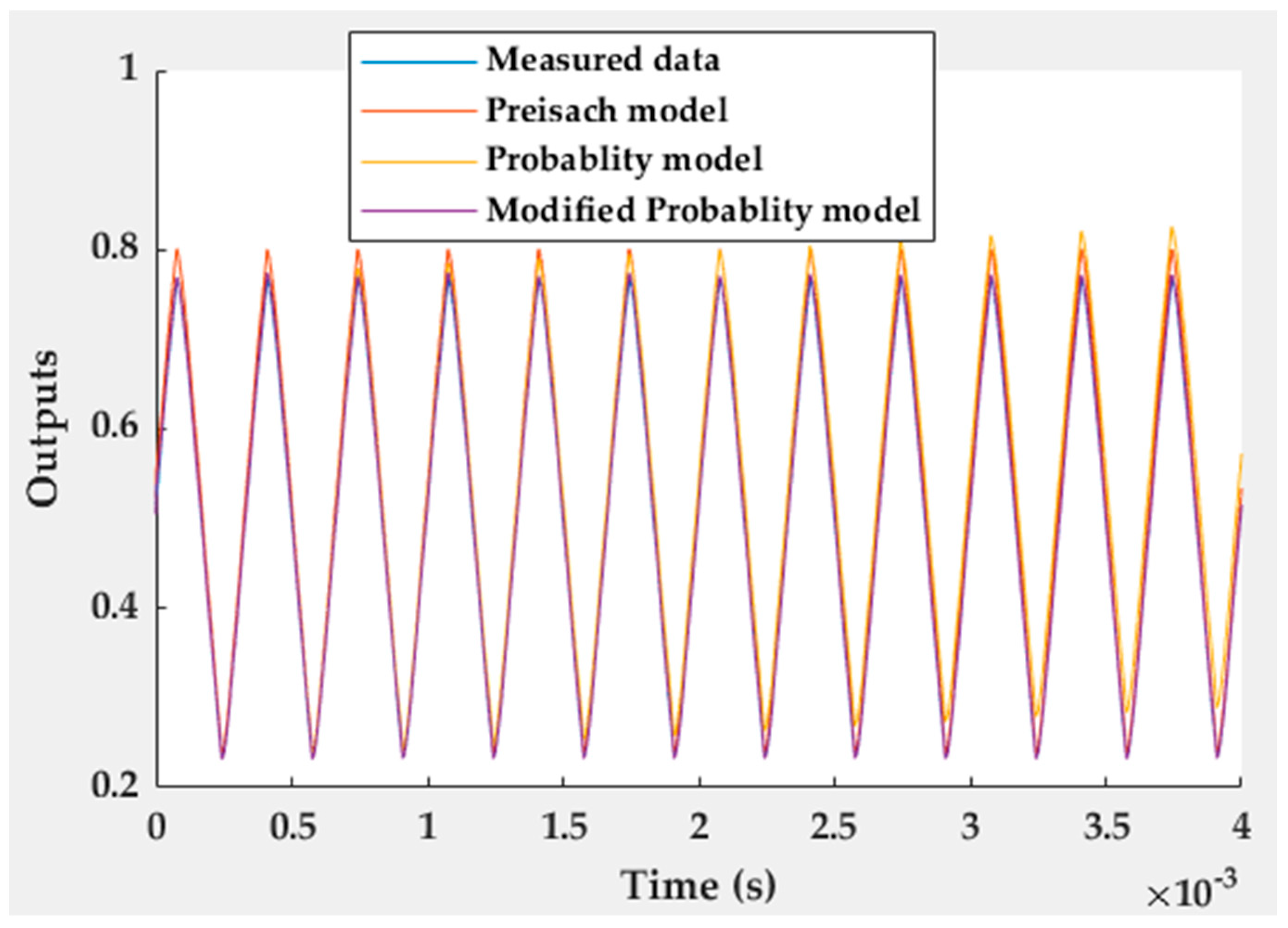
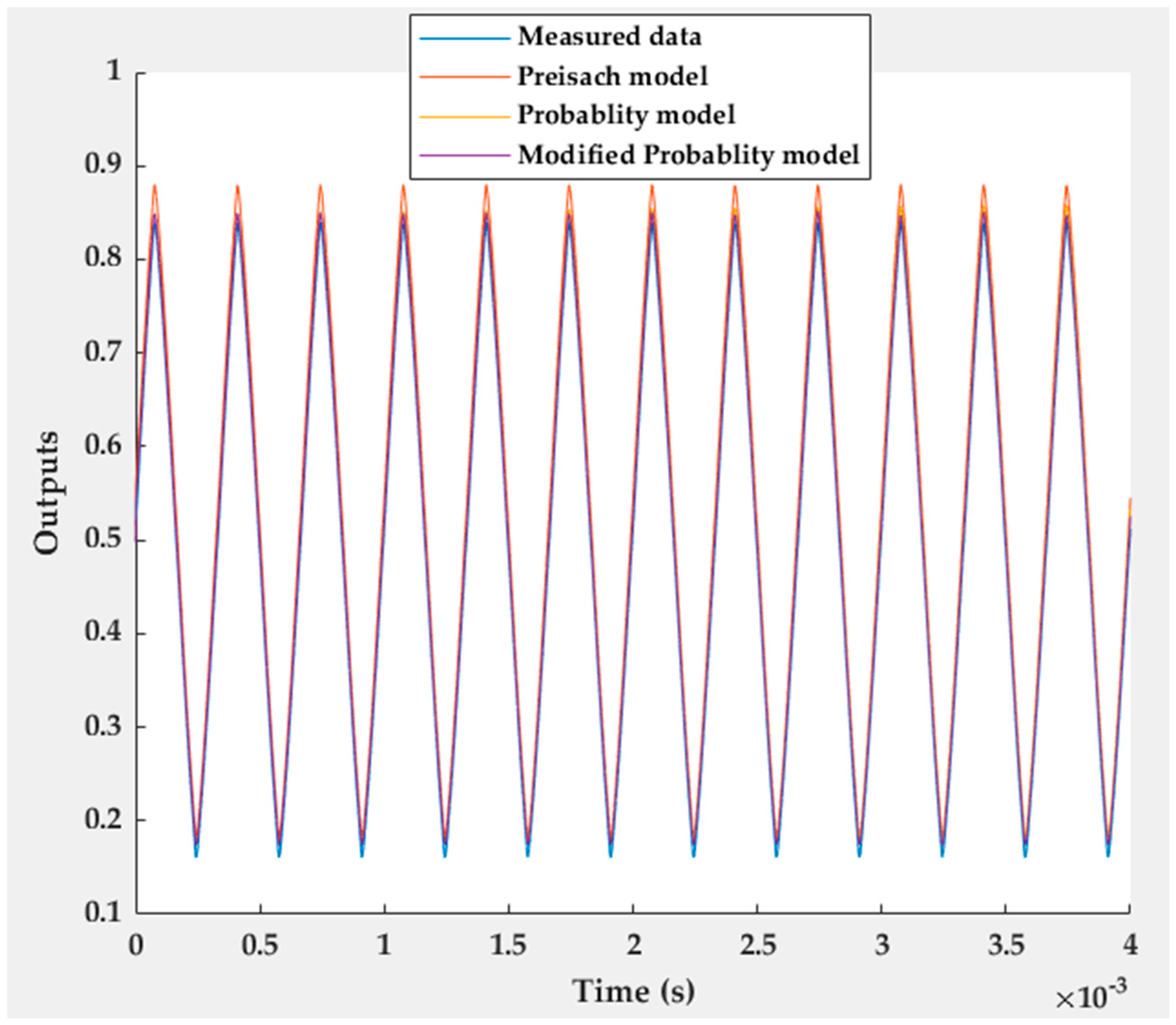
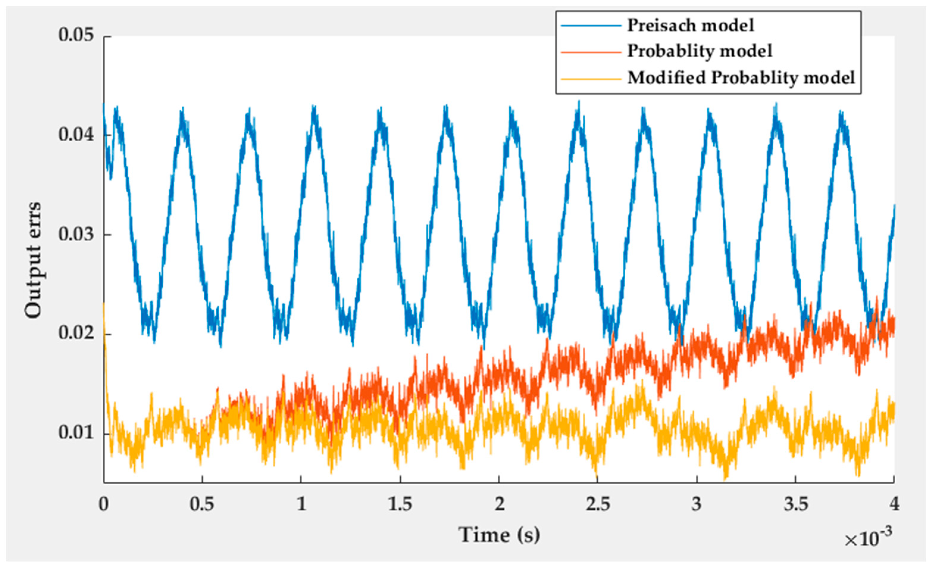
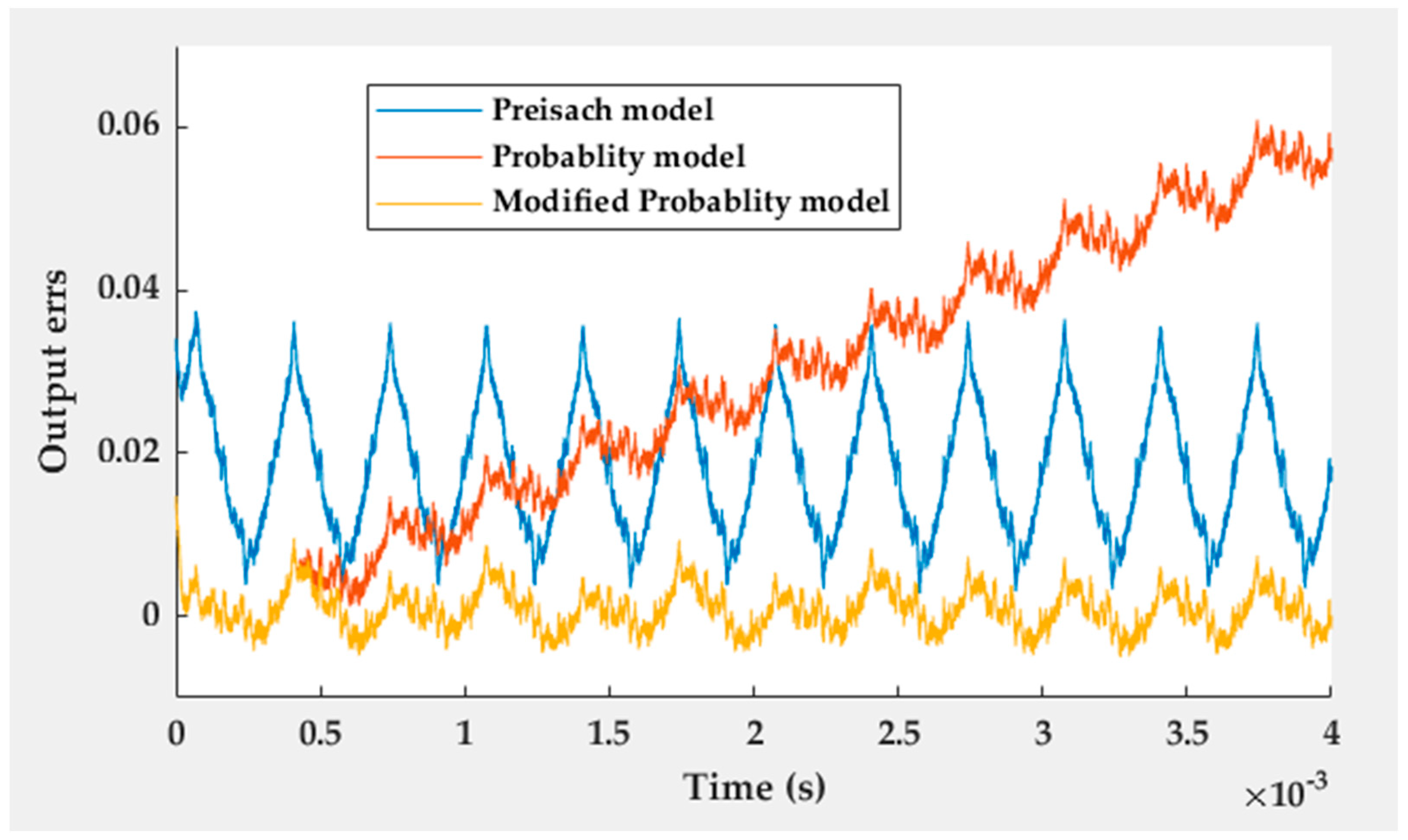
5. Results and Analysis

We use two sensors to verify the proposed method. The results of 3 kHz are shown in Figure 10 and Figure 11.

In the figures, the X-axis denotes time, and the Y-axis denotes the probabilistic output of the sensor. The blue curve represents the measured data. The red curve represents the data of the Preisach model. The yellow curve represents the data of the probability model. The purple curve represents the data of the modified probability model. It can be observed that the probability model is closer to the measured data compared to the Preisach model. However, the data of the uncorrected probability model will gradually deviate. The corrected probability model data will remain stable. This proves the effectiveness of the method. The errors of the results are shown in Figure 12 and Figure 13, respectively.

In the figures, blue is the error of the Preisach model, red is the error of the probability model, and yellow is the error of the modified probability model. It can be observed that the error of the probability model is much smaller than that of the Preisach model. Still, the error caused by accumulation induces a linear shift in the results of the probability model. The modified model solves this problem well. The error data of the two sensors are shown in

Table 2. The errors at 3 kHz.

		Maximum	Variance	Average Value
Sensor 1	Preisach model	0.0375	6.8488 × 10−5	0.0184
	Modified probability model	0.0147	6.6941 × 10−6	8.4390 × 10−4
	Improvement effect	60.8%	90.2%	95.4%
Sensor 2	Preisach model	0.0436	5.3854 × 10−5	0.0301
	Modified probability model	0.0232	2.7935 × 10−6	0.0105
	Improvement effect	46.7%	94.8%	65.1%

.

It can be obesrved that, for sensor 1, the maximum error of the Preisach model is 0.0375, the variance of the error is 6.8488 × 10⁻⁵, and the average value is 0.0184. The maximum error of the modified probability model is 0.0147, the variance is 6.6941 × 10⁻⁶, and the average value is 8.4390 × 10⁻⁴. Compared with the Preisach model, the maximum error of the probability model was reduced by 60.8%, the variance was reduced by 90.2%, and the average value was reduced by 95.4%. For sensor 2, the maximum error of the Preisach model is 0.0436, the error variance is 5.3854 × 10⁻⁵, and the average value is 0.0301. The maximum error of the modified probability model is 0.0232, the variance is 2.7935 × 10⁻⁶, and the average value is 0.0105. Compared with the Preisach model, the maximum error of the probability model is reduced by 46.7%, the variance is reduced by 94.8%, and the average value is reduced by 65.1%. We can see that the errors are greatly reduced especially the variances. This shows the effectiveness of the probability model. Moreover, the errors of 1 kHz and 5 kHz are shown in

Table 3. The errors at 1 kHz and 5 kHz.

Frequency	Metrics	Sensor 1			Sensor 2
		Preisach Model	Probability Model	Improve	Preisach Model	Probability Model	Improve
1 kHz	Maximum	0.0323	0.0134	58.5%	0.0205	0.006	70.7%
	Variance	6.49 × 10−5	1.44 × 10−5	77.8%	4.63 × 10−5	1.42 × 10−6	96.9%
	Average value	−0.0176	−0.0059	66.5%	−0.0095	0.0018	81.1%
5 kHz	Maximum	0.0296	0.0115	61.1%	0.0204	0.0066	67.6%
	Variance	6.38 × 10−5	7.99 × 10−5	87.5%	5.24 × 10−5	3.45 × 10−6	93.4%
	Average value	−0.0135	7.69 × 10−5	99.4%	−0.0088	0.0019	78.4%

.

In Table 3, at 1 kHz, the maximum error of the Preisach model is 0.0323 for sensor 1, the variance of the error is 6.49 × 10⁻⁵, and the average value is −0.0176. The maximum error of the modified probability model is 0.0134, the variance is 1.44 × 10⁻⁵, and the average value is −0.0059. Compared with the Preisach model, the maximum error of the probability model was reduced by 58.5%, variance was reduced by 77.8%, and the average value was reduced by 66.5%. For sensor 2, the maximum error of the Preisach model is 0.0205, the error variance is 4.63 × 10⁻⁵, and the average value is −0.0095. The maximum error of the modified probability model is 0.006, the variance is 1.42 × 10⁻⁶, and the average value is 0.0018. Compared with the Preisach model, the maximum error of the probability model was reduced by 70.7%, the variance was reduced by 96.9%, and the average value was reduced by 81.1%.

At 5 KHz, for sensor 1, the maximum error of the Preisach model is 0.0296, the variance of the error is 6.38 × 10⁻⁵, and the average value is −0.0135. The maximum error of the modified probability model is 0.0115, the variance is 7.99 × 10⁻⁶, and the average value is 7.69 × 10⁻⁵. Compared with the Preisach model, the maximum error of the probability model was reduced by 61.1%, variance was reduced by 87.5%, and the average value was reduced by 99.4%. For sensor 2, the maximum error of the Preisach model is 0.0204, the error variance is 5.24 × 10⁻⁵, and the average value is −0.0088. The maximum error of the modified probability model is 0.0066, the variance is 3.45 × 10⁻⁶, and the average value is 0.0019. Compared with the Preisach model, the maximum error of the probability model was reduced by 67.6%, variance was reduced by 93.4%, and the average value was reduced by 78.4%.

We can see that the errors are greatly reduced, especially the variances. This shows the effectiveness of the probability model.

6. Conclusions

Dynamic hysteresis is the primary research area affecting the accuracy of TMR sensors. However, there are varieties of related research, but it is still a research focus.

Based on the quasi-static probability model, this paper further regards the variation of the same input amplitude with different frequencies as the time distribution of the hysteresis operator. Then, the calculation method of the time distribution is deduced by adding some limiting conditions. Finally, the dynamic hysteresis model is constructed by using the static model and time distribution modeling. However, deviation propogation causes a shift in the results. Therefore, a cured method using the characteristic of equal periodic extremum output was proposed. Two sensors are used to verify the model at 1 kHz, 3 kHz, and 5 KHz, respectively. The results show that the maximum error can be reduced by 46.7%, the variance can be reduced by 77.8%, and the average value can be reduced by 65.1%. This shows that the model can effectively reduce errors caused by hysteresis and proves its effectiveness. The performance improvement of this model may be due to the following reasons. First, this model adopts a high-frequency triangular wave signal, while the Preisach model adopts a measuring step relaxation time constant. Second, the model can calculate more detailed time distributions, which helps reduce errors. In addition, this model mainly regards the sensor as a set of hysteresis operators and then calculates the probability and time distribution of hysteresis operators, which has little to do with the specific sensor type; therefore, it should have better generalization abilities. Interpolation is mainly used in the solution process after the model is established. The algorithm is relatively simple, and the calculation speed is swift. This model is relatively simple, easy to implement, and is irreversible. Still, suppose that the appropriate hysteresis operator is selected. In that case, it may also be used to model the inverse problem directly in order to solve the reversible problem, which will be the next attempt.

The innovations of this paper are as follows: (1) The dynamic hysteresis characteristics of TMR are studied and applied to dynamic measurements; (2) the time distribution characteristic is introduced into the static probabilistic hysteresis model, and the probabilistic model is applied to the dynamic hysteresis model; (3) compared with the Preisach model, the maximum error of this method can be reduced by 46.7%, the variance can be reduced by 77.8%, and the average value can be reduced by 65.1%.

References

1. Baibich, M.N.; Broto, J.M.; Fert, A.; Van Dau, F.N.; Petroff, F.; Etienne, P.; Creuzet, G.; Friederich, A.; Chazelas, J. Giant magnetoresistance of (001) Fe/(001) Cr magnetic superlattices. Phys. Rev. Lett. 1988, 61, 2472. [Google Scholar] [CrossRef] [PubMed] [Green Version]
2. Binasch, G.; Grünberg, P.; Saurenbach, F.; Zinn, W. Enhanced magnetoresistance in layered magnetic structures with antiferromagnetic interlayer exchange. Phys. Rev. B 1989, 39, 4828–4830. [Google Scholar] [CrossRef] [PubMed] [Green Version]
3. Neeraja, R.; Sarah, E.C.; Luis, M.F. A GMR-based assay for quantification of the human response to influenza. Biosens. Bioelectron. 2022, 205, 114086. [Google Scholar] [CrossRef]
4. Li, X.; Hu, J.; Chen, W.; Yin, L.; Liu, X. A Novel High-Precision Digital Tunneling Magnetic Resistance-Type Sensor for the Nanosatellites Space Application. Micromachines 2018, 9, 121. [Google Scholar] [CrossRef] [PubMed] [Green Version]
5. Yuan, X.; Li, W.; Chen, G.; Yin, X.; Ge, J. Uniform Current Field Testing System with TMR Sensor Array for Non-contact Detection and Estimation of Cracks on Power Plant Piping. Sens. Actuators A Phys. 2017, 263. [Google Scholar]
6. Masami, M.; Fumio, K.; Naoki, K. ESD tolerance of gmr and tmr heads within hard disk drive. IEEE Trans. Device Mater Reliab. 2010, 10, 476–481. [Google Scholar]
7. Patrick, N.A.; Qi, H.; Dongsheng, C.; Olusola, B.; Paul, O.K.A. Real-time and contactless initial current traveling wave measurement for overhead transmission line fault detection based on tunnel magnetoresistive sensors. Electr. Power Syst. Res. 2020, 187, 106508. [Google Scholar]
8. Daniel, K.; Kütt, L.; Iqbal, M.N.; Shabbir, N.; Rehman, A.U.; Shafiq, M.; Hamam, H. Current Harmonic Aggregation Cases for Contemporary Loads. Energies 2022, 15, 437. [Google Scholar] [CrossRef]
9. Wang, S.; Wu, Z.; Peng, D.; Li, W.; Chen, S.; Liu, S. An angle displacement sensor using a simple gear. Sens. Actuators A Phys. 2018, 270, 245–251. [Google Scholar] [CrossRef]
10. Knudde, S.; Farinha, G.; Leitao, D.; Ferreira, R.; Cardoso, S.; Freitas, P. AlOx barrier growth in magnetic tunnel junctions for sensor applications. J. Magn. Magn. Mater. 2016, 412, 181–184. [Google Scholar] [CrossRef]
11. Xiaodong, Z.; Zheng, Q. The influence on hysteresis from the ending pinning design of GMR free layer. Microsyst. Technol. 2016, 22, 137–141. [Google Scholar] [CrossRef]
12. John, M.A.; Arthur, V.P. Ultra-Low Hysteresis and Self-Biasing in GMR Sandwich Sensor Element. IEEE Trans. Magn. 2001, 37, 4. [Google Scholar]
13. Michal, V.; Pavel, R.; Jan, K.; Mark, T. Improved GMR sensor biasing design. Sens. Actuator A Phys. 2004, 110, 254–258. [Google Scholar]
14. Christian, B.; Roland, W. Correcting nonlinearity and temperature influence of sensors through B-Spline modeling. In Proceedings of the 2010 IEEE International Symposium on Industrial Electronics, Bari, Italy, 4–7 July 2010; pp. 3356–3361. [Google Scholar]
15. Jinchi, H.; Jun, H.; Yong, O.; Shan, W.; Jinliang, H. Hysteretic Modeling of Output Characteristics of Giant Magneto-Resistive Current Sensors. IEEE Trans. Ind. Electron. 2014, 9, 1–9. [Google Scholar]
16. Branko, K.; Alenka, M.; Nebojsa, M. Mathematical modelling of frequency-dependent hysteresis and energy loss of FeBSiC amorphous alloy. J. Magn. Magn. Mater. 2017, 422, 37–42. [Google Scholar]
17. Christian, G.; Marco, B.; Mariano, P.; Nicholas, S. Dynamic Ferromagnetic Hysteresis Modelling Using a Preisach-Recurrent Neural Network Model. Materials 2020, 13, 256. [Google Scholar]
18. Kucuk, I.; Derebasi, N. Dynamic hysteresis modelling for toroidal cores. Phys. B 2006, 372, 260–264. [Google Scholar] [CrossRef]
19. Yonghong, T.; Liang, D. Modeling the dynamic sandwich system with hysteresis using NARMAX model. Math. Comput. Simul. 2014, 97, 162–188. [Google Scholar]
20. Jiles, D.; Atherton, D. Ferromagnetic hysteresis. IEEE Trans. Magn. 1983, 19, 2183–2185. [Google Scholar] [CrossRef]
21. Krasnosel’skii, M.A.; Pokrovskii, A.V. Systems with Hysteresis; Springer: New York, NY, USA, 1989. [Google Scholar]
22. Yutao, L.; Liliang, W.; Hao, Y.; Zheng, Q. Research of Probability-Based Tunneling Magnetoresistive Sensor Static Hysteresis Model. Sensors 2021, 21, 7672. [Google Scholar] [CrossRef]
23. Negulescu, B.; Lacour, D.; Montaigne, F.; Gerken, A.; Paul, J.; Spetter, V.; Marien, J.; Duret, C.; Hehn, C. Wide range and tunable linear magnetic tunnel junction sensor using two exchange pinned electrodes. Appl. Phys. Lett. 2009, 95, 11. [Google Scholar] [CrossRef] [Green Version]
24. Ku, W.; Silva, F.; Bernardo, J.; Freitas, P.P. Integrated giant magnetoresistance bridge sensors with transverse permanent magnet biasing. J. Appl. Phys. 2000, 87, 5352–5355. [Google Scholar] [CrossRef]
25. Liao, S.-H.; Huang, H.-S.; Sokolov, A.; Yang, Y.; Liu, Y.-F.; Yin, X.; Wilson, A.; Trujilo, A.; Ewing, D.; Liou, S.-H. Hysteresis Reduction in Tunneling Magnetoresistive Sensor with AC Modulation Magnetic Field. IEEE Trans. Magn. 2021, 57, 1–4. [Google Scholar] [CrossRef]
26. Xie, F.; Weiss, R.; Weigel, R. Hysteresis Compensation Based on Controlled Current Pulses for Magnetoresistive Sensors. IEEE Trans. Ind. Electron. 2015, 62, 7804–7809. [Google Scholar] [CrossRef]
27. Grandi, G.; Landini, M. Magnetic-field transducer based on closed loop operation of magnetic sensors. IEEE Trans. Ind. Electron. 2006, 53, 880–885. [Google Scholar] [CrossRef]
28. Poon, T.Y.; Tse, N.C.F.; Lau, R.W.H. Extending the GMR current measurement range with a counteracting magnetic field. Sensors 2013, 13, 8042–8059. [Google Scholar] [CrossRef] [Green Version]
29. Hudoffsky, B.; Roth-Stielow, J. New evaluation of low frequency capture for a wide bandwidth clamping current probe for ±800 A using GMR sensors. In Proceedings of the 2011 14th European Conference on Power Electronics and Applications, Birmingham, UK, 30 August–1 September 2011; pp. 1–7. [Google Scholar]
30. Bernieri, A.; Ferrigno, L.; Laracca, M.; Tamburrino, A. Improving GMR magnetometer sensor uncertainty by implementing an automatic procedure for calibration and adjustment. In Proceedings of the 2007 IEEE Instrumentation & Measurement Technology Conference IMTC 2007, Warsaw, Poland, 1–3 May 2007; pp. 1–6. [Google Scholar]
31. Trutt, F.C.; Erdelyi, E.A.; Hopkins, R.E. Representation of the magnetization characteristic of DC machines for computer use. IEEE Trans. Power App. Syst. 1968, PAS-87, 665–669. [Google Scholar] [CrossRef]
32. Rivas, J.; Zamarro, J.M.; Martin, E.; Pereira, C. Simple approximation for magnetization curves and hysteresis loops. IEEE Trans. Magn. 1981, MAG-17, 1498–1502. [Google Scholar] [CrossRef]
33. Rohan, L.J. Representation of magnetisation curves over a wide region using a non-integer power series. Int. J. Electr. Eng. Educ. 1988, 25, 335–340. [Google Scholar]
34. Jenõ, T. A phenomenological mathematical model of hysteresis. Proc. COMPEL 2001, 20, 1002–1015. [Google Scholar]
35. István, J.; Roland, W.; Robert, W. Linearizing the output characteristic of GMR current Sensors through hysteresis modeling. IEEE Trans. Ind. Electron. 2010, 57, 1728–1734. [Google Scholar]
36. Brauer, J.R. Simple equations for the magnetization and reluctivity curves of steel. IEEE Trans. Magn. 1975, MAG-11, 81. [Google Scholar] [CrossRef]
37. Ru, C.; Chen, L.; Shao, B.; Rong, W.; Sun, L. A hysteresis compensation method of piezoelectric actuator: Model, identification and control. J.Control Eng. Pract. 2009, 17, 1107–1114. [Google Scholar] [CrossRef]
38. Chih-Cheng, K.; Rong-Fong, F. Using the modified PSO method to identify a Scott-Russell mechanism actuated by a piezoelectric element. Mech. Syst. Signal Process 2009, 23, 1652–1661. [Google Scholar] [CrossRef]
39. Preisach, F. Über die magnetische Nachwirkung. Z. Phys. 1935, 94, 277–302. [Google Scholar] [CrossRef]
40. Mayergoyz, I.D. Dynamic preisach models of hysteresis. IEEE Trans. Magn. 1988, 24, 2925–2927. [Google Scholar] [CrossRef]
Figure 1. Preisach operator [22].
Applsci 12 04985 g001
Figure 2. Schematic diagram of the first-order rotation curve.
Applsci 12 04985 g002
Figure 3. Schematic diagram of the first-order curve at various frequencies.
Applsci 12 04985 g003
Figure 4. Schematic diagram of the time distribution of the hysteresis operator.
Applsci 12 04985 g004
Figure 5. Schematic diagram of K(m).
Applsci 12 04985 g005
Figure 6. Experimental structure.
Applsci 12 04985 g006
Figure 7. Experimental process.
Applsci 12 04985 g007
Figure 8. Data process.
Applsci 12 04985 g008
Figure 9. Estimation process.
Applsci 12 04985 g009
Figure 10. Results of sensor 1 at 3 kHz.
Applsci 12 04985 g010
Figure 11. Results of sensor 2 at 3 kHz.
Applsci 12 04985 g011
Figure 12. Errors of sensor 1 at 3 kHz.
Applsci 12 04985 g012
Figure 13. Errors of sensor 2 at 3 kHz.
Applsci 12 04985 g013