A Two-Objective ILP Model of OP-MATSP for the Multi-Robot Task Assignment in an Intelligent Warehouse

Abstract

Multi-robot task assignment is one of the main processes in an intelligent warehouse. This paper models multi-robot task assignment in an intelligent warehouse as an open-path multi-depot asymmetric traveling salesman problem (OP-MATSP). A two-objective integer linear programming (ILP) model for solving OP-MDTSP is proposed. The theoretical bound on the computational time complexity of this model is $O(n!)$. We can solve the small multi-robot task assignment problem by solving the two-objective ILP model using the Gurobi solver. The multi-chromosome coding-based genetic algorithm has a smaller search space, so we use it to solve large-scale problems. The experiment results reveal that the two-objective ILP model is very good at solving small-scale problems. For large-scale problems, both EGA and NSGA3 genetic algorithms can efficiently obtain suboptimal solutions. It demonstrates that this paper’s multi-robot work assignment methods are helpful in an intelligent warehouse.

1. Introduction

With the development of the e-commerce and logistics industries, the advantages of the intelligent warehouse have begun to emerge [1]. The intelligent warehouse is mainly deployed by the multi-robot system [2], which can significantly improve efficiency and reduce cost. Amazon’s order fulfillment center is the most mature intelligent warehouse globally [3]. As shown in Figure 1, the intelligent warehouse comprises three parts: robots, inventory pods, and inventory stations. The robots can operate autonomously in narrow passages. All robots are homogeneous, where every robot has the same ability to move the inventory pod. Robots are sometimes referred to as automated guided vehicles (AGVs). The inventory pods are containers that can hold one or more kinds of goods and can be transported by robots. The inventory stations have two types: picking stations and replenishment stations. Picking or replenishing goods from inventory pods is primarily done by workers. The workflow of an intelligent warehouse mainly includes multi-robot task assignment [4] and path-finding [5]. The two processes interact with each other [6]. Practical task assignments can reduce costs and avoid path conflicts.

There are many methods for solving multi-robot task assignment problems, including combinatorial optimization methods, market-based methods, swarm intelligence methods, clustering, and so on [7]. Multi-robot task assignment also has many applications in industrial manufacturing, especially flexible manufacturing systems [8]. In [9], the scholars explored the task assignment of material handling by multiple AGVs in complex random production lines. In [10], the scholars use the tabu search algorithm to solve the problem of simultaneous task assignments between machines and multiple AGVs in flexible manufacturing systems. In [11], the scholars discuss multi-objective multi-AGV task assignment in flexible manufacturing systems using evolutionary algorithms. However, few studies are about multi-robot task assignment in an intelligent warehouse.

According to the number of tasks assigned during every time window, task assignment can be divided into single-task assignment (STA) and multi-task assignment (MTA) [12]. Single-task assignment (STA) is deployed quickly, but multi-task assignment (MTA) is more helpful in reducing costs and increasing efficiency. Single-task assignment (STA) is also known as online task assignment. When a task arrives, the system assigns it to an idle robot based on some heuristics, such as the task order (first come and first served, FCFS) [13], the task priority [14], the distance between the task and the idle robot, the utilization of totes, the age of the tasks [15], and so on. The system assigns multiple associated tasks to each robot through an optimization model during each time window in multi-task assignment (MTA). The scholars study multi-task assignment (MTA) in intelligent warehousing using the genetic algorithms in [8,16,17]. However, the above studies only analyze one kind of task, such as the picking task. They do not include all kinds of warehouse tasks, which simplifies the actual task assignment in an intelligent warehouse.

This paper’s task assignment method belongs to multi-task assignment (MTA) and can assign three different kinds of tasks. As shown in Figure 2, during a specific time window, each robot starts from an initial position to complete a series of tasks and does not return. There are three kinds of tasks: replenishment, moving, and picking. The replenishment task means the robots carry the inventory pod to the replenishment station and return. The moving task means the robots carry the inventory pods from their initial position to another location. The picking task means the robots carry the inventory pods to the picking stations and return. We assume that the robots carry the inventory pods to the initial position when the robots complete the replenishment and picking task. The replenishment and picking tasks are considered to be node tasks. On the other hand, because the initial and end positions of the inventory pod in the moving task are different, the moving task is considered to be an arc task. Because of the arc tasks, the cost between node tasks and arc tasks varies depending on the order in which they are completed. The cost between the tasks is asymmetric. After completing a series of tasks, each robot does not return to the starting position but stays at the last task point and waits for the following command. According to the above, the intelligent warehouse’s multi-robot task assignment problem can be considered an open-path multi-depot asymmetric traveling salesman problem (OP-MATSP). We treat each task as a city node and each robot as a traveling salesman. Compared to earlier research, this work is the first to propose the OP-MATSP.

Some scholars have studied warehouse task assignment based on the traveling salesman problem (TSP) [18], but they mainly discuss the order picking problem [19,20,21]. When an order is received, the system sends a worker or a robot from the station to pick the items of the order from different inventory pods and finally return to the station. We treat each good in the order as a city node, each robot as a traveling salesman, and the station as the depot. In these studies, each robot moves to the inventory pods to pick up all the goods in the order and then returns to the start position. The above studies all belong to the “worker-to-goods” model. This paper’s task assignment is based on the “live to human” model, which is more efficient in an intelligent warehouse.

For the optimization objective of the problem, the studies in [19,20,21] only design the pickup route for each vehicle through TSP, shortening its own distance to fulfill the order. These studies do not consider the optimal total distance of all robots to complete the orders. In [10], the optimization objective is mainly to minimize the manufacturing time to ensure the system’s operating efficiency without balancing other optimization objectives. In order to reduce the amount of charging and replacing, some scholars take the device’s energy efficiency as an optimization objective. The scholars in [22] propose a distributed resource management mechanism to determine the optimal transmission power for each device, in which the interests, physical relationships, and energy availability among devices are all considered. In this paper, we assume that the power of each robot is infinite. This paper optimizes the total distance and total time for all robots to complete the task simultaneously. The total distance is also known as the sum-of-cost (SOC). The total time is known as the makespan (MS).

OP-MATSP can be converted from the multi-depot traveling salesman problem (MTSP) [23]. As shown in Figure 3, each starting depot only has one traveling salesman who departs to visit the city node in the MTSP. When all city nodes have been visited, all traveling salesmen return to their depots. The cost between each city node is the same. The cost between each task node in this paper is asymmetric. By adding asymmetric restrictions, such as [24], we can modify the MTSP model to a multi-depot asymmetric traveling salesman problem (MATSP) model. In general, asymmetric models are more complex to solve than symmetric models [25]. In this paper, each robot stops at the last task node after completing a series of tasks and does not return to the starting depot, which is an open path problem. By eliminating the last edge of the traveling salesman returning to the starting depot, we can transfer the MATSP model to the OP-MATSP.

As a generalization of TSP, the OP-MATSP is also an NP-hard combinatorial optimization problem. The exact same algorithms can be used for OP-MATSP. We firstly build a two-objective integer programming (ILP) model of OP-MATSP. Then, we solve the small-scale problems using the Gurobi solver [26]. The Gurobi solver is the fastest and most powerful mathematical solver available for ILP problems. To solve its non-inferior solution, we transform the two-objective integer linear programming (ILP) model into a single-objective problem by the linear weighting method [27]. We assign weight ${\omega }_1$ and ${\omega }_2$ to each objective function, and then add them together to form a new objective function and obtain a solution to the two-objective integer linear programming (ILP) model by solving this new objective function. However, it becomes complicated to solve the large-scale problem. In this paper, the multi-chromosome coding-based genetic algorithms [28,29] are used to solve the large-scale problems. The multi-chromosome coding genetic algorithm has been proven to have a smaller search space and faster search speed in solving the multiple traveling salesman problems (mTSP) [30]. We treat each robot’s task sequence as a chromosome and each task as a gene in the chromosome. GEATPY is a high-performance genetic algorithm library. In this paper, the multi-chromosome coding-based genetic algorithms are selected in this library to solve the large-scale multi-robot task assignment problem. We first solve small-scale problems using the multi-chromosome coding-based genetic algorithm in GEATPY and compare the results with the Gurobi solver. We then use the algorithms with higher solution performance to solve large-scale problems.

The main contributions of this paper can be summarized as follows:

• This paper regards the multi-robot task assignment in an intelligent warehouse as an open-path multi-depot asymmetric traveling salesman problem (OP-MATSP). Moreover, the OP-MATSP is proposed for the first time in this paper.
• A two-objective integer linear programming (ILP) model of OP-MATSP is established. Through this ILP model, we solve small-scale multi-robot task assignment problems using the Gurobi solver.
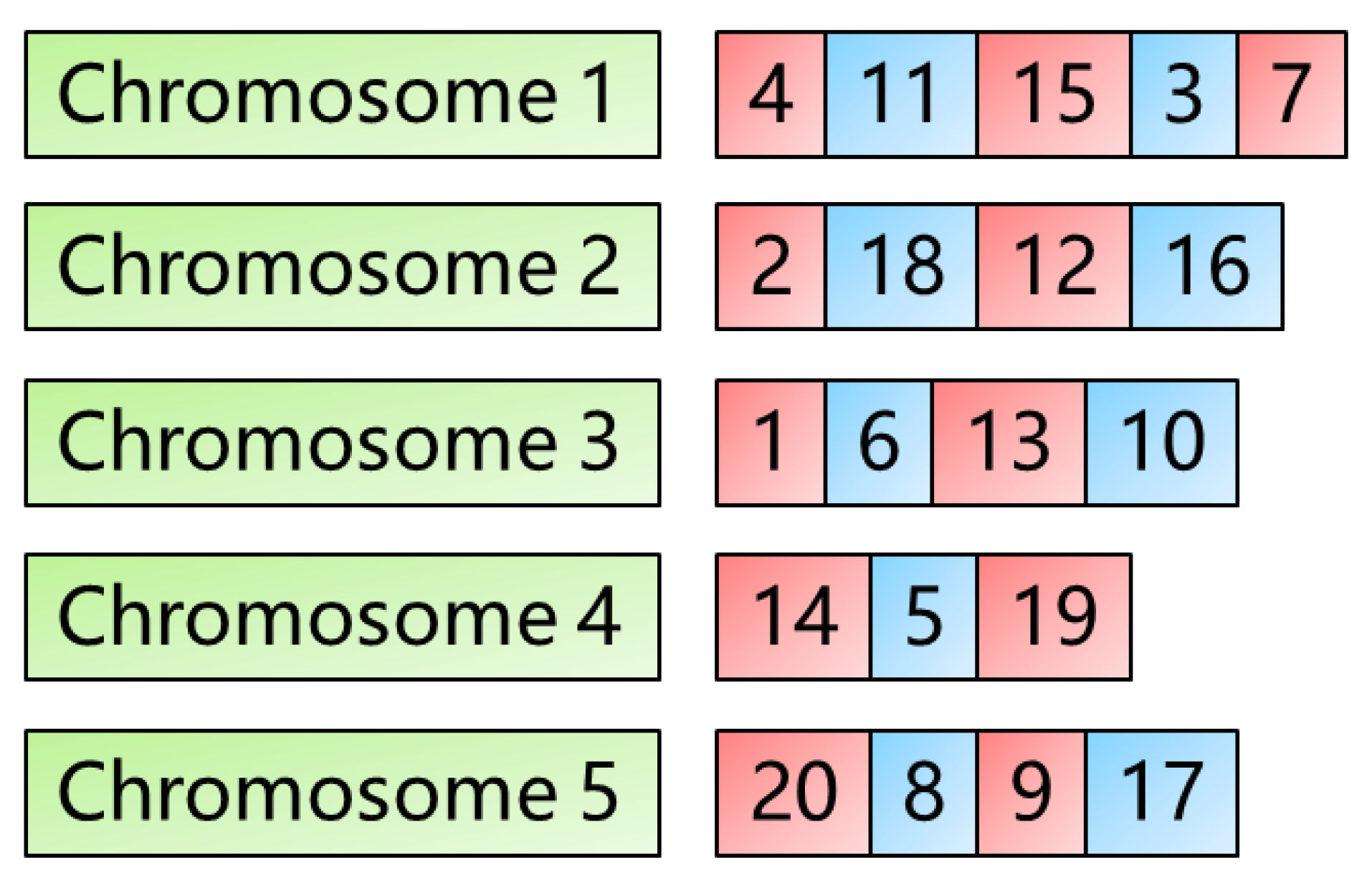
• Multi-chromosome coding-based genetic algorithms are implemented to solve large-scale multi-robot task assignment problems.

The remainder of this paper is structured as follows. Section 2 gives the problem description and the two-objective ILP model. Section 3 presents the small-scale and large-scale experiments’ results and discussions. Section 4 provides the conclusions.

2. Methods

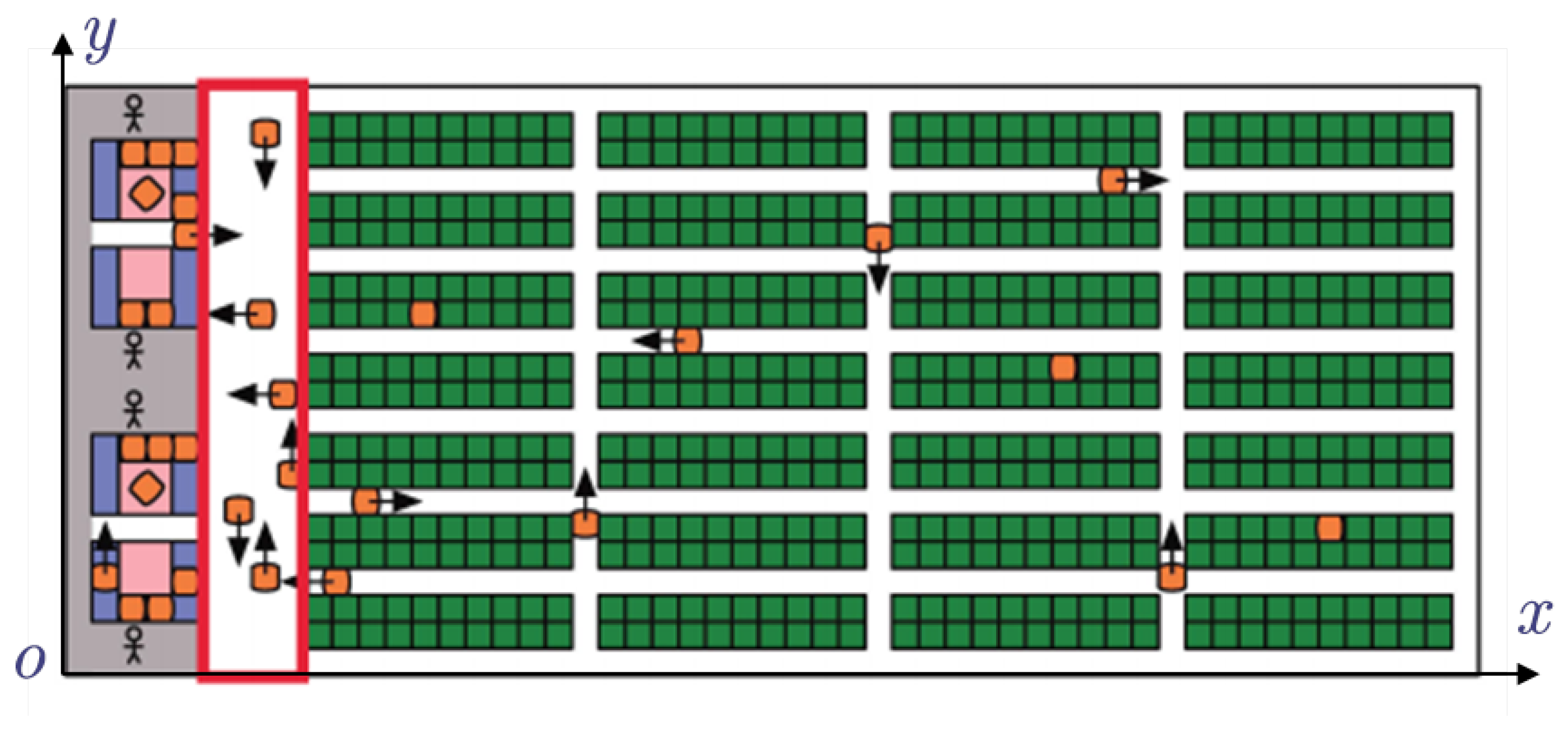
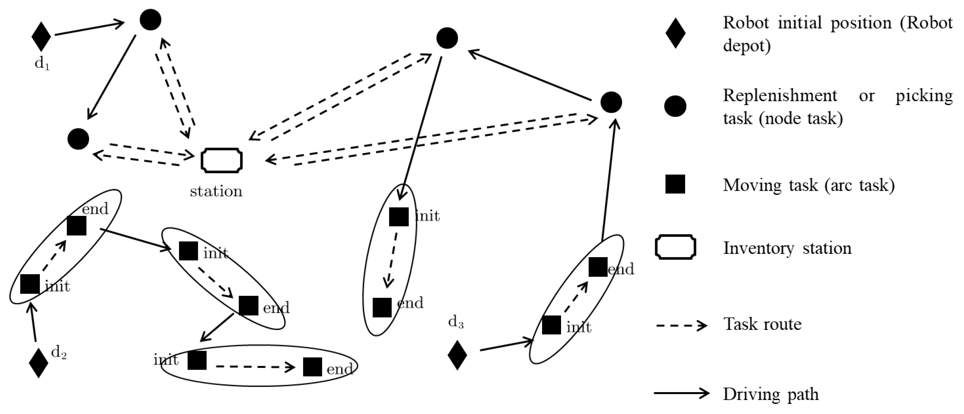
2.1. Task Definition

A warehouse task is determined by the initial position of the inventory pod, the end position of the inventory pod, and the position of the picking (replenishment) station. We use a six-dimensional coordinate to define the warehouse task as:

$$\begin{array}{c}\hfill t=(x_{init},y_{init},x_{end},y_{end},x_{station},y_{station})\end{array}$$

(1)

where $x_{init},y_{init}$ represents the initial position of the inventory pod, $x_{end},y_{end}$ represents the end position of the inventory pod, and $x_{station},y_{station}$ represents the position of the picking or replenishment station.

We define two kinds of task cost: task own cost ($TOC$) and task-associated cost ($TAC$). $TOC$ is the cost for the robot to complete a task. $TAC$ is the cost for a robot to go to another task from the current task. The distance a robot travels to complete a task can be seen as the task cost. In an intelligent warehouse, the robot can only move straight in the narrow passages between the inventory pods, so we can use the Manhattan distance to calculate the task cost. Then $TOC$ of the node task and arc task can be defined as:

$$\begin{array}{cc}\hfill TOC\left(t_{node}\right)& =2\left|x_{init}-x_{station}\right|\hfill \\ \hfill & +2\left|y_{init}-y_{station}\right|\hfill \end{array}$$

(2)

$$\begin{array}{cc}\hfill TOC\left(t_{arc}\right)& =\left|x_{init}-x_{end}\right|+\left|y_{init}-y_{end}\right|\hfill \end{array}$$

(3)

The $TAC$ from task t to task $t^{\prime }$ is the Manhattan distance between the end position of task t and the initial position of another task $t^{\prime }$. It can be defined as:

$$\begin{array}{c}\hfill TAC(t,t^{\prime })=|x_{end}-x_{init}^{\prime }|+|y_{end}-y_{init}^{\prime }|\end{array}$$

(4)

where t and $t^{\prime }$ can represent the node task and arc task.

2.2. Multi-Robot Task Assignment in an Intelligent Warehouse

Figure 4 is a diagram of task sequences for the multi-robot task assignment in an intelligent warehouse. There are 5 robots and 15 tasks, including 10 node tasks and 5 arc tasks. The task sequences of robots are $〈r_1,12,4,13,9〉$, $〈r_2,1,14〉$, $〈r_3,6,8,2〉$, $〈r_4,7,11〉$, and $〈r_5,10,5,0,3〉$. Each robot starts from a different position to complete tasks and does not return to its start position. Each task can be completed only once by one robot. Each task has a unique $TOC$. The $TAC$ between node task t and arc task $t^{\prime }$ is closely related to the task execution order, that is, $TAC\left(t,t^{\prime }\right)\ne TAC\left(t^{\prime },t\right)$. This paper contains two optimization objectives: sum-of-cost and makespan. The sum-of-cost is the sum of $TOC$ and $TAC$ for all tasks. Makespan is the maximum value of the sum of $TAC$ and $TOC$ for the tasks in each sequence. In a specific time window, when the number and type of all tasks are confirmed, the $\sum TOC$ is a constant. Therefore, the value of sum-of-cost is mainly determined by the $TAC$ of all tasks, while makespan is related to the $TOC$ and $TAC$ of the tasks in each sequence.

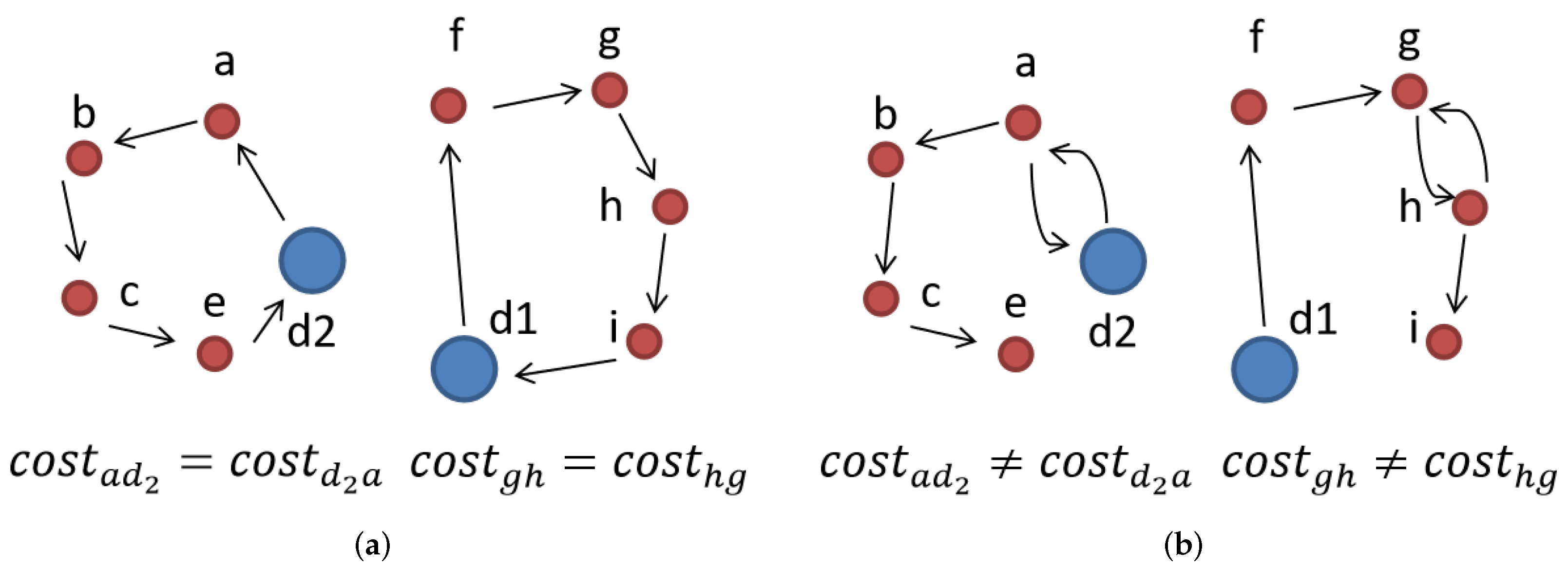
2.3. Open-Path Multi-Depot Asymmetric Traveling Salesman Problem (OP-MATSP)

We can model the multi-robot task assignment in an intelligent warehouse as an open-path multi-depot asymmetric traveling salesman problem (OP-MATSP). Each task is considered to be a city node, each robot is considered to be a traveling salesman, and the initial position of a robot is considered to be a starting depot.

OP-MATSP is another variant of TSP, consisting of m traveling salesmen, m depots, and n city nodes. Only one traveling salesman can visit each city node. The mth traveling salesman starts from the mth depot to visit respective city nodes until m traveling salesmen visit all city nodes. Each traveling salesman stays at the last city node without returning to the starting depot. OP-MATSP can be described as a directed weighted graph $G=\left(V,A\right)$ with set $V=V_n\cup V_m$ and set A. $V=\left\{1,\cdots ,n,n+1,\cdots ,n+m\right\}$ is the city node and depot set. $A=\left\{\left(i,j\right)|i,j\in V,i\ne j\right\}$ is the arc set. Subset $V_n=\left\{1,\cdots ,n\right\}$ represents n city nodes. Subset $V_m=\left\{n+1,\cdots ,n+m\right\}$ represents m depots. $C=\left(c_{ij}\right)$ is the cost matrix associated with each arc $\left(i,j\right)\in A$, and $c_{ij}\ne c_{ji}$ (asymmetric).

2.4. Formulation of the Two-Objective ILP Model

In this section, a two-objective integer linear programming (ILP) model of OP-MATSP is established. We first propose the sets, parameters, decision variables, constraints, and objective function of the two-objective integer linear programming (ILP) model for the multi-depot asymmetric traveling salesman problem (MATSP). Then, we can give the two-objective ILP model for OP-MATSP by changing the objective function.

(1)

Sets

$V_n$: the city node set.

$V_m$: the depot node set. Since each traveling salesman starts from a unique depot node, we assume that the set of traveling salesmen is equal to the depot node set $V_m$.

V: the city and depot node set.

(2)

Parameters

$c_{ij}$: the cost from node i to node j.

$q_i$: the own cost of city node i.

(3)

Decision variables

$x_{ij}^m$: if mth traveling salesman visits the node i and moves to the next node j, then $x_{ij}^m=1$; otherwise, $x_{ij}^m=0$, $i,j\in V$, $m\in V_m$.

$y_i^m$: if mth traveling salesman visits the node i, then $y_i^m=1$; otherwise, $y_i^m=0$, $i\in V$, $m\in V_m$.

(4)

Constraints

(a)

The mth traveling salesman can only visit the city node from the mth depot node, but not other depot nodes. To guarantee the above assumptions, we set the following constraints:

$$x_{ij}^m=x_{ji}^m=0,\forall i,j\in V_m,i\ne j,\forall m\in V_m$$

(5)

(b)

To prevent the traveling salesman from repeatedly visiting the same city node or depot node, the following constraint is established:

$$x_{ii}^m=0,\forall i\in V,\forall m\in V_m$$

(6)

(c)

The relationship between decision variables $x_{ij}^m$ and $y_i^m$ can be expressed as:

$$\sum _{j\in V}{x}_{ji}^m=y_i^m,\forall i\in V_n,\forall m\in V_m$$

(7)

$$\sum _{j\in V}{x}_{ij}^m=y_i^m,\forall i\in V_n,\forall m\in V_m$$

(8)

(d)

The number of node sequences is the same as the number of traveling salesmen. To ensure each traveling salesman visits only one node sequence, we add the following constraints:

$$\sum _{j\in V_n}{x}_{ij}^m=1,\forall i,m\in V_m$$

(9)

$$\sum _{j\in V_n}{x}_{ji}^m=1,\forall i,m\in V_m$$

(10)

(e)

The city node can only be visited by one traveling salesman. To prevent one city node from being repeatedly visited by different traveling salesmen, the following constraints are established:

$$\sum _{j\in V}\sum _{m\in V_m}{x}_{ij}^m=1,\forall i\in V_n,i\ne j$$

(11)

$$\sum _{i\in V}\sum _{m\in V_m}{x}_{ij}^m=1,\forall j\in V_n,i\ne j$$

(12)

(f)

To prevent the traveling salesman from visiting the previous node after visiting the current node, we establish the following constraints:

$$\sum _{m\in V_m}{x}_{ij}^m+\sum _{m\in V_m}{x}_{ji}^m<2,\forall i,j\in V,i\ne j$$

(13)

(g)

To ensure the continuity of node sequence and avoid the fracture of node sequence, the following flow balance constraint is established:

$$\sum _{j\in V}{x}_{ij}^m=\sum _{j\in V}{x}_{ji}^m,\forall i\in V,\forall m\in V_m$$

(14)

(h)

We need to ensure that every node is visited and each traveling salesman’s route forms a Hamiltonian cycle. To prevent sub-tours in the traveling salesman’s routing, we have to add sub-tour elimination constraints (SECs). The SECs for the MATSP in this paper are Danzig–Fulkerson–Johnson (DFJ) [24]:

$$\sum _{i,j\in \mathcal{S}}{x}_{ij}\le \left|\mathcal{S}\right|-1,2<\left|\mathcal{S}\right|\le \left|V\right|-1,\forall \mathcal{S}\subset V$$

(15)

where $\left|\mathcal{S}\right|$ represents the cardinality of subset $\mathcal{S}$, and $\left|V\right|$ represents the cardinality of set V. In each subset $\mathcal{S}$, sub-tours are prevented.

(i)

To ensure that each traveling salesman starts from the depot node and visits at least one city node, we add the following constraints:

$$\sum _{i\in V_m}\sum _{j\in V_n}{x}_{ij}^m=1,\forall m\in V_m$$

(16)

(5)

Objective optimization functions

We will first propose two objective optimization functions based on MATSP. Sum-of-cost consists of two parts: the sum of the costs of all city nodes ${\sum }_{i\in V_n}{q}_i$ and the sum of the costs between nodes in the node sequence ${\sum }_{i\in V}{\sum }_{j\in V}{\sum }_{m\in V_m}{c}_{ij}{x}_{ij}^m$. Because ${\sum }_{i\in V_n}{q}_i$ is a constant, the expression of sum-of-cost (SOC) can be simplified as:

$$min{f}_1=\sum _{i\in V}\sum _{j\in V}\sum _{m\in V_m}{c}_{ij}{x}_{ij}^m$$

(17)

Makespan is the maximum value of the total cost of each node sequence. Makespan also includes two parts: the sum of the costs of all city nodes in the sequence ${\sum }_{i\in V}{\sum }_{j\in V}{c}_{ij}{x}_{ij}^m$ and the sum of the costs between nodes in the node sequence $su{m}_{i\in V_n}{q}_i{y}_i^m$. We define the makespan as:

$$min{f}_2=\underset{m\in V_m}{max}\left\{\sum _{i\in V}\sum _{j\in V}{c}_{ij}{x}_{ij}^m+\sum _{i\in V_n}{q}_i{y}_i^m\right\}$$

(18)

Finally, we obtain the objective optimization function of OP-MATSP by changing the two objective functions of MATSP. The difference between OP-MATSP and MATSP is whether all traveling salesmen return to the depot after visiting all city nodes. Therefore, we can get two objective optimization functions of OP-MATSP by subtracting the cost of the traveling salesman returning the depot from the last city node in Equations (17) and (18).

The sum-of-cost of OP-MATSP can be expressed as:

$$min{f}_1=\sum _{i\in V}\sum _{j\in V}\sum _{m\in V_m}{c}_{ij}{x}_{ij}^m-\sum _{i\in V_n}\sum _{j\in V_m}\sum _{m\in V_m}{c}_{ij}{x}_{ij}^m$$

(19)

where ${\sum }_{i\in V_n}{\sum }_{j\in V_m}{\sum }_{m\in V_m}{c}_{ij}{x}_{ij}^m$ represents the cost from the last city node to the depot of all traveling salesmen.

The makespan of OP-MATSP can be expressed as:

$$min{f}_2=\underset{m\in V_m}{max}\left\{\sum _{i\in V}\sum _{j\in V}{c}_{ij}{x}_{ij}^m-\right.\left.\sum _{i\in V_n}\sum _{j\in V_m}{c}_{ij}{x}_{ij}^m+\sum _{i\in V_n}{q}_i{y}_i^m\right\}$$

where ${\sum }_{i\in V_n}{\sum }_{j\in V_m}{c}_{ij}{x}_{ij}^m$ represents the cost of the mth traveling salesman routing from the last city node to the depot.

(6)

The two-objective ILP model

In conclusion, a two-objective ILP model of OP-MATSP is established, through which we can solve the multi-robot task assignment in an intelligent warehouse. The entire two-objective ILP model is:

$$\begin{array}{ccc}\hfill min& f_1=\sum _{i\in V}\sum _{j\in V}\sum _{m\in V_m}{c}_{ij}{x}_{ij}^m-\sum _{i\in V_n}\sum _{j\in V_m}\sum _{m\in V_m}{c}_{ij}{x}_{ij}^m\hfill & \hfill \end{array}$$

(20)

$$\begin{array}{ccc}\hfill min& f_2=\underset{m\in V_m}{max}\left\{\sum _{i\in V}\sum _{j\in V}{c}_{ij}{x}_{ij}^{mk}-\sum _{i\in V_n}\sum _{j\in V_m}{c}_{ij}{x}_{ij}^m+\sum _{i\in V_n}{q}_i{y}_i^m\right\}\hfill & \hfill \end{array}$$

(21)

$$\begin{array}{ccc}\hfill s.t.& \sum _{j\in V_n}{x}_{ij}^m=1,\forall i,m\in V_m\hfill & \hfill \end{array}$$

(22)

$$\begin{array}{ccc}& \sum _{j\in V_n}{x}_{ji}^m=1,\forall i,m\in V_m\hfill & \hfill \end{array}$$

(23)

$$\begin{array}{ccc}& \sum _{j\in V}\sum _{m\in V_m}{x}_{ij}^m=1,\forall i\in V_n,i\ne j\hfill & \hfill \end{array}$$

(24)

$$\begin{array}{ccc}& \sum _{i\in V}\sum _{m\in V_m}{x}_{ij}^{mk}=1,\forall j\in V_n,i\ne j\hfill & \hfill \end{array}$$

(25)

$$\begin{array}{ccc}& x_{ij}^m=x_{ji}^m=0,\forall i,j,m\in V_m,i\ne j\hfill & \hfill \end{array}$$

(26)

$$\begin{array}{ccc}& x_{ii}^m=0,\forall i\in V,\forall m\in V_m\hfill & \hfill \end{array}$$

(27)

$$\begin{array}{ccc}& \sum _{m\in V_m}{x}_{ij}^m+\sum _{m\in V_m}{x}_{ji}^m\le 2,\forall i,j\in V,i\ne j\hfill & \hfill \end{array}$$

(28)

$$\begin{array}{ccc}& \sum _{j\in V}{x}_{ij}^m=\sum _{j\in V}{x}_{ji}^m,\forall i\in V,\forall m\in V_m\hfill & \hfill \end{array}$$

(29)

$$\begin{array}{ccc}& \sum _{i,j\in S}{x}_{ij}\le \left|S\right|-1,2<\left|S\right|\le \left|V\right|-1,\forall S\subset V\hfill & \hfill \end{array}$$

(30)

$$\begin{array}{ccc}& \sum _{i\in V_m}\sum _{j\in V_n}{x}_{ij}^m=1,\forall m\in V_m\hfill & \hfill \end{array}$$

(31)

$$\begin{array}{ccc}& \sum _{j\in V}{x}_{ji}^m=y_i^m,\forall i\in V_n,\forall m\in V_m\hfill & \hfill \end{array}$$

(32)

$$\begin{array}{ccc}& \sum _{j\in V}{x}_{ij}^m=y_i^m,\forall i\in V_n,\forall m\in V_m\hfill & \hfill \end{array}$$

(33)

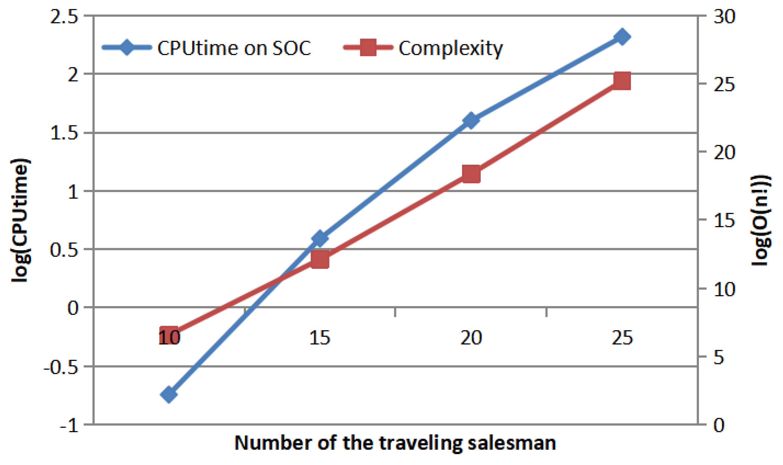
2.5. Analysis of Computational Time Complexity

Before computing the above ILP model numerically, we first perform a theoretical analysis of the OP-MATSP’s computational time complexity bound. We use the example of OP-MATSP in Figure 3b to analyze the computational time complexity bound. There are two depots, two traveling salesmen, and eight city nodes. Each depot has a traveling salesman to visit the city node. As shown in Figure 5, the traveling salesman of depot $d_1$ chooses the first city node to visit from the eight city nodes, then the traveling salesman of depot $d_2$ chooses another city node to visit from the remaining seven city nodes, until the two traveling salesmen have visited all city nodes. We can see that the bound of the computational time complexity in this example is $O(8!)$. We can then can infer that the bound of the computational time complexity of an OP-MATSP with m traveling salesmen and n city nodes is $O(n!)$.

From the computational time complexity of OP-MATSP, we can see that the computational cost of our proposed integer linear programming model is acceptable for small-scale multi-robot task assignment problems but unacceptable for large-scale problems.

3. Results and Discussion

We use Python3 for coding. The computer’s configuration is as follows: Intel Core i7 3.0 GHz processor, 32 GB RAM, and Windows 10 operating system.

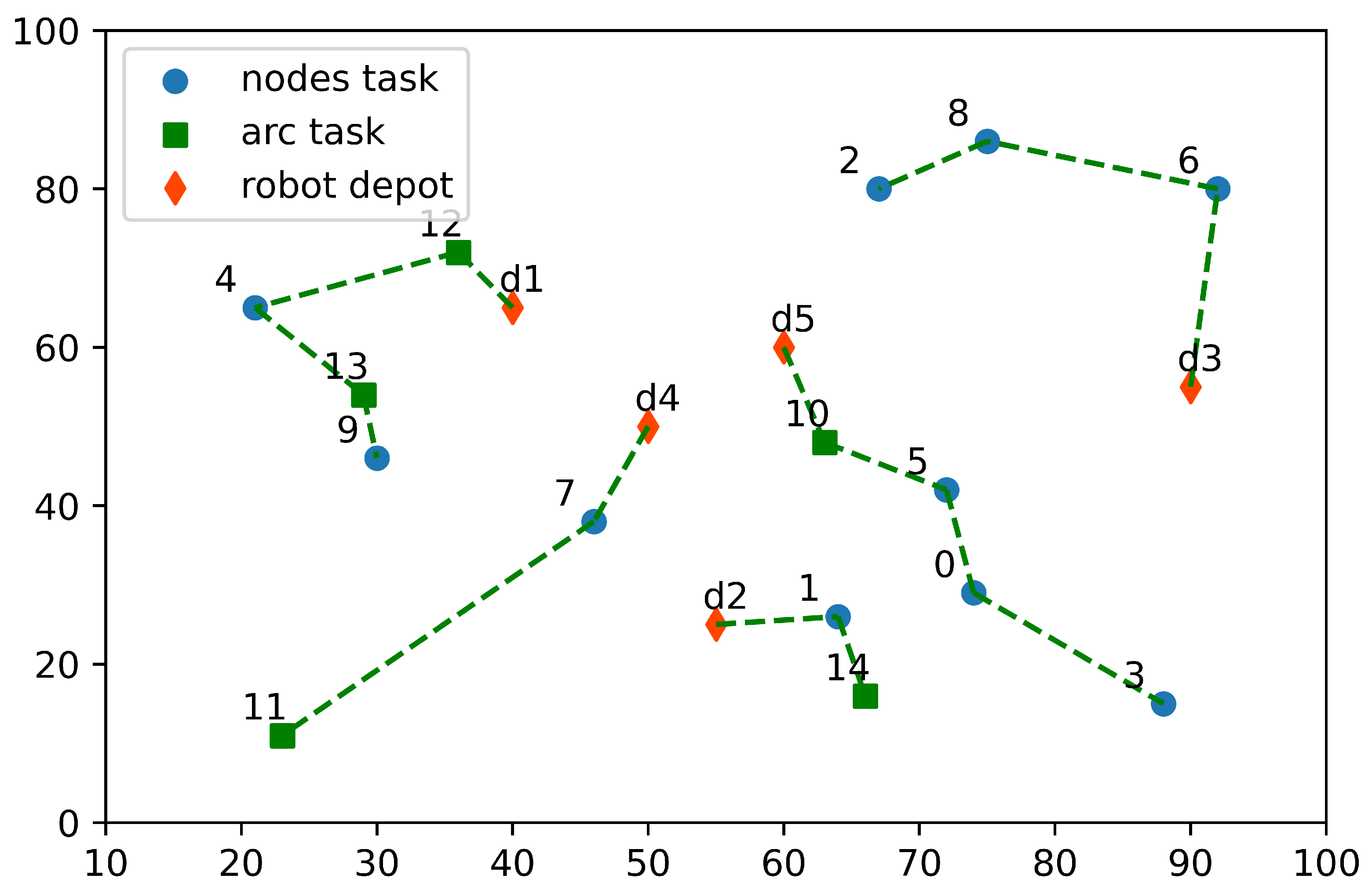
3.1. Setting and Instance Generation

The coordinates of the tasks and depots in the small-scale problems are randomly generated within the scope of 25 × 16 (m × m), while the coordinates in the large-scale problems are randomly generated within the scope 1000 × 1000 (m × m). For the small-scale problem, there are four experiment instances. They include 3 robots with 10 tasks, 3 robots with 15 tasks, 5 robots with 20 tasks, and 5 robots with 25 tasks. One experiment instance is conducted for a large-scale problem that consists of 5 robots with 100 tasks. The sum-of-cost (SOC) obtained in the following experiments does not contain the $TOC$ of all tasks.

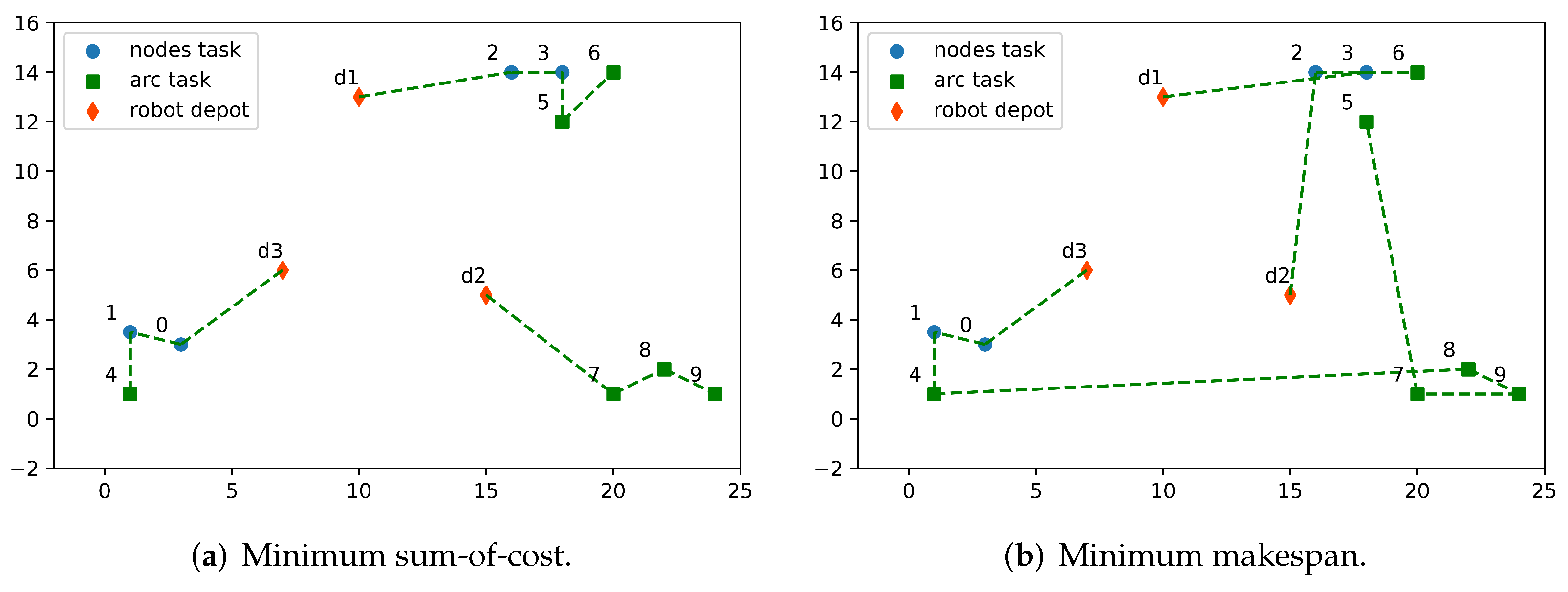
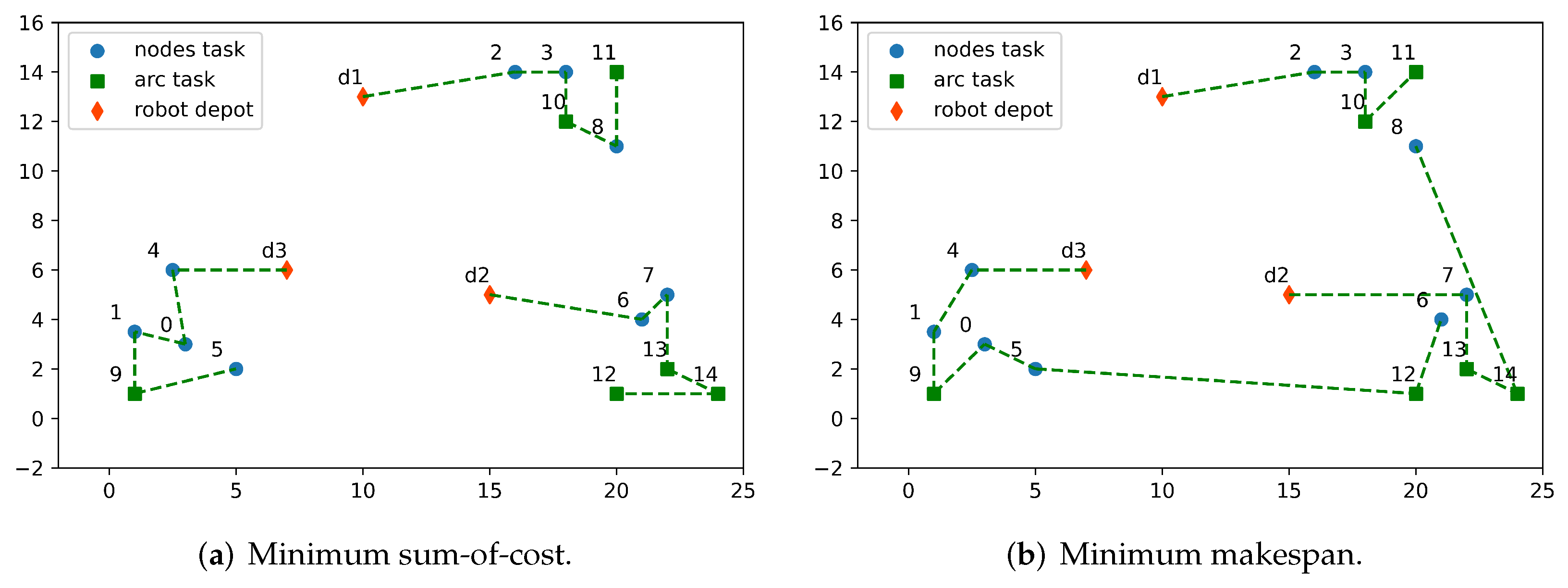
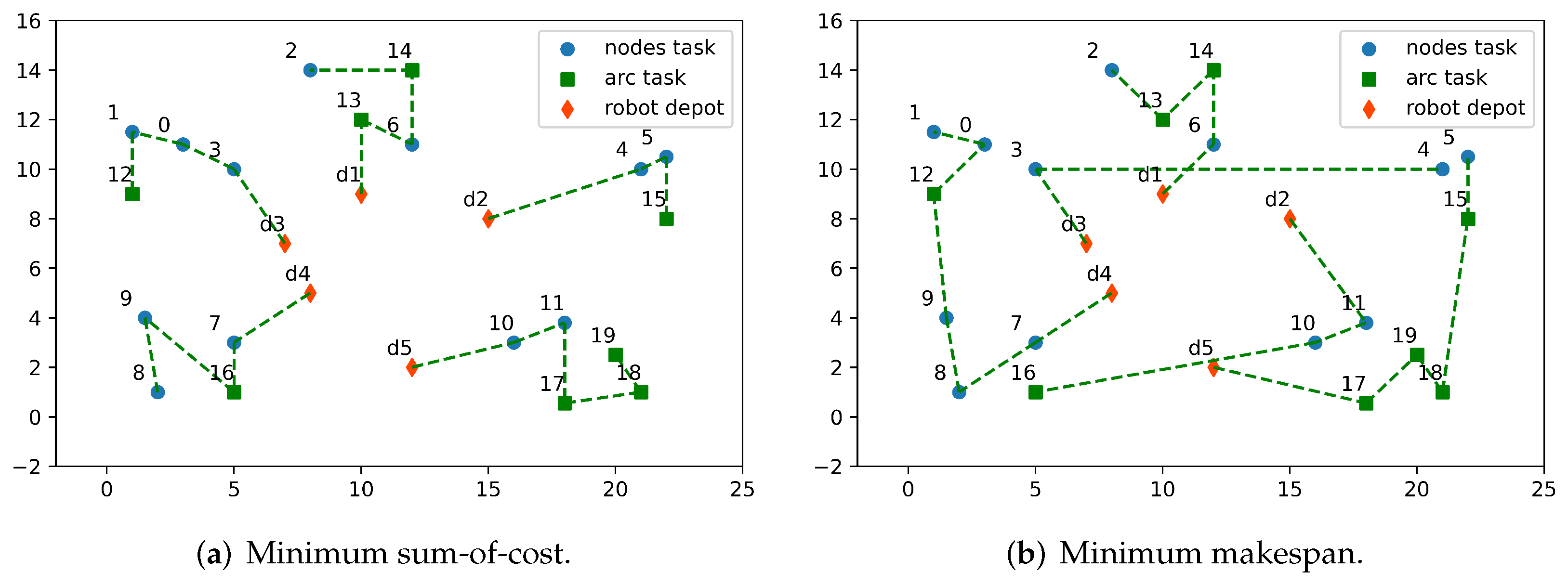
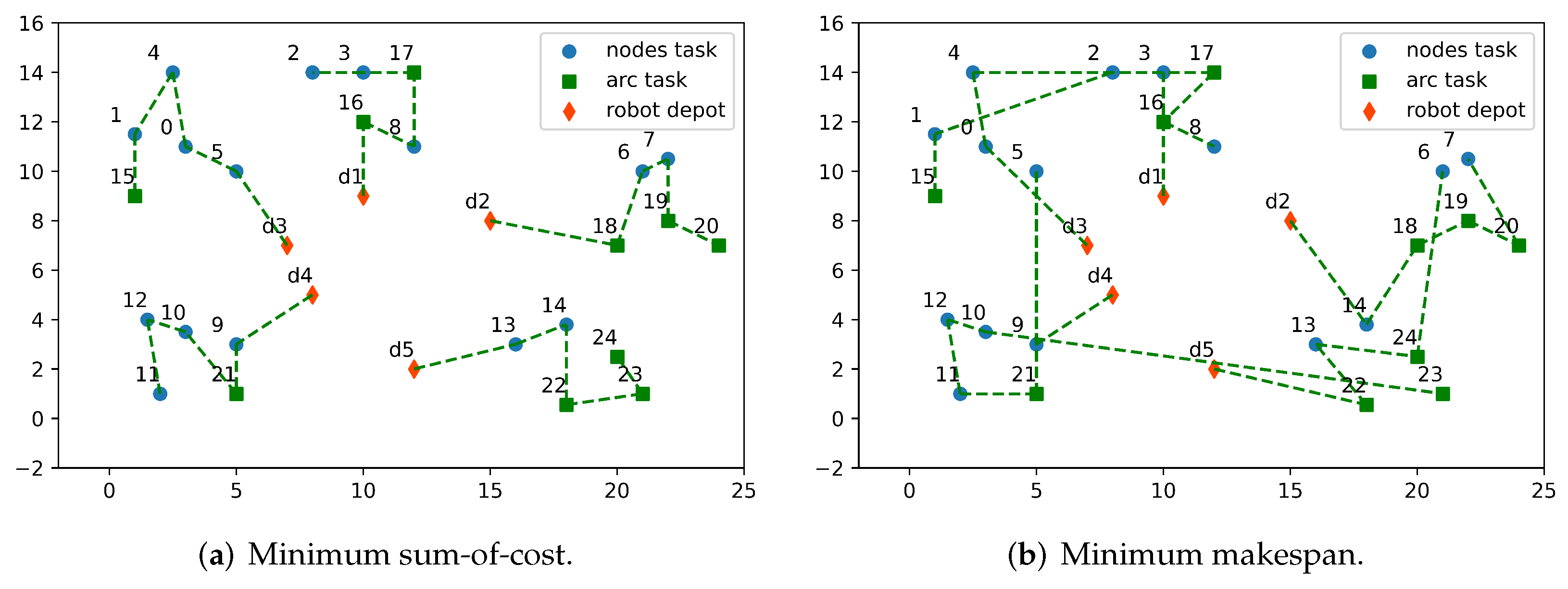
3.2. Small-Scale Problems Solved by Gurobi

This section uses the Gurobi solver to solve the small-scale multi-robot task assignment problem. First, we use the linear weighting method to give different weight coefficients $w_1$ and $w_2$ to the objective functions (19) and (20), respectively, to form the new objective function $f_3$:

$$\begin{array}{ccc}\hfill min& f_3=w_1\times f_1+w_2\times f_2\hfill & \hfill \end{array}$$

(34)

when the weight coefficient $(w_1,w_2)$ is equal to $(1,0)$ and $(0,1)$, we get the objective function with the minimum sum-of-cost (SOC) and makespan (MS). When $w_1,w_2\in \left(0,1\right)$, sum-of-cost (SOC) and makespan (MS) are both considered in the new objective function. Then, we use the Gurobi solver to solve the new ILP model. We set the weight coefficients $(w_1,w_2)$ to $(1,0)$ and $(0,1)$ in four small-scale experiments, respectively. We set the maximum CPU runtime of the Gorubi solver to 900 s.

In order to verify the theoretical analysis of the computational time complexity in Section 2.5, we perform a statistical analysis of the CPU running time of the Gurobi solver in four small-scale experiments.

Table 1. The computer’s CPU runtime and the computational time complexity.

Item	Ex-1	Ex-2	Ex-3	Ex-4
${\mathrm{CPUtime}}_{SOC}$	0.18	3.9	39.97	208.45
${\mathrm{CPUtime}}_{MS}$	1.08	362.08	900.57 1	900.4 1
$O\left(n!\right)$	10!	15!	20!	25!

¹ The CPU runtime reaches the set threshold of 900 s.

shows that as the scope of the experiment grows, the minimum SOC and minimum MS-based CPU runtimes grow longer. Furthermore, the CPU runtime based on minimum makespan (MS) is longer than that based on minimal sum-of-cost (SOC) in the same experiment. Figure 6 compares the CPU runtime based on the minimum SOC and the computational time complexity of the same experiment. The left and right vertical axes are the logarithmic values of CPU runtime and computational time complexity based on the minimum SOC, respectively. We can see that the growth trend of the above two curves is consistent with the increase of the problem size, which further verifies that our theoretical analysis of the computational time complexity is correct.

Figure 7, Figure 8, Figure 9 and Figure 10 represent the task sequence of each robot in the small-scale experiment instances, respectively. Because the solution result based on the minimum sum-of-cost (SOC) is only related to the $TAC$ between tasks and has nothing to do with the $TOC$ of the task itself, the task nodes appear to cluster in Figure 7a, Figure 8a, Figure 9a and Figure 10a. The solution results obtained based on the minimum makespan (MS) are not only related to $TAC$ but also $TOC$, so the task sequences are chaotic without the evident cluster phenomenon in Figure 7b, Figure 8b, Figure 9b and Figure 10b.

To explore the practical significance of the task assignment method in this paper, we compare it with single-task assignment (STA). Most of the existing intelligent warehouses adopt single-task assignment (STA). The approach based on the nearest distance between the start point of the task and the idle robot is more widely adopted. We now simulate it using the following method. First, we assign a task to the robot that is closest to the task starting position. Then, when a robot completes the task, we give the next task to the robot based on the nearest distance. When all tasks within the time window are given to all robots, we end the simulation process.

Based on the above four small-scale experiments, we compare the task assignment method based on the integer programming (ILP) model with the single-task assignment based on the nearest distance. In the nearest-distance-based single-task assignment, after the robot completes the task, it selects the nest task with the nearest distance to itself each time. Essentially, the single-task assignment gets a local optimal solution. In each task time window, the integer-linear-programming-based multi-task assignment (MTA) determines the execution order of tasks according to the relationship between tasks, which will obtain an optimal solution. We use Gap to represent the difference of sum-of-cost (SOC) or makespan (MS) obtained by single-task assignment (STA) based on the nearest distance and the ILP model. The expression of the Gap for sum-of-cost (SOC) and makespan (MS) is:

$$\begin{array}{c}\hfill Ga{p}_{SOC}=\left(SO{C}_{\mathrm{STA}}-SO{C}_{\mathrm{ILP}}\right)/SO{C}_{\mathrm{STA}}\end{array}$$

(35)

$$\begin{array}{c}\hfill Ga{p}_{MS}=\left(M{S}_{\mathrm{STA}}-M{S}_{\mathrm{ILP}}\right)/M{S}_{\mathrm{STA}}\end{array}$$

(36)

The results are shown in

Table 2. Comparison of single-task assignment (STA) and ILP-model-based task assignment for small-scale experiments.

Index	Item	Ex-1	Ex-2	Ex-3	Ex-4
SOC	STA	345	598.5	773	889.05
	ILP model	192	399	517.1	622.1
	$Ga{p}_{SOC}$	44.3%	33.3%	33.1%	30%
MS	STA	135	229	227	277.6
	ILP model	77	143	113	139
	$Ga{p}_{MS}$	43%	37.6%	50.2%	49.9%

. The minimum sum-of-cost (SOC) and makespan (MS) obtained by the ILP model is reduced by at least 30% and 37.6%, respectively, compared to the nearest-distance-based single-task assignment (STA), and even by 44.3% and 50.2% in some cases. The results show that the integer linear programming (ILP)-based multi-task assignment (MTA) has great advantages over the single-task assignment method based on the nearest distance for small-scale problems.

To further explore the task assignment of each robot in the four small-scale experiments, the cost of each robot’s task sequence is represented by a histogram under the patterns of $\left(w_1,w_2\right)=\left(1,0\right)$, $\left(w_1,w_2\right)=\left(0,1\right)$, and single-task assignment (STA). As shown in Figure 11, when $\left(w_1,w_2\right)=\left(0,1\right)$, the total cost of each robot’s task sequence is relatively balanced and the value of makespan (MS) is the smallest. When $\left(w_1,w_2\right)=\left(1,0\right)$, the sum-of-cost (SOC) is the smallest. For the single-task assignment (STA) based on the nearest distance, the values of sum-of-cost (SOC) and makespan (MS) are larger than the other two task assignment patterns.

From the above analysis, we know that the two-objective integer linear programming (ILP)-based multi-robot task assignment in this paper has practical significance and can significantly improve the operating efficiency and reduce the operating cost of an intelligent warehouse.

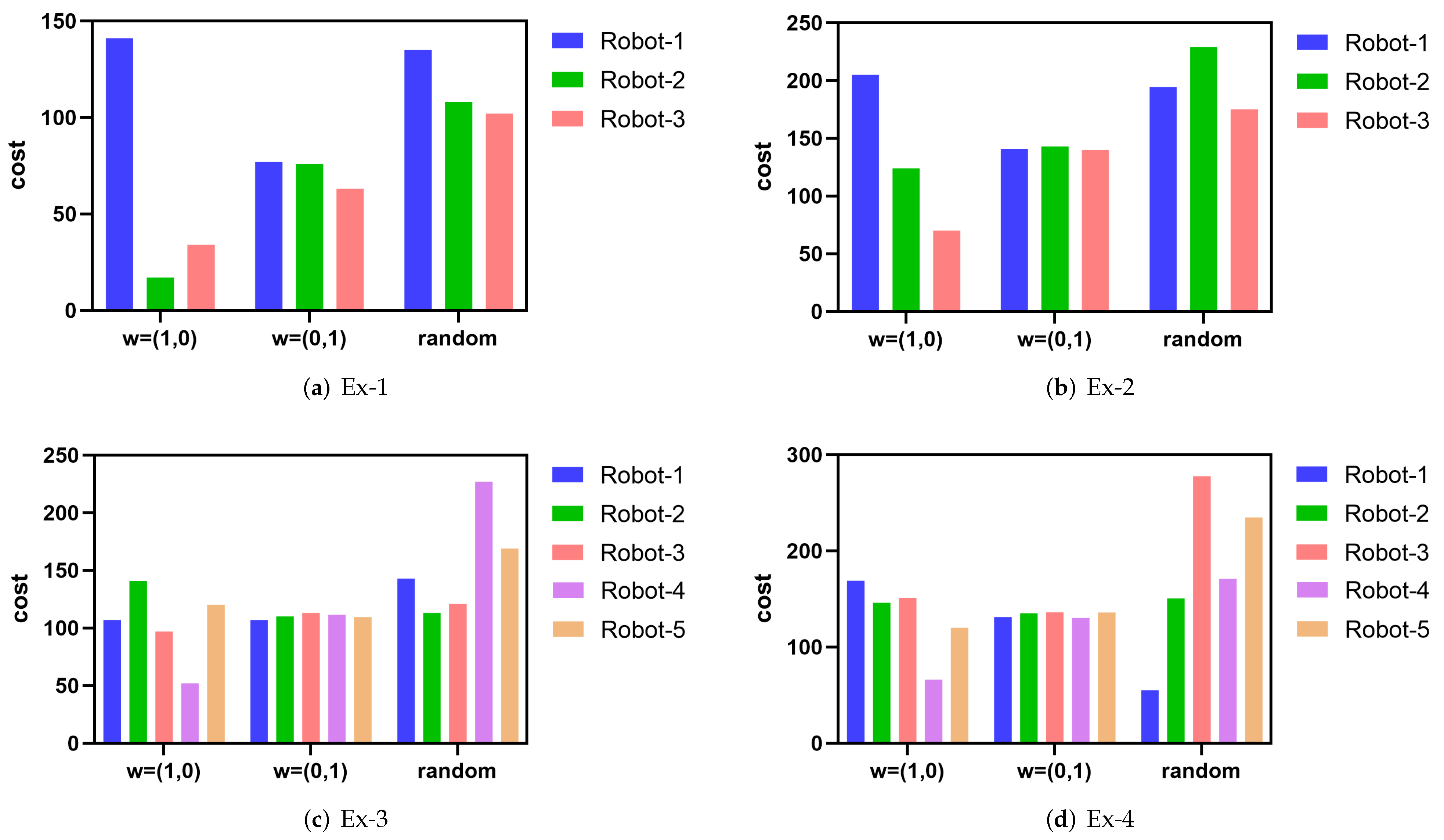
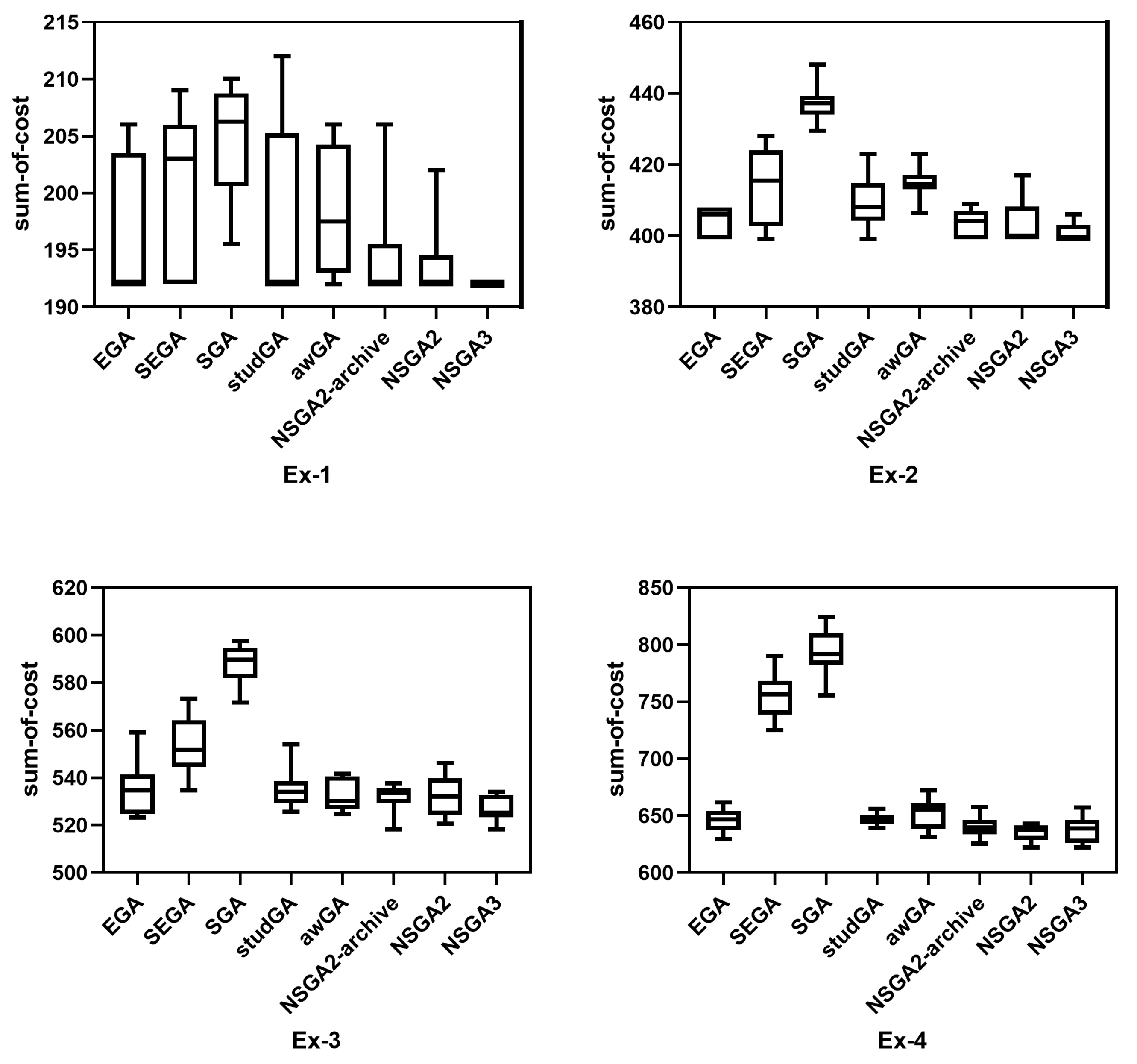
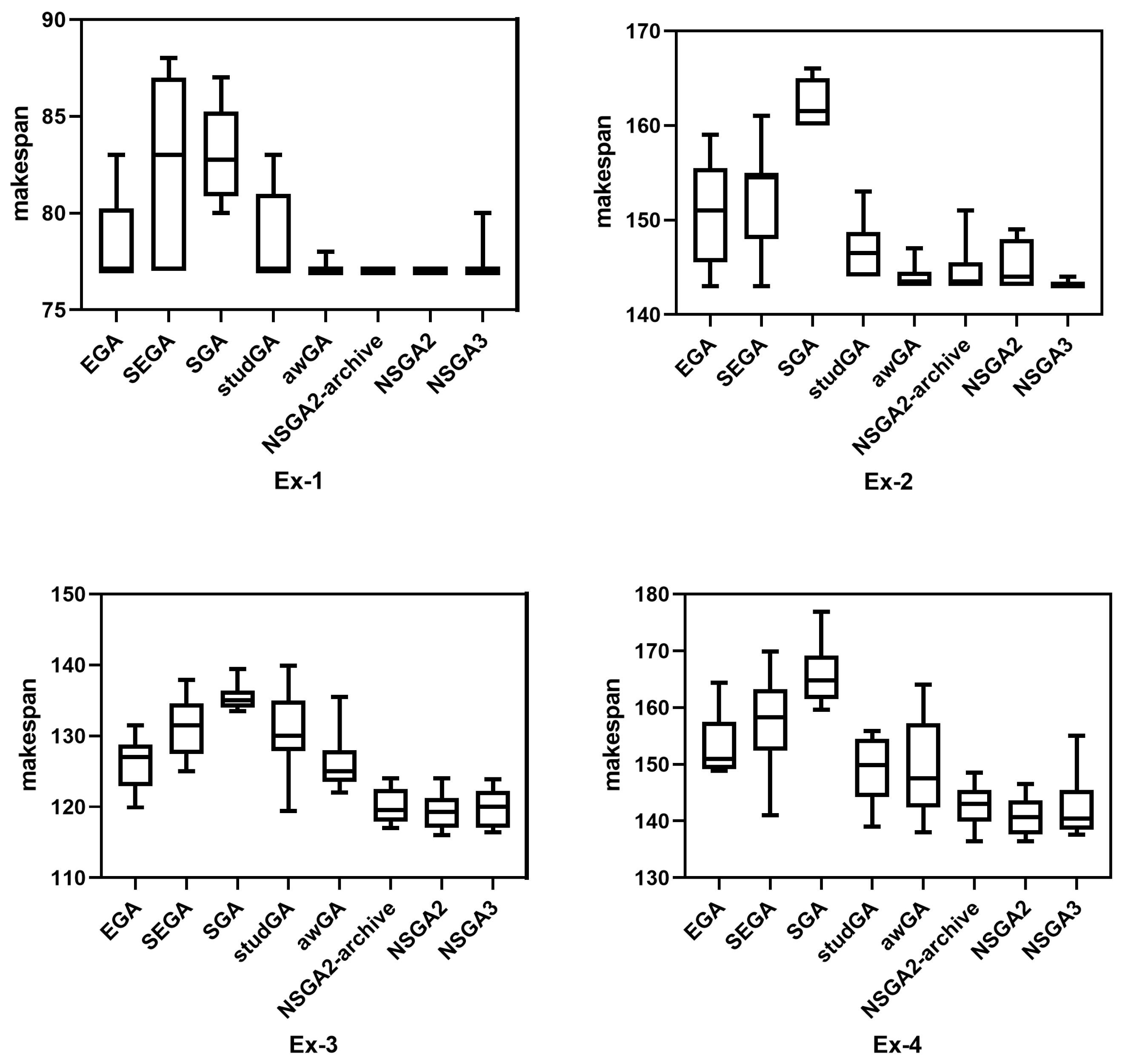
3.3. Large-Scale Problems Solved by the Multi-Chromosome Coding-Based Genetic Algorithm

For large-scale problems, multi-chromosome coding-based genetic algorithms are implemented. This kind of genetic algorithm not only has a smaller search space [30] but also facilitates the integer coding for the multi-robot task assignment.

The multi-chromosome coding-based genetic algorithm also includes chromosome coding, population initialization, selection, crossover, mutation, and other processes. First, the integer coding process of the multi-chromosome genetic algorithm is described. The number of chromosomes of each individual in the population is equal to the number of robots. For a multi-robot task assignment problem containing n tasks and m robots, the task set is $V_n$, and the robot set is $V_m$. Each task represents a gene. Each individual in the population contains m chromosomes. The sequence of genes represents the order of tasks. After many generations of evolution, we pick out the best individuals from the population and assign them to robots. Then, 5 robots and 20 tasks are used to illustrate the multi-chromosome integer coding process, as shown in Figure 12. The specific generation process of a random initial population of size S is as follows: First, the order of the original task sequence needs to be disrupted, and then a robot is randomly chosen and assigned the first task of the new task sequence. It then randomly chooses a robot from all the robots and gives the second task to that robot. When all tasks are assigned, the individual of the population will be retained if every robot has at least one task. Otherwise, it will be discarded and re-assigned. The process is repeated until the population size reaches S. The objective function (34) is used to evaluate the population’s individual. When weight coefficient $(w_1,w_2)$ is equal to $(1,0)$ and $(0,1)$, respectively, we get the best individual of the population with the minimum sum-of-cost (SOC) and makespan (MS).

We use the multi-chromosome coding-based genetic algorithm in the GEATPY library to solve the large-scale multi-robot task assignment problem. GEATPY is a high-performance genetic algorithm library, which can be found on https://github.com/geatpy-dev/geatpy (accessed on 1 January 2022). We first test the eight kinds of multi-chromosome coding-based genetic algorithms on the small-scale experiment instances. Eight kinds of multi-chromosome coding-based genetic algorithms are shown in

Table 3. Multi-chromosome coding-based genetic algorithm templets of GEATPY.

Type	Templet	Selection	Crossover	Mutation
Single-obj	soea_psy_EGA_templet 1	Tournament	partial matching ($P_c=0.7$)	Invertion ($P_m=0.5$)
	soea_psy_SEGA_templet 2	Tournament	partial matching ($P_c=0.7$)	Invertion ($P_m=0.5$)
	soea_psy_SGA_templet 3	Roulette Wheel	partial matching ($P_c=0.7$)	Invertion ($P_m=0.5$)
	soea_psy_studGA_templet [31]	Tournament	partial matching ($P_c=0.7$)	Invertion ($P_m=0.5$)
Multi-obj	moea_psy_awGA_templet 4	Tournament	partial matching ($P_c=1$)	Invertion ($P_m=1$)
	moea_psy_NSGA2_templet [32]	Tournament	partial matching ($P_c=1$)	Invertion ($P_m=1$)
	moea_psy_NSGA2_archive_templet 5	Tournament	partial matching ($P_c=1$)	Invertion ($P_m=1$)
	moea_psy_NSGA3_templet [33]	unconstrained random	partial matching ($P_c=1$)	Invertion ($P_m=1$)

¹ This is the elitist reservation GA algorithm. ² This is the strengthen elitist reservation GA algorithm. ³ This is the simple GA algorithm. ⁴ This is the multi-objective awGA algorithm. ⁵ This is the NSGA-II algorithm with global archive.

, including four types of single-objective and four types of multi-objective. Selection strategies of genetic algorithms include tournament, roulette wheel, and unconstrained random. We choose the partial matching crossover and reverse mutation operators that come with the GEATPY library for both crossover and mutation operators. We choose partial matching crossover and reverse mutation operators for both crossover and mutation operators. Regarding the crossover probability and mutation probability, we choose $P_c=0.7$ and $P_m=0.5$ in the single-objective genetic algorithm, respectively, and $P_c=1$ and $P_m=1$ in the multi-objective genetic algorithm. The iteration number of the genetic algorithm is 5000, and the population size is 100.

Then, we compare this with the results of the ILP model using the Gurobi solver, respectively. The experiment instances with different weight coefficients and different genetic algorithms are repeated 10 times, respectively. In each small-scale experiment, we statistically obtain the best and average values of sum-of-cost (SOC) and makespan (MS) from 10 repetitions of the genetic algorithms. We use Gap to represent the difference of sum-of-cost (SOC) or makespan (MS) obtained by the multi-chromosome coding-based genetic algorithm (GA) and the ILP model. The expression of Gap for sum-of-cost (SOC) and makespan (MS) is:

$$\begin{array}{c}\hfill Ga{p}_{SOC}=\left(SO{C}_{\mathrm{GA}}-SO{C}_{\mathrm{ILP}}\right)/SO{C}_{\mathrm{GA}}\end{array}$$

(37)

$$\begin{array}{c}\hfill Ga{p}_{MS}=\left(M{S}_{\mathrm{GA}}-M{S}_{\mathrm{ILP}}\right)/M{S}_{\mathrm{GA}}\end{array}$$

(38)

The comparison results of the multi-chromosome coding-based genetic algorithm and the ILP model are shown in

Table 4. Comparison results of the multi-chromosome coding-based genetic algorithms and ILP model in the small-scale experiments.

Ex	Index	soea-EGA		soea-SEGA		soea-SGA		soea-studGA		moea-awGA		moea-NSGA2-archive		moea-NSGA2		moea-NSGA3
		Best	Aveg	Best	Aveg	Best	Aveg	Best	Aveg	Best	Aveg	Best	Aveg	Best	Aveg	Best	Aveg
Ex-1	SOC	192	195.8	192	200.1	195.5	204.6	192	196.7	192	198.2	192	194.6	192	196.5	192	192
	$Ga{p}_{SOC}$	0%	1.94%	0%	4.05%	1.79%	6.16%	0%	2.39%	0%	3.13%	0%	1.34%	0%	1.03%	0%	0%
	MS	77	78.6	77	82.1	80	83	77	78.7	77	77.1	77	77	77	77	77	77.3
	$Ga{p}_{MS}$	0%	2.04%	0%	6.21%	3.75%	7.23%	0%	2.16%	0%	0.13%	0%	0%	0%	0%	0%	0.39%
Ex-2	SOC	399	403.9	399	414.1	429.5	437.4	399	409.1	406.5	414.7	399	403.65	399	403.7	399	400.7
	$Ga{p}_{SOC}$	0%	1.21%	0%	3.65%	7.1%	8.78%	0%	2.47%	1.85%	3.79%	0%	1.15%	0%	1.16%	0%	0.42%
	MS	143	150.6	143	152.2	160	162.3	144	146.9	143	144	143	144.6	143	145.09	143	143.2
	$Ga{p}_{MS}$	0%	5.05%	0%	6.04%	10.63%	11.89%	0.69%	2.65%	0%	0.69%	0%	1.11%	0%	1.58%	0%	0.14%
Ex-3	SOC	523.25	535.12	534.6	552.99	571.6	588.21	525.5	534.92	524.6	531.98	518.1	532.15	520.6	531.93	518.1	526.97
	$Ga{p}_{SOC}$	1.18%	3.37%	3.27%	6.49%	9.53%	12.09%	1.6%	3.33%	1.43%	2.8%	0.19%	2.83%	0.67%	2.79%	0.19%	1.87%
	MS	119.9	126.17	125	131.33	133.5	135.53	119.4	130.93	122	126.25	117	120.05	116	119.36	116.4	120
	$Ga{p}_{MS}$	5.75%	10.44%	9.6%	13.96%	15.36%	16.62%	5.36%	13.69%	7.38%	10.5%	3.42%	5.87%	2.59%	5.33%	2.92%	5.38%
Ex-4	SOC	629	645.53	725	755.09	755.6	793.1	639.1	647.16	631.1	652.01	625.5	640.31	622.1	635.6	622.1	637.89
	$Ga{p}_{SOC}$	1.1%	3.63%	14.19%	17.61%	17.67%	21.56%	2.66%	3.87%	1.43%	4.59%	0.54%	2.84%	0%	2.12%	0%	2.48%
	MS	148.9	153.5	141	157.29	159.6	165.84	139	149.13	138	149.8	136.4	142.63	136.4	140.73	137.6	142.44
	$Ga{p}_{MS}$	6.65%	9.45%	1.42%	11.63%	12.91%	16.18%	0%	6.79%	−0.72%	7.21%	−1.91%	2.55%	−1.91%	1.23%	−1.02%	2.42%

. In the same experiment, the Pareto frontier extreme values obtained from the multi-objective genetic algorithm are equal to or close to the results obtained by the Gurobi solver. The best value of makespan obtained by awGA, NSGA2, NSGA2-archive, and NSGA3 in experiment 4 is smaller than the result obtained by the Gurobi solver. This indicates that when the problem scale reaches 5 robots and 25 tasks, the best value obtained by some genetic algorithms is better than that of the Gurobi solver.

To make it easier to compare the performance of each genetic algorithm in the four small-scale experiments, we use box-whisker plots to display the results. Based on Table 4, the box-whisker plots on the minimum sum-of-cost (SOC) and makespan (MS) are shown in Figure 13 and Figure 14. It can be seen that as the number of robots and tasks increases, the Gap between the maximum and minimum results obtained by the same genetic algorithm becomes larger under the same number of iterations. The stability of the solution results gradually deteriorates. Among the eight tested genetic algorithms, the algorithms of EGA and NSGA3 perform relatively better. Therefore, we next choose these two algorithms to solve the large-scale problems.

The large-scale experiment instance includes 5 robots and 100 tasks. We use the two algorithms to solve the experimental case 10 times. To further explore the influence of the number of iterations of the genetic algorithm on the solution results, we set the number of iterations to 5000 and 20,000, respectively. The other parameters are the same as those of the small-scale experiment. We use the Gap to represent the difference between sum-of-cost (SOC) or makespan (MS) when the number of iterations is 5000 and 20,000. The expression of the Gap for sum-of-cost (SOC) and makespan (MS) is:

$$\begin{array}{c}\hfill Ga{p}_{SOC}=\left(SO{C}_{5000}-SO{C}_{20,000}\right)/SO{C}_{5000}\end{array}$$

(39)

$$\begin{array}{c}\hfill Ga{p}_{MS}=\left(M{S}_{5000}-M{S}_{20,000}\right)/M{S}_{5000}\end{array}$$

(40)

As shown in

Table 5. Large-scale experiment results by genetic algorithms.

Index	Interation	EGA		NSGA3
		Best	Aveg	Best	Aveg
SOC	5000	186,274	188,044	183,507	185,334
	20,000	182,712	184,076	182,074	184,494
	$Ga{p}_{SOC}$	1.91%	2.11%	0.78%	0.45%
MS	5000	40,410	42,021	37,241	37,836.2
	20,000	39,552	40,455.3	37,272	37,795.7
	$Ga{p}_{MS}$	2.12%	3.73%	−0.08%	0.11%

, when the number of iterations is 5000 and 20,000, the Gaps between the best value and the average values of the sum-of-cost (SOC) and makespan (MS) obtained by the EGA algorithm are all less than 4%. For the NSGA3 algorithm, the Gap is less than 1%. The results show that the two genetic algorithms have achieved good sub-optimal results when the number of iterations is 5000. They can be applied to other large-scale multi-robot task assignment problems of the intelligent warehouse. When the number of robots and tasks grows, we should appropriately increase the number of iterations of the genetic algorithm to obtain better results.

4. Conclusions

This paper proposes a two-objective integer linear programming (ILP) model of open-path multi-depot asymmetric traveling salesman problem (OP-MDATSP) for the multi-robot task assignment in an intelligent warehouse. The theoretical bound on the computational time complexity of this model is $O(n!)$. Then, we transfer the two-objective linear integer programming model to a single-objective model using the linear weight method. We solve this single-objective model on a small-scale problem using the Gurobi solver, and we compare the results with the nearest distance-based single-task assignment method. The values of the minimum sum-of-cost and makespan obtained based on the ILP model are much lower than those of the the nearest-distance-based single-task assignment (STA). After testing eight kinds of different multi-chromosome coding-based genetic algorithms in four small-scale experiments, we find that two genetic algorithms, EGA and NSGA3, perform relatively better. We use them to solve the large-scale problems. The results of the large-scale experiments show that the two genetic algorithms can solve large-scale problems well. This shows that the multi-robot task assignment method proposed in this paper has great practical significance for the intelligent warehouse to reduce its operating cost. In addition, we can adjust the weight coefficients in the objective function of this paper according to the needs of the actual scene.

For the following work, we will consider the path conflicts between robots during the task assignment of the intelligent warehouse. In addition, this paper only considers task assignment in a static state, where all task points and robot positions are determined. In the future, we will consider some unexpected scenarios, such as the dynamic change of robot state and task point state, to further verify the robustness of our method. In this paper, we assume that the robot’s power is infinite and do not consider issues such as charging, which we will study in the following work.

References

1. de Koster, R. Automated and Robotic Warehouses: Developments and Research Opportunities. Logist. Transp. 2018, 38, 33–40. [Google Scholar] [CrossRef]
2. Farinelli, A.; Boscolo, N.; Zanotto, E.; Pagello, E. Advanced approaches for multi-robot coordination in logistic scenarios. Robot. Auton. Syst. 2017, 90, 34–44. [Google Scholar] [CrossRef]
3. Wurman, R.P.; D’Andrea, R.; Mountz, M. Coordinating hundreds of cooperative, autonomous vehicles in warehouses. AI Mag. 2007, 29, 1752–1759. [Google Scholar]
4. NZanywayingoma, F.; Yang, Y. Effective task scheduling and dynamic resource optimization based on heuristic algorithms in cloud computing environment. KSII Trans. Internet Inf. Syst. 2017, 11, 5780–5802. [Google Scholar]
5. Erdmann, M.; Lozano-Perez, T. On multiple moving objects. In Proceedings of the 1986 IEEE International Conference on Robotics and Automation, San Francisco, CA, USA, 7–10 April 1986; Volume 3, pp. 1419–1424. [Google Scholar] [CrossRef]
6. Wagner, G.; Choset, H.; Ayanian, N. Subdimensional Expansion and Optimal Task Reassignment. In SOCS, Proceedings of the 5th Annual Symposium on Combinatorial, Niagara Falls, ON, Canada, 19–21 July 2012; Association for the Advancement of Artificial Intelligence: Palo Alto, CA, USA, 2012. [Google Scholar]
7. Khamis, A.; Hussein, A.; Elmogy, A. Multi-robot task allocation: A review of the state-of-the-art. Coop. Robot. Sens. Netw. 2015, 2015, 31–51. [Google Scholar]
8. Liu, Y.; Ji, S.; Su, Z.; Guo, D. Multi-objective AGV scheduling in an automatic sorting system of an unmanned (intelligent) warehouse by using two adaptive genetic algorithms and a multi-adaptive genetic algorithm. PLoS ONE 2019, 14, e0226161. [Google Scholar] [CrossRef]
9. Pan, X.Y.; Wu, J.; Zhang, Q.W.; Lai, D.; Xie, H.L.; Zhang, C. A case study of AGV scheduling for production material handling. Appl. Mech. Mater. 2013, 411, 2351–2354. [Google Scholar] [CrossRef]
10. Zheng, Y.; Xiao, Y.; Seo, Y. A tabu search algorithm for simultaneous machine/AGV scheduling problem. Int. J. Prod. Res. 2014, 52, 5748–5763. [Google Scholar] [CrossRef]
11. Mousavi, M.; Yap, H.J.; Musa, S.N.; Tahriri, F.; Md Dawal, S.Z. Multi-objective AGV scheduling in an FMS using a hybrid of genetic algorithm and particle swarm optimization. PLoS ONE 2017, 12, e0169817. [Google Scholar] [CrossRef] [Green Version]
12. Su-yan, T.; Yi-fan, Z.; Li, Q.; Yong-lin, L. Survey of task allocation in multi Agent systems. Xi Tong Gong Cheng Yu Dian Zi Ji Shu [Syst. Eng. Electron.] 2010, 32, 2155–2161. [Google Scholar]
13. Axsäter, S. On the first come–first served rule in multi-echelon inventory control. Nav. Res. Logist. 2007, 54, 485–491. [Google Scholar] [CrossRef]
14. Shi, J.; Bao, Y.; Leng, F.; Yu, G. Priority-Based Balance Scheduling in Real-Time Data Warehouse. In Proceedings of the 2009 Ninth International Conference on Hybrid Intelligent Systems, Shenyang, China, 12–14 August 2009; Volume 3, pp. 301–306. [Google Scholar] [CrossRef]
15. Bolu, A.; Korçak, Ö. Adaptive task planning for multi-robot smart warehouse. IEEE Access 2021, 9, 27346–27358. [Google Scholar] [CrossRef]
16. Zhang, J.; Yang, F.; Weng, X. A building-block-based genetic algorithm for solving the robots allocation problem in a robotic mobile fulfilment system. Math. Probl. Eng. 2019, 2019, 6153848. [Google Scholar] [CrossRef] [Green Version]
17. Vivaldini, K.; Rocha, L.; Fróes, N.; Becker, M.; Moreira, A. Integrated tasks assignment and routing for the estimation of the optimal number of AGVS. Int. J. Adv. Manuf. Technol. 2015, 82, 719–736. [Google Scholar] [CrossRef]
18. Lenstra, J.K.; Kan, A.R. Some simple applications of the travelling salesman problem. J. Oper. Res. Soc. 1975, 26, 717–733. [Google Scholar] [CrossRef]
19. De Koster, R.; Le-Duc, T.; Roodbergen, K.J. Design and control of warehouse order picking: A literature review. Eur. J. Oper. Res. 2007, 182, 481–501. [Google Scholar] [CrossRef]
20. Theys, C.; Bräysy, O.; Dullaert, W.; Raa, B. Using a TSP heuristic for routing order pickers in warehouses. Eur. J. Oper. Res. 2010, 200, 755–763. [Google Scholar] [CrossRef]
21. Azadnia, H.A.; Taheri, S.; Ghadimi, P.; Saman, Z.M.M.; Wong, Y.K. Order batching in warehouses by minimizing total tardiness: A hybrid approach of weighted association rule mining and genetic algorithms. Sci. World J. 2013, 2013, 246578. [Google Scholar] [CrossRef]
22. Tsiropoulou, E.E.; Paruchuri, S.T.; Baras, J.S. Interest, energy and physical-aware coalition formation and resource allocation in smart IoT applications. In Proceedings of the 2017 51st Annual Conference on Information Sciences and Systems (CISS), Baltimore, MD, USA, 22–24 March 2017; pp. 1–6. [Google Scholar]
23. Benavent, E.; Martínez, A. Multi-depot multiple TSP: A polyhedral study and computational results. Ann. Oper. Res. 2013, 207, 7–25. [Google Scholar] [CrossRef]
24. Dantzig, G.; Fulkerson, R.; Johnson, S. Solution of a large-scale traveling-salesman problem. J. Oper. Res. Soc. Am. 1954, 2, 393–410. [Google Scholar] [CrossRef] [Green Version]
25. Odili, J.B.; Noraziah, A.; Zarina, M. A Comparative Performance Analysis of Computational Intelligence Techniques to Solve the Asymmetric Travelling Salesman Problem. Comput. Intell. Neurosci. 2021, 2021, 6625438. [Google Scholar] [CrossRef] [PubMed]
26. Bixby, B. The gurobi optimizer. Transp. Res. Part B 2007, 41, 159–178. [Google Scholar]
27. Liu, Z.; Liu, G.; Wang, H.; He, F. The linear weighting method for solving a class of non-differentiable multiobjective programming problem. In Proceedings of the 2011 International Conference on Multimedia Technology, Hangzhou, China, 26–28 July 2011; pp. 3273–3276. [Google Scholar]
28. Ronald, S.; Kirkby, S.; Eklund, P. Multi-chromosome mixed encodings for heterogeneous problems. In Proceedings of the 1997 IEEE International Conference on Evolutionary Computation (ICEC’97), Indianapolis, IN, USA, 13–16 April 1997; pp. 37–42. [Google Scholar] [CrossRef]
29. Ciesielski, V.; Scerri, P. Compound optimisation. Solving transport and routing problems with a multi-chromosome genetic algorithm. In Proceedings of the 1998 IEEE International Conference on Evolutionary Computation Proceedings. IEEE World Congress on Computational Intelligence (Cat. No. 98TH8360), Anchorage, AK, USA, 4–9 May 1998; pp. 365–370. [Google Scholar] [CrossRef]
30. Ye, D.; Liu, G.; He, B. Multi-chromosome Genetic Algorithm for Multiple Traveling Salesman Problem. J. Syst. Simul. 2019, 31, 36–42. [Google Scholar]
31. Khatib, W.; Fleming, P.J. The stud GA: A mini revolution? In Proceedings of the International Conference on Parallel Problem Solving from Nature, Amsterdam, The Netherlands, 27–30 September 1998. [Google Scholar]
32. Deb, K.; Pratap, A.; Agarwal, S.; Meyarivan, T. A fast and elitist multiobjective genetic algorithm: NSGA-II. IEEE Trans. Evol. Comput. 2002, 6, 182–197. [Google Scholar] [CrossRef] [Green Version]
33. Deb, K.; Jain, H. An Evolutionary Many-Objective Optimization Algorithm Using Reference-Point-Based Nondominated Sorting Approach, Part I: Solving Problems with Box Constraints. IEEE Trans. Evol. Comput. 2014, 18, 577–601. [Google Scholar] [CrossRef]
Figure 1. Two-dimensional schematic of Amazon’s order fulfillment center [3]. The orange squares represent the robots. The green squares represent the inventory pods. The inventory stations are shown only on the left side and are usually located around the perimeter of warehouse.
Applsci 12 04843 g001
Figure 2. The multi-robot task assignment in an intelligent warehouse.
Applsci 12 04843 g002
Figure 3. The diagram of MTSP and OP-MATSP. (a) Multi-depot traveling salesman problem (MTSP). (b) Open path multi-depot asymmetric traveling salesman problem (OP-MATSP). d 1 and d 2 represent depot. a to c, e to i represent the city nodes that the traveling salesman will visit.
Applsci 12 04843 g003
Figure 4. Task sequences for the multi-robot task assignment.
Applsci 12 04843 g004
Figure 5. The diagram of all possible state space to search. d 1 and d 2 represent depot. a to c, e to i represent the city nodes that the traveling salesman will visit.
Applsci 12 04843 g005
Figure 6. The comparison of the CPU runtime based on the minimum SOC and the computational time complexity.
Applsci 12 04843 g006
Figure 7. Task sequences in experiment 1, including 3 robots and 10 tasks.
Applsci 12 04843 g007
Figure 8. Task sequences in experiment 2, including 3 robots and 15 tasks.
Applsci 12 04843 g008
Figure 9. Tasksequences in experiment 3, including 5 robots and 20 tasks.
Applsci 12 04843 g009
Figure 10. Task sequences in experiment 4, including 5 robots and 25 tasks.
Applsci 12 04843 g010
Figure 11. The cost for each robot’s task sequence under different task assignment methods.
Applsci 12 04843 g011
Figure 12. Multi-chromosome integer coding process of the genetic algorithm.
Applsci 12 04843 g012
Figure 13. Box-whisker plots of sum-of-cost obtained by eight kinds of genetic algorithms on the small-scale experiments.
Applsci 12 04843 g013
Figure 14. Box-whisker plots of makespan obtained by eight kinds of genetic algorithms on the small-scale experiments.
Applsci 12 04843 g014