
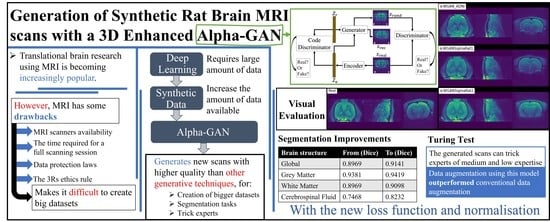
Generation of Synthetic Rat Brain MRI Scans with a 3D Enhanced Alpha Generative Adversarial Network


Abstract
:Featured Application
Abstract
1. Introduction
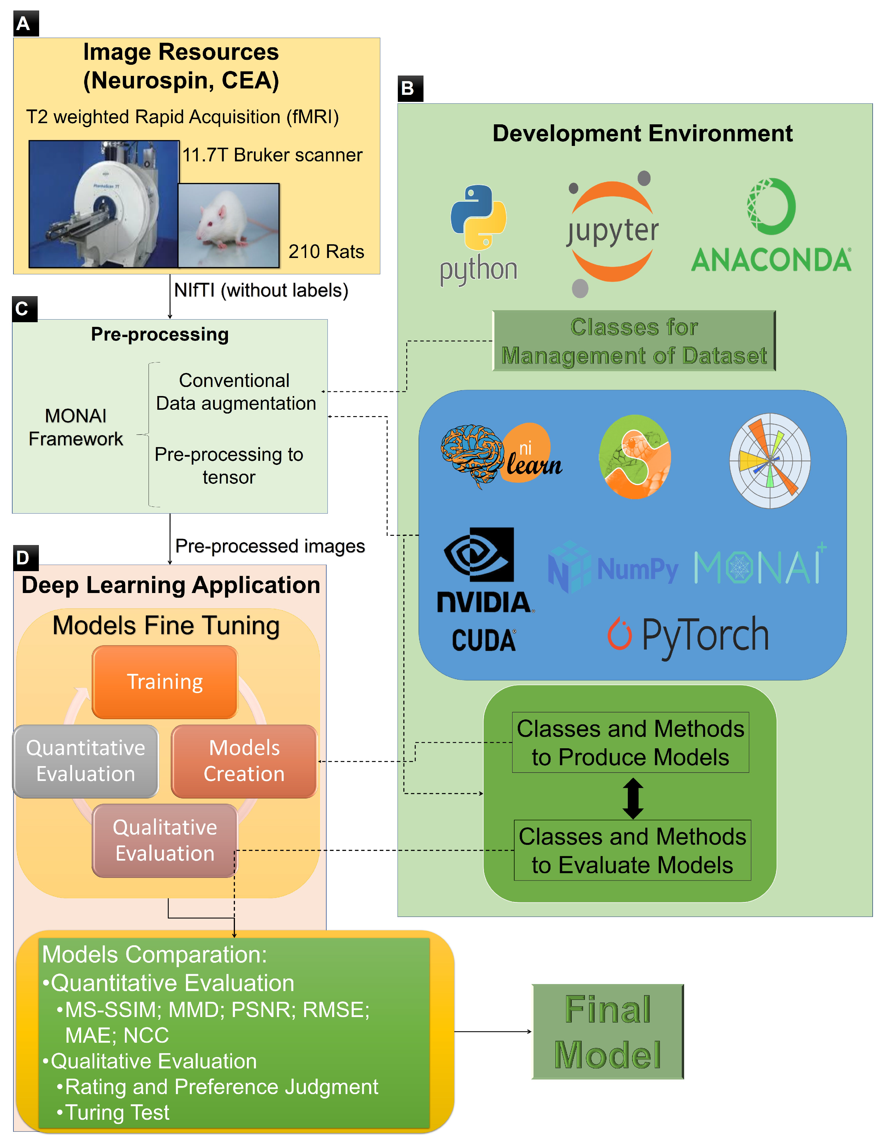
2. Materials and Methods
2.1. Sigma Dataset of Rat Brains
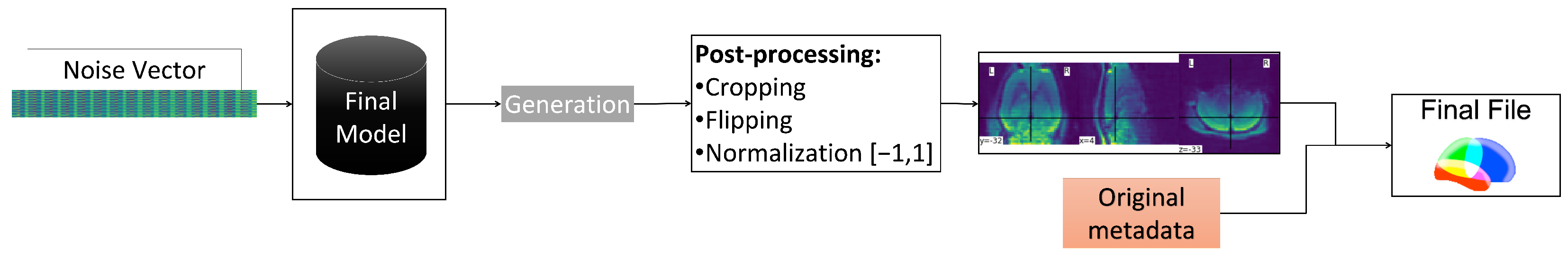
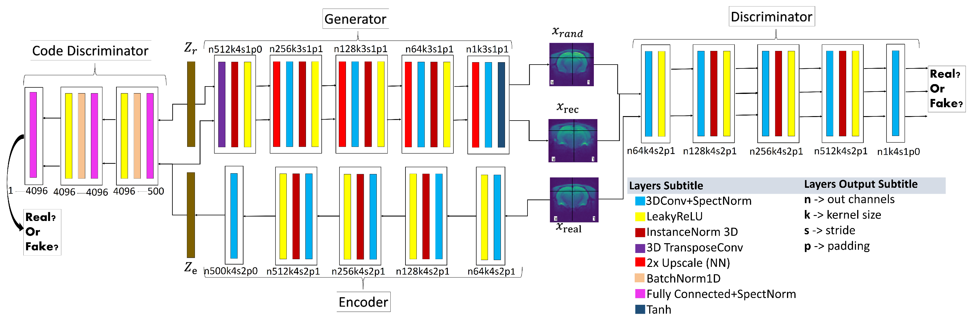
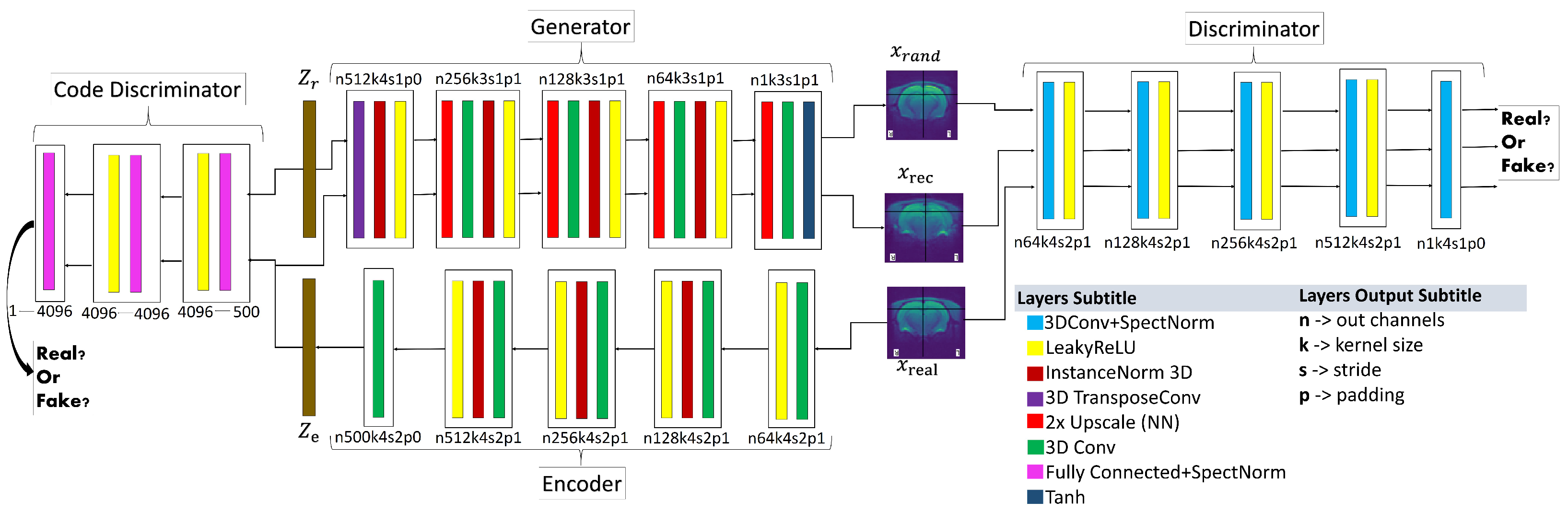
2.2. Overall Process Workflow
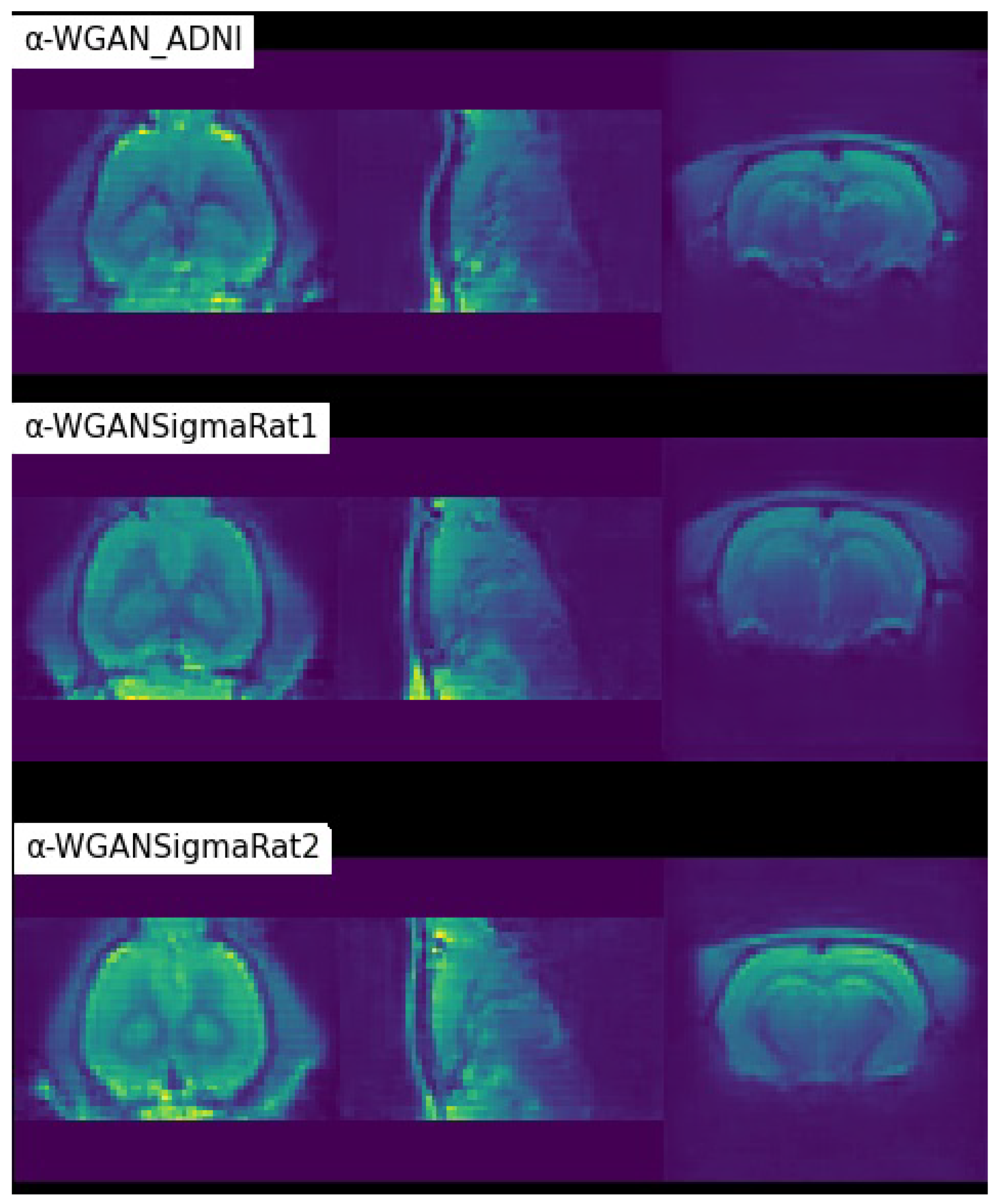
3. Results
4. Discussion
5. Conclusions
Author Contributions
Funding
Institutional Review Board Statement
Informed Consent Statement
Data Availability Statement
Conflicts of Interest
Abbreviations
| CSF | Cerebrospinal Fluid |
| DL | Deep Learning |
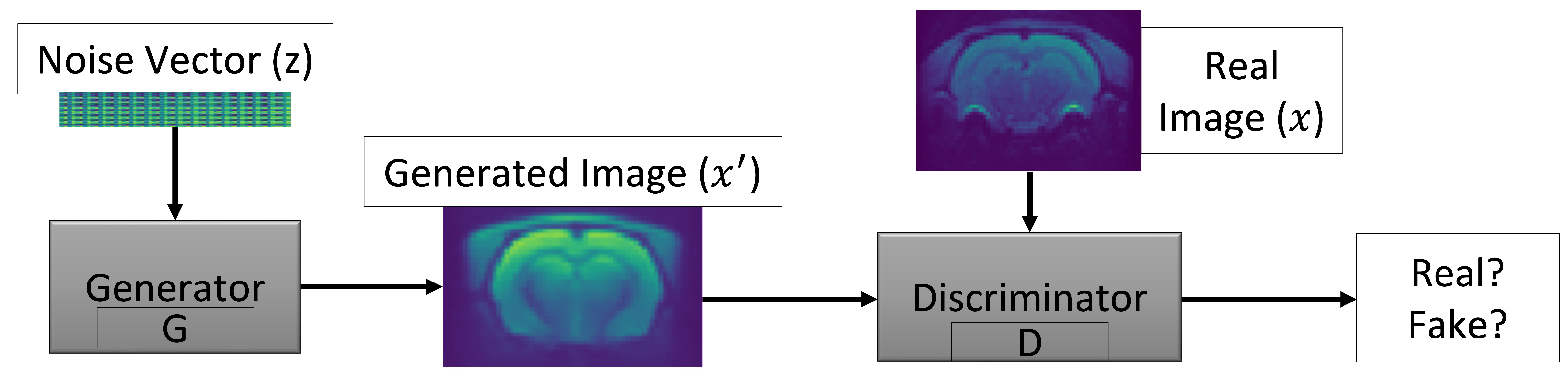
| GAN | Generative Adversarial Networks |
| GDL | Gradient Difference Loss |
| GM | Grey Matter |
| MAE | Mean Absolute Error |
| MMD | Maximum–Mean Discrepancy |
| MRI | Magnetic Resonance Imaging |
| MSE | Mean Squared Error |
| MS-SSIM | Multi-Scale Structural Similarity Index Measure |
| NCC | Normalised Cross Correlation |
| SN | Spectral Normalisation |
| VAE | Variational AutoEncoder |
| WM | White Matter |
References
- Denic, A.; Macura, S.I.; Mishra, P.; Gamez, J.D.; Rodriguez, M.; Pirko, I. MRI in rodent models of brain disorders. Neurotherapeutics 2011, 8, 3–18. [Google Scholar] [CrossRef] [Green Version]
- Brockmann, M.A.; Kemmling, A.; Groden, C. Current issues and perspectives in small rodent magnetic resonance imaging using clinical MRI scanners. Methods 2007, 43, 79–87. [Google Scholar] [CrossRef]
- Barrière, D.A.; Magalhães, R.; Novais, A.; Marques, P.; Selingue, E.; Geffroy, F.; Marques, F.; Cerqueira, J.; Sousa, J.C.; Boumezbeur, F.; et al. The SIGMA rat brain templates and atlases for multimodal MRI data analysis and visualization. Nat. Commun. 2019, 10, 5699. [Google Scholar] [CrossRef] [Green Version]
- Magalhães, R.J.d.S. An Imaging Characterization of the Adaptive and Maladaptive Response to Chronic Stress. Ph.D. Thesis, University of Minho, Braga, Portugal, 2018. [Google Scholar]
- Magalhães, R.; Barrière, D.A.; Novais, A.; Marques, F.; Marques, P.; Cerqueira, J.; Sousa, J.C.; Cachia, A.; Boumezbeur, F.; Bottlaender, M.; et al. The dynamics of stress: A longitudinal MRI study of rat brain structure and connectome. Mol. Psychiatry 2018, 23, 1998–2006. [Google Scholar] [CrossRef]
- Magalhães, R.; Ganz, E.; Rodrigues, M.; Barrière, D.A.; Mériaux, S.; Jay, T.M.; Sousa, N. Biomarkers of resilience and susceptibility in rodent models of stress. In Stress Resilience: Molecular and Behavioral Aspects; Academic Press: Cambridge, MA, USA, 2019; pp. 311–321. [Google Scholar] [CrossRef]
- Boucher, M.; Geffroy, F.; Prévéral, S.; Bellanger, L.; Selingue, E.; Adryanczyk-Perrier, G.; Péan, M.; Lefèvre, C.T.; Pignol, D.; Ginet, N.; et al. Genetically tailored magnetosomes used as MRI probe for molecular imaging of brain tumor. Biomaterials 2017, 121, 167–178. [Google Scholar] [CrossRef]
- Vanhoutte, G.; Dewachter, I.; Borghgraef, P.; Van Leuven, F.; Van Der Linden, A. Noninvasive in vivo MRI detection of neuritic plaques associated with iron in APP[V717I] transgenic mice, a model for Alzheimer’s disease. Magn. Reson. Med. 2005, 53, 607–613. [Google Scholar] [CrossRef]
- Jamgotchian, L.; Vaillant, S.; Selingue, E.; Doerflinger, A.; Belime, A.; Vandamme, M.; Pinna, G.; Ling, W.L.; Gravel, E.; Meriaux, S.; et al. Tumor-targeted superfluorinated micellar probe for sensitive in vivo 19 F-MRI. Nanoscale 2021, 13, 2373–2377. [Google Scholar] [CrossRef]
- Richard, S.; Boucher, M.; Lalatonne, Y.; Mériaux, S.; Motte, L. Iron oxide nanoparticle surface decorated with cRGD peptides for magnetic resonance imaging of brain tumors. Biochim. Biophys. Acta (BBA)-Gen. Subj. 2017, 1861, 1515–1520. [Google Scholar] [CrossRef]
- Foroozandeh, M.; Eklund, A. Synthesizing brain tumor images and annotations by combining progressive growing GAN and SPADE. arXiv 2020, arXiv:2009.05946. [Google Scholar]
- Russell, W.M.S.; Burch, R.L. The Principles of Humane Experimental Technique; Methuen: London, UK, 1959. [Google Scholar]
- Nalepa, J.; Marcinkiewicz, M.; Kawulok, M. Data Augmentation for Brain-Tumor Segmentation: A Review. Front. Comput. Neurosci. 2019, 13, 83. [Google Scholar] [CrossRef] [Green Version]
- Sandfort, V.; Yan, K.; Pickhardt, P.J.; Summers, R.M. Data augmentation using generative adversarial networks (CycleGAN) to improve generalizability in CT segmentation tasks. Sci. Rep. 2019, 9, 16884. [Google Scholar] [CrossRef]
- Motamed, S.; Rogalla, P.; Khalvati, F. Data Augmentation Using Generative Adversarial Networks (GANs) for GAN-Based Detection of Pneumonia and COVID-19 in Chest X-Ray Images. Inform. Med. Unlocked 2020, 27, 100779. [Google Scholar] [CrossRef]
- Mok, T.C.; Chung, A.C. Learning data augmentation for brain tumor segmentation with coarse-to-fine generative adversarial networks. In International MICCAI Brainlesion Workshop; Springer: Cham, Switzerland, 2018; pp. 70–80. [Google Scholar] [CrossRef] [Green Version]
- El-Kaddoury, M.; Mahmoudi, A.; Himmi, M.M. Deep generative models for image generation: A practical comparison between variational autoencoders and generative adversarial networks. In International Conference on Mobile, Secure, and Programmable Networking; Springer: Berlin/Heidelberg, Germany, 2019; pp. 1–8. [Google Scholar]
- Goodfellow, I.J.; Pouget-Abadie, J.; Mirza, M.; Xu, B.; Warde-Farley, D.; Ozair, S.; Courville, A.; Bengio, Y. Generative adversarial nets. Adv. Neural Inf. Process. Syst. 2014, 3, 2672–2680. [Google Scholar]
- Alqahtani, H.; Kavakli-Thorne, M.; Kumar, G. Applications of Generative Adversarial Networks (GANs): An Updated Review. Arch. Comput. Methods Eng. 2019, 28, 525–552. [Google Scholar] [CrossRef]
- Gui, J.; Sun, Z.; Wen, Y.; Tao, D.; Ye, J. A Review on Generative Adversarial Networks: Algorithms, Theory, and Applications. IEEE Trans. Knowl. Data Eng. 2020, 14, 1–28. [Google Scholar] [CrossRef]
- Brock, A.; Donahue, J.; Simonyan, K. Large scale GaN training for high fidelity natural image synthesis. arXiv 2018, arXiv:1809.11096. [Google Scholar]
- Karras, T.; Laine, S.; Aittala, M.; Hellsten, J.; Lehtinen, J.; Aila, T. Analyzing and improving the image quality of stylegan. In Proceedings of the IEEE Computer Society Conference on Computer Vision and Pattern Recognition, Seattle, WA, USA, 13–19 June 2020; pp. 8107–8116. [Google Scholar]
- Shin, H.C.; Tenenholtz, N.A.; Rogers, J.K.; Schwarz, C.G.; Senjem, M.L.; Gunter, J.L.; Andriole, K.P.; Michalski, M. Medical image synthesis for data augmentation and anonymization using generative adversarial networks. In International Workshop on Simulation and Synthesis in Medical Imaging; Springer: Berlin/Heidelberg, Germany, 2018; pp. 1–11. [Google Scholar]
- Paszke, A.; Gross, S.; Massa, F.; Lerer, A.; Bradbury, J.; Chanan, G.; Killeen, T.; Lin, Z.; Gimelshein, N.; Antiga, L.; et al. PyTorch: An Imperative Style, High-Performance Deep Learning Library. In Advances in Neural Information Processing Systems 32; Curran Associates, Inc.: Red Hook, NY, USA, 2019; pp. 8024–8035. [Google Scholar]
- Consortium, T.M. Project MONAI. 2020. Available online: https://zenodo.org/record/4323059#.YXaMajgzaUk (accessed on 25 May 2020).
- Kwon, G.; Han, C.; shik Kim, D. Generation of 3D Brain MRI Using Auto-Encoding Generative Adversarial Networks. In International Conference on Medical Image Computing and Computer-Assisted Intervention; Springer: Cham, Switzerland, 2019; pp. 118–126. [Google Scholar] [CrossRef] [Green Version]
- Kingma, D.P.; Ba, J.L. Adam: A method for stochastic optimization. arXiv 2014, arXiv:1412.6980. [Google Scholar]
- Sun, Y.; Yuan, P.; Sun, Y. MM-GAN: 3D MRI data augmentation for medical image segmentation via generative adversarial networks. In Proceedings of the 11th IEEE International Conference on Knowledge Graph, ICKG 2020, Nanjing, China, 9–11 August 2020; pp. 227–234. [Google Scholar] [CrossRef]
- Miyato, T.; Kataoka, T.; Koyama, M.; Yoshida, Y. Spectral normalization for generative adversarial networks. arXiv 2018, arXiv:1802.05957. [Google Scholar]
- Agrawal, N.; Katna, R. Applications of Computing, Automation and Wireless Systems in Electrical Engineering; Springer: Singapore, 2019; Volume 553, pp. 859–863. [Google Scholar] [CrossRef]
- Mathieu, M.; Couprie, C.; LeCun, Y. Deep multi-scale video prediction beyond mean square error. arXiv 2015, arXiv:1511.05440. [Google Scholar]
- Chen, Y.; Shi, F.; Christodoulou, A.G.; Xie, Y.; Zhou, Z.; Li, D. Efficient and accurate MRI super-resolution using a generative adversarial network and 3D multi-level densely connected network. In International Conference on Medical Image Computing and Computer-Assisted Intervention; Springer: Cham, Switzerland, 2018; pp. 91–99. [Google Scholar] [CrossRef] [Green Version]
- Sánchez, I.; Vilaplana, V. Brain MRI super-resolution using 3D generative adversarial networks. arXiv 2018, arXiv:1812.11440. [Google Scholar]
- Loshchilov, I.; Hutter, F. Decoupled weight decay regularization. arXiv 2017, arXiv:1711.05101. [Google Scholar]
- Borji, A. Pros and Cons of GAN Evaluation Measures: New Developments. Comput. Vis. Image Underst. 2021, 215, 103329. [Google Scholar] [CrossRef]
- Borji, A. Pros and cons of GAN evaluation measures. Comput. Vis. Image Underst. 2019, 179, 41–65. [Google Scholar] [CrossRef] [Green Version]
- Salimans, T.; Goodfellow, I.; Zaremba, W.; Cheung, V.; Radford, A.; Chen, X. Improved techniques for training gans. Adv. Neural Inf. Process. Syst. 2016, 29, 2234–2242. [Google Scholar]
- Rodrigues, M.F. Brain Semantic Segmentation: A DL Approach in Human and Rat MRI Studies. Ph.D. Thesis, Universidade do Minho, Braga, Portugal, 2018. [Google Scholar]
- Penny, W.D.; Friston, K.J.; Ashburner, J.T.; Kiebel, S.J.; Nichols, T.E. Statistical Parametric Mapping: The Analysis of Functional Brain Images; Elsevier: Amsterdam, The Netherlands, 2011. [Google Scholar]


| Operative System | Ubuntu 18.04.3 LTS (64 bits) |
|---|---|
| CPU | Intel Xeon E5-1650 12 Core |
| GPU | GPU – NVIDIA P6000 |
| Cuda Parallel-Processing Cores 3840 | |
| 24 GB GDDR5X | |
| FP32 Performance 12 TFLOPS | |
| Primary Memory | 64 Gb |
| Secondary Memory | 2 Disks of 2 TB |
| 1 Disk of 512 Gb |
| Results | MS-SSIM | NCC ↑ | MAE ↓ | MMD ↓ |
|---|---|---|---|---|
| -WGAN_ADNI [26] | 0.6860 | 0.7241 | 0.0316 | 779.4653 |
| ±0.0066 | ±0.0071 | ±0.0004 | ±27.2016 | |
| -WGANSigmaRat1 | 0.8118 | 0.7887 | 0.0305 | 753.1584 |
| ±0.0051 | ±0.0041 | ±0.0004 | ±24.8816 | |
| -WGANSigmaRat2 | 0.8236 | 0.7527 | 0.0325 | 819.3409 |
| ±0.0056 | ±0.0037 | ±0.0003 | ±20.4437 |
| Rater | ||||||||
|---|---|---|---|---|---|---|---|---|
| 1 High | 2 Low | 3 Medium | 4 Medium | |||||
| Real | Syn | Real | Syn | Real | Syn | Real | Syn | |
| -WGANSigmaRat1 | 1 | 14 | 13 | 2 | 2 | 13 | 5 | 10 |
| -WGANSigmaRat2 | 0 | 15 | 8 | 7 | 4 | 11 | 8 | 7 |
| Real | 19 | 1 | 4 | 16 | 17 | 3 | 12 | 8 |
| Right Answers | 48 | 13 | 41 | 29 | ||||
| Tests | Test1 | Test2 | Test3 | Test4 | Test5 | Test6 | Test7 | Test8 | Test9 |
|---|---|---|---|---|---|---|---|---|---|
| Data sets | Dr174 | Dr174 Ds87 | Dr174 Ds174 | Dr174 Ds261 | Dr174 Ds348 | Ds174 | Ds348 | Dr87 Ds174 | Dr87 Ds348 |
| Global | 0.8969 | 0.9138 | 0.9083 | 0.9078 | 0.9141 | 0.8238 | 0.7646 | 0.8979 | 0.8259 |
| GM | 0.9381 | 0.9419 | 0.9384 | 0.9376 | 0.9412 | 0.8863 | 0.8586 | 0.9316 | 0.8863 |
| WM | 0.8969 | 0.9077 | 0.9037 | 0.9014 | 0.9098 | 0.8202 | 0.7262 | 0.8897 | 0.8301 |
| CSF | 0.7468 | 0.8232 | 0.8098 | 0.8170 | 0.8180 | 0.6095 | 0.4418 | 0.7442 | 0.6273 |
| Tests | Test1 | Test2 | Test5 | Test10 | Test11 | Test12 |
|---|---|---|---|---|---|---|
| Data sets | Dr174 | Dr174 Ds87 | Dr174 Ds348 | Dr174 Da826 | Dr174 Da348 | Dr174 Da348 |
| Global | 0.8969 | 0.9138 | 0.9141 | 0.8183 | 0.8742 | 0.8696 |
| GM | 0.9381 | 0.9419 | 0.9412 | 0.8856 | 0.9214 | 0.9190 |
| WM | 0.8969 | 0.9077 | 0.9098 | 0.7824 | 0.8585 | 0.8501 |
| CSF | 0.7468 | 0.8232 | 0.8180 | 0.6042 | 0.7100 | 0.7018 |
Publisher’s Note: MDPI stays neutral with regard to jurisdictional claims in published maps and institutional affiliations. |
© 2022 by the authors. Licensee MDPI, Basel, Switzerland. This article is an open access article distributed under the terms and conditions of the Creative Commons Attribution (CC BY) license (https://creativecommons.org/licenses/by/4.0/).
Share and Cite
Ferreira, A.; Magalhães, R.; Mériaux, S.; Alves, V. Generation of Synthetic Rat Brain MRI Scans with a 3D Enhanced Alpha Generative Adversarial Network. Appl. Sci. 2022, 12, 4844. https://doi.org/10.3390/app12104844
Ferreira A, Magalhães R, Mériaux S, Alves V. Generation of Synthetic Rat Brain MRI Scans with a 3D Enhanced Alpha Generative Adversarial Network. Applied Sciences. 2022; 12(10):4844. https://doi.org/10.3390/app12104844
Chicago/Turabian StyleFerreira, André, Ricardo Magalhães, Sébastien Mériaux, and Victor Alves. 2022. "Generation of Synthetic Rat Brain MRI Scans with a 3D Enhanced Alpha Generative Adversarial Network" Applied Sciences 12, no. 10: 4844. https://doi.org/10.3390/app12104844
APA StyleFerreira, A., Magalhães, R., Mériaux, S., & Alves, V. (2022). Generation of Synthetic Rat Brain MRI Scans with a 3D Enhanced Alpha Generative Adversarial Network. Applied Sciences, 12(10), 4844. https://doi.org/10.3390/app12104844