Abstract
The kinematic source rupture process of the 2016 Meinong earthquake (Mw = 6.4) in Taiwan was derived from apparent source time functions retrieved from teleseismic S-waves by using a refined homomorphic deconvolution method. The total duration of the rupture process was approximately 15 s, and one slip-concentrated area can be represented as the source model based on images representing static slip distribution. The rupture process began in a down-dip direction from the fault toward Tainan City, strongly suggesting that the rupture had a unilateral northwestern direction. The asperity with an area of approximately 15 × 15 km2 and the maximum slip of approximately 2 m were centered 12.8 km northwest of the hypocenter. Coseismic vertical deformation was calculated based on the source model. Compared with the results derived from InSAR (Interferometric Synthetic Aperture Radar) data, our results demonstrated that the location with maximum uplift was accurately well detected, but our maximum value was just approximately 0.4 times of the InSAR-derived value. It reveals that there are the other mechanisms to affect the vertical deformation, rather than only depending on the source model. At different depths, areas west, east, and north of the hypocenter maintained high values of Coulomb stress changes. This explains the mechanism behind aftershocks being triggered and provides a reference for predicting aftershock locations after a large earthquake. The estimated seismic spectral intensities, including spectral acceleration and velocity intensity (SIa and SIv), were derived. Source directivity effects caused damage to buildings, and we concluded that all damaged buildings were located within a SIa value of 400 gal. Destroyed buildings taller than seven floors were located in an area with a SIv value of 30 cm/s. These observations agree with those on damages caused by the 2010 Jiasian earthquake (ML 6.4) in Tainan, Taiwan.
1. Introduction
1.1. Meinong Earthquake
On 6 February 2016, the Meinong earthquake (ML 6.4) struck southern Taiwan, causing 117 casualties and 551 injuries; as a result of the earthquake, 412 buildings were damaged, some of which collapsed [1]. This infrastructural damage was the most substantial in Taiwan since the 1999 Chi-Chi earthquake. According to the Central Weather Bureau, the epicenter of the Meinong earthquake located at 22.92° N latitude and 120.54° E longitude, and the hypocenter was at a depth of 14.6 km. Notably, the most severe damage was not located near the epicenter of the Meinong earthquake; rather, most damage occurred in the Tainan area, including Tainan City and neighboring districts [2]. Researchers have used various techniques and data to determine the reasons for this damage distribution. It is very valuable to understand the factors that caused serious damages and apply them to disaster managements of the earthquakes that occurred near the densely inhabited districts in western Taiwan.
1.2. Literary Reviews
Lee et al. (2016) [3] first derived a source model through joint inversion. The source model was mainly composed of two asperities, but the main rupture developed in a down-dip direction and then proceeded in the northwest direction. By combining P and depth-phase sP waves recorded at dense arrays through back projection, Jian et al. (2017) [4] revealed that the rupture process was unilateral (northwestward), and the source radiation was modeled as a single asperity with a length of 17 km. By considering ground motion displacement, Kanamori et al. (2017) [5] revealed that the combined effects of crustal structure, rupture directivity, and source slip can amplify seismic waveforms to cause the serious damages in Tainan. By employing a densely distributed seismic network in a seismic array, Lin et al. (2018) [1] derived earthquake rupture processes through finite fault inversion. They indicated that the Meinong earthquake was composed of double source events and that the mainshock source, directivity, and site effects were the main factors causing severe damage to Tainan City. Diao et al. (2018) [2] derived a source model through the joint source inversion of waveforms and geodetic datasets, revealing that rupture directivity may generate large long-period velocity pulses, which were the major factors in the substantial damage to Tainan City. Chen et al. (2019) [6] used the empirical Green function from a small aftershock (ML 4.6) to estimate that the strong motion generation area (SMGA) of the Meinong earthquake was approximately 7.2 × 7.2 km2. They revealed that both the size of SMGA and rise time of the main event followed a self-similar empirical relationship formula derived by Miyake et al. (2003) [7]. By analyzing the aftershock sequence of the Meinong earthquake, Hsu et al. (2020) [8] provided evidence for fluid movement in southwestern Taiwan, concluding that fluids may be a important factor causing deep crustal earthquakes and affecting earthquake hazards. Through the joint inversion of InSAR, Global Positioning System (GPS; 1 Hz), and strong motion data, Yang et al. (2021) [9] inverted the source model of the Meinong earthquake and suggested that this model has a simpler asperity than other models.
On the basis of different methods and recorded data, there are various source models derived to demonstrate some characteristics of the rupturing process when earthquakes are occurring. However, the derived source models had some differences owing to the inversion methods and data used. To detect and understand the source process of an earthquake, Liao et al. (2013) [10] developed the hybrid homomorphic deconvolution (HHD) method to invert the source model of the 1999 Chi-Chi earthquake (Taiwan), obtaining excellent results. They stated that their HHD method can invert and efficiently capture the main characteristics of an earthquake rupture. By employing the same method, Liao and Sheu (2013) [11] inverted the source model of the 2011 Tohoku-Oki earthquake (Japan; Mw 9.0) whose epicentral location could be estimated in advance [12] by means of natural time analysis of Japanese seismicity [13,14] to obtain the source characteristics of that event. Using the aforementioned method, Liao and Huang (2016) [15] derived the source models of two moderate earthquakes (ML 6.2 and 6.0) in 2013 in central Taiwan to calculate the Coulomb stress changes distributed around central Taiwan and predict potential earthquake locations. The aim of this study was to use HHD to invert a source model of the Meinong earthquake and employ the inverted model to calculate surface deformation and Coulomb stress changes at different depths and estimate seismic spectral intensities SIa and SIv. Finally, we compare our results with other results in the literature to determine the validity of our inverted model as an alternative approach to source inversion.
2. Materials and Methods
2.1. Hybrid Homomorphic Deconvolution
Observed seismic data can be modeled mathematically as a convolution
where is Green’s function, is the seismic source time function (STF), and represents the convolution operation. The complex cepstrum of a seismogram X(t) is defined as follows [16] (Li and Nabelek, 1999):
The inverse transform is defined as follows:
The series in the complex cepstrum is real, and the complex cepstrum domain is called the quefrency domain [17]. A indicated in (2) and (3), the cepstrum of a seismogram is the sum of the cepstra of its convolutional components; that is,
According to previous studies [16,18], the STF tends to occupy low quefrency regions, whereas the Green function with a rapidly varying spectrum occupies a high quefrency region. The STF is expected to be concentrated near t = 0 in the quefrency domain, and structural responses are assigned to a high quefrency region. Therefore, for recovering and , the first step is to apply linear filtering to cepstrum for separating and . The second step involves taking the inverse transform of them such that the corresponding convolutional components and of the seismogram X(t) can be separated. However, the phase unwrapping problem may occur in the inverse transform, as in (2), owing to the log operation in the cepstrum. To improve the phase unwrapping computation of the signal , we use a method proposed by Sitton et al. (2003) [19] based on polynomial factoring algorithms. If is calculated, we can further modify with the constraints proposed by Bertero et al. (1997) [20], including nonnegativity, causality, and finite duration, to fit the physical meanings of STFs. To avoid amplitude differences due to the radiation patterns of earthquake events, we imposed a constraint on , which denotes one earthquake STF estimated at i-th station must have the same seismic moment as that at all stations.
2.2. Source Inversion
An observed STF at i-th station, , can be represented as the summation of all the weighted STFs at subfault , with the time delay due to wave propagation and the propagation of the rupture front with respect to the hypocenter taken into account.
where is the time delay due to the wave and rupture propagation, i is a station index, j is a subfault index, and is the slip weight of each subfault. Equation (5) can be written in matrix form:
where S is a data matrix consisting of observed STFs, D is an unknown vector composed of the slip weight of each subfault, and K is the matrix determined by each STF of subfault associated with the aforementioned time delay. If we solve (6) to obtain , then the slip amplitudes at each subfault, , can be obtained as follows:
where A is the subfault area, is the seismic moment, and μ is the shear modulus. A constraint condition, , must be imposed on (6) to solve . Finally, we can estimate by applying the least square and conjugate gradient methods [21] to obtain the slip source model.
2.3. Coulomb’ Stress Changes
Under the assumption that a material is isotropic and elastic, the stress tensor sij at one spatial point in the material can be calculated using the source model of one large earthquake.
where are the components of the identity matrix, are strain tensors, and and are Lamé parameters. The Coulomb stress change, ∆CFS, on the target failure plane is represented as [22] follows:
where is the shear stress change on the receiver plane, is the change in normal stress, and μ′ is the effective coefficient of friction. and can be calculated as follows:
where and are the normal and shear slip vectors, respectively. We assumed that the shear modulus was Pa, the Poisson ratio was 0.25, and the value was 0.4. On the basis of the physical meaning of ∆CFS, increased Coulomb stress represents loading stress, pushing the fault toward brittle failure; conversely, decreased Coulomb stress represents unloading stress, inhibiting earthquake rupture.
2.4. SSIs
In a seismic recording, spectral acceleration, velocity, and displacement are denoted as , , and respectively, where T and are period and damping, respectively. On the basis of the corresponding spectral acceleration (SIa), velocity (SIv), and displacement (SId), the SIs are defined as follows:
where parameters are dependent on earthquake size and building height. The empirical formula applied for estimating the natural period of a building is as follows:
where is a constant (0.05 < < 0.085) and is the height of a building in meters. A typical story height in Taiwan is approximately 2.5 to 3 m; accordingly, Martinez-Rueda (1998) [23] suggested that parameters in (12)–(14) should be assumed to be 0.1, 0.6, 0.6, 1.6, 1.6, and 3 s, respectively. According to (15), the different integration ranges in (12)–(14) correlate to buildings with 1–6 floors, 7–22 floors, and >22 floors, respectively.
3. Results and Discussion
3.1. Source Model
The H(t) value retrieved from the seismogram data recorded at one station is called the apparent SFT (ASTF). ASTFs from different stations represent the energy release process of an earthquake from different distances and directions. If the ASTFs are retrieved from stations well distributed around the hypocenter of an earthquake, they will be employed to invert the rupture process by Equations (5)–(7). We examined data from 16 stations to determine the ASTFs (recorded by Incorporated Research Institutions Seismology, IRIS) around the hypocenter of the Meinong earthquake, as presented in Figure 1.
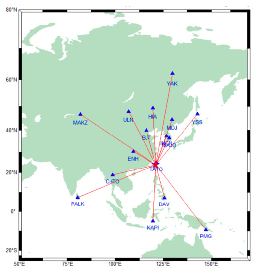
Figure 1.
Locations of the epicenter (star) of the Meinong earthquake and 16 teleseismic stations (triangles) used for assessing the STFs of the event (Mw = 6.4).
For seismic data, the secondary seismic waves (S-waves) of vertical components were used. The S-wave displacements (solid line) filtered by a band-pass filter with a frequency band of 0.001–1 Hz are displayed in Figure 2.
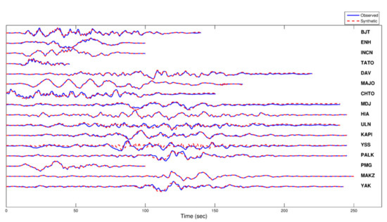
Figure 2.
Comparisons of the observed S-wave waveforms (blue line) and synthetic waveforms (dashed line) for the Meinong earthquake. The synthetic waveforms are the convolutions of the derived ASTFs obtained using HHD, with Green’s functions extracted from the waveforms.
That figure presents a comparison of observed (solid line) and predicted (red line) S-waves, as determined by the convolution of estimated Green’s functions with the ASTFs of stations. The observed and predicted S-waves were similar. We derived the ASTFs from the HHD of S-waves recorded at the stations indicated in Figure 1. On the basis of the ASTFs (blue line) in Figure 3, the rupture duration was estimated to be 15 s, and the main moment may have occurred in the first 7 s and decreased after 7 s.
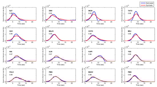
Figure 3.
Comparison of ASTFs (blue line) for the Meinong event calculated using the proposed method for handling teleseismic data and ASTFs (red line) calculated using the inverted source model. The correlation coefficients between the estimated and synthetic ASTFs were all above 0.94.
Jian et al. (2017) [4] used the back projection method and examined the seismic waves recorded by two arrays, proposing that energy release in the source process of the Meinong earthquake lasted approximately 7 s. Lee et al. (2016) [3] proposed that the duration time of STF of the Meinong earthquake was 16 s and that the source model of this event comprised two main asperities. The main energy higher than 60% of the total moment was released in the first 8 s. The STF curve of that Meinong event derived by [2] also indicated that the source duration was 12 s and the main energy of the Meinong earthquake was estimated to have been released in the first 6 s. Our result is generally consistent with those of relevant studies.
On the basis of source duration, we determine that the fault model was composed of a single plane and that the fault dimension was approximately 45 × 39 km2, with the epicenter located at a depth of 14.6 km. For source model inversion, the fault was further divided into subfaults of equal size (3 × 2.6 km2). The frequency band of 0.001–1 Hz reveals the minimum waveform period (1 s), and the crustal S-wave velocity of an earthquake with a focal depth of 14.6 km is approximately 4.6 km/s; therefore, the minimum wavelength was 4.6 km. According to [24], the resolving length is λ/4; the resolving length in this study was determined to be approximately 1.15 km smaller than 4.6 km, ensuring that the inverted source model was reasonable and had a suitable resolution. Figure 4 presents a map view of slip amplitude distributions, where the red star is the epicenter of the Meinong event.
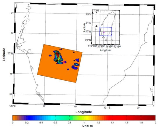
Figure 4.
Slip distribution on the indicated fault derived using the source inversion technique. The maximum slip value was approximately 2.4 m. The star represents the epicenter of the Meinong earthquake.
Figure 4 reveals that the rupture direction was northwest; this finding agrees with the results of [3,4,9]. In addition, the finding that the maximum slip was located approximately at the position with longitude of 120.4° E and attitude of 23° N was consistent with the inverted source model [2,3,4,9]. Figure 5 demonstrates the slip amplitude distribution on the fault.
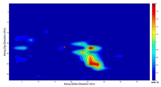
Figure 5.
Slip distribution on the indicated fault with distance used as a reference.
From the inverted model results, the rupture process can be modeled as a large asperity with an area of approximately 15 × 15 km2, and the maximum slip was 2 m. The asperity located below the hypocenter and the high slip area was at a depth of approximately 14–18 km, suggesting that the main rupture consisted of strike slips and down-dip slips propagating from the hypocenter in the northwest direction.
3.2. Application
3.2.1. Vertical Surface Deformation
On the basis of our inverted source model, we used a method proposed by Okada (1992) [25] to calculate the surface uplift (Figure 6) and compare it with the corresponding InSAR results by Mai et al. (2021) [26].
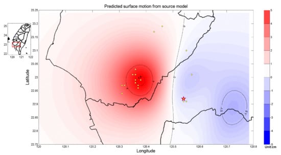
Figure 6.
Predicted vertical surface displacements calculated using the proposed inverted model. The red star is the hypocenter, and the small yellow points represent aftershocks. Areas with high displacement values located northwest of the hypocenter indicate that the fault rupture extended from the hypocenter in the northwest direction along the seismogenic fault.
The major vertical displacements presented in Figure 6 were seemingly centered northwest of the Meinong earthquake’s hypocenter. According to [8], this indicates that the fault rupture extended from the hypocenter in the northwest direction along the seismogenic fault. Compared with the results derived from InSAR data, our results could better detect areas with high vertical displacement values, but our derived maximum vertical displacement result was 5 cm, which is smaller than the maximum displacement result derived using InSAR data (13 cm). Mai et al. (2021) [26] used the source model of [3] to calculate surface vertical displacement. They obtained a maximum surface displacement of approximately 5 cm, and the areas corresponding to high values were slightly farther west compared with observations from InSAR data-derived results. According to [26], rather than only coseismic fault slip, some other mechanisms may underlie the surface pop-up. Yang et al. (2021) [9] offered clear explanations of such mechanisms, including responses of aftershocks in soil liquefaction areas and activities associated with the Xinhua fault by the Meinong event. In this study, the earthquake model was assumed to be a half-space one, as in the study of [25], and differences between estimated and observed surface deformations were expected; surface deformation was affected by the local geologic properties. Therefore, the calculated results based on the source model can provide a valuable reference for investigating the factors contributing to actual observations.
3.2.2. Coulomb Stress Changes
Coulomb stress changes trigger aftershocks and successive earthquakes when a large earthquake occurs. Ganas et al. (2012) [27] stated that an earthquake on a fault plane can trigger subsequent earthquakes at short distances from its hypocenter through Coulomb stress transformation. Previous studies [28,29] had suggested that aftershocks can occur in areas with a high static ΔCFS value and indicated that a location with a positive ΔCFS could increase loading stress to make faults more susceptible to brittle failure. When the ΔCFS is greater than 0.1 bar in some areas, subsequent earthquakes may occur in such areas ([30,31]). On the basis of results from related studies, we calculated the ΔCFS of the Meinong earthquake based on the inverted model to investigate the activities of aftershocks and determine the potential for subsequent earthquakes. In this study, Okada’s method (1992) [25] was applied to calculate ΔCFSs at different depths, and the results are presented in Figure 7.

Figure 7.
Coulomb stress change (ΔCFS) distributions at different depths (10–30 km). The star represents the hypocenter, and the yellow dots represent aftershocks. Areas with high ΔCFS values were west, east, and north of the hypocenter. Coupled with aftershock activities, the ΔCFS value could be used to explain the mainshock–aftershock relationship and the earthquake’s aftershock triggering mechanism.
Three areas presented in Figure 7 are worthy of discussion. At depths below 20 km, some high ΔCFS values of >0.1 bar gradually accumulated and formed a patch around the area at a longitude of 120.3° E to 120.4° E and latitude of 22.85° N to 23.1° N to the west of the hypocenter. Coincidentally, a cluster of aftershocks with depths of 22 to 30 km was located in this area. These aftershocks may be triggered by the mainshock, offering strong evidence that our derived result is meaningful and fits well with findings on the triggering mechanism. The second area located north of the hypocenter, with high ΔCFS values of >0.1 bar, had a depth of 10–25 km, and some aftershocks were triggered here. Wen et al. (2017) [32] suggested that a fault of northwest-to-southeast trend existed and that a north-dipping fault located north of the source area may have moved, affected by the initial shock. This suggestion agreed with our derived results. The third area within a longitude of 120.55° E to 120.65° E and latitude of 22.85° N to 23° N was located east of the hypocenter and formed a path with high ΔCFS values (>0.1 bar) from depths of 10–25 km. Jian et al. (2017) [4] demonstrated that aftershocks occurred within 10 days of the main shock and that the background seismicity was >2.0 ML. They also revealed that the area confined to a longitude of 120.5° E to 120.65° E and latitude of 22.85° N to 22.95° N had a cluster of aftershocks distributed at depths between 10 and 20 km. According to previous results, our derived ΔCFS pattern seems to estimate the distributions of aftershocks successfully, indicating that our inverted source model is highly accurate.
3.2.3. SSIs
Liao et al. (2020) [33] applied SSIs, including SIa, SIv, and SId defined in Equation (12), Equation (13) and Equation (14), respectively, to estimate damage to buildings caused by the potential earthquake in central Taiwan and revealed that these indexes are highly useful for evaluating damage to buildings. Accordingly, we simulated strong near-field motions in the broadband range using the method proposed by Joshi et al. (2015) [34] and calculated the SIs distributed around Tainan to offer a reference for disaster management. Because no building taller than 22 floors was damaged by the Meinong event in Tainan, we did not calculate Sid values. As previously stated, SIa and SIv values were used to estimate damage to buildings with 1–7 and 7–22 floors, respectively. The simulated SIa and SIv distributions are presented in Figure 8 and Figure 9, respectively.
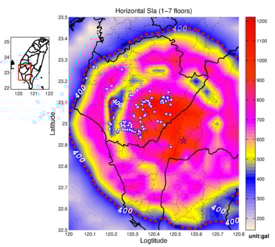
Figure 8.
SIa distribution calculated using the inverted source model. The dashed line indicates areas with an SIa value of 400 gal; damaged buildings with 1–6 floors were located within the contour line. The red star represents the hypocenter of the Meinong earthquake, and the white squares represent the buildings damaged by this earthquake [36].
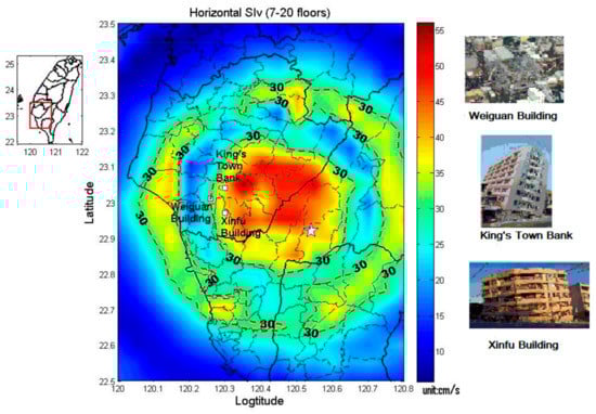
Figure 9.
SIv distribution calculated using the inverted source model. The dashed line indicates areas with an SIv value of 30 cm/s; damaged buildings taller than 7 floors were located within the contour line.
High SIa values of >900 gal and high SIv values of >45 cm/s were observed northwest of the hypocenter, revealing that source effects and rupture directivity markedly influenced the SI values and extent of damages to buildings. As indicated in Figure 8, most of the damaged buildings (represented by white squares) were in the region with SIa values higher than 700 gal and distributed along the northwest of the hypocenter. Evidently, rupture directivity can severely damage buildings. Related studies ([1,3,9]) have demonstrated that directivity effects are among the main factors causing damage to buildings. All damaged buildings were located within the contour line of 400 gal, which is consistent to the findings of Yeh and Peng (2012) [35]. From an investigation of the Jiasian earthquake (ML = 6.4), Yeh and Peng (2012) [35] revealed that damaged buildings were located in areas with SIa values higher than 400 gal and SIv values higher than 30 cm/s. Figure 9 reveals that three damaged buildings were taller than seven floors, and all were located within the area enclosed by the contour line of 30 cm/s. Earthquake-induced resonance effects may be an important factor contributing to severe infrastructural damage.
4. Discussion and Conclusions
In this study, we used HHD to invert the source model of the Meinong earthquake. Our inverted model is similar to the source model of [9]. One major asperity was modeled as a source process, and the location of the asperity relative to the epicenter and the rupture direction (northwest) was fairly consistent. The source process was also modeled as an asperity by [2]; however, their study differed in that their slip direction was west-northwest. Because of differences in the data and inversion methods used, a second small asperity at a depth of 15 km in the study of [3] was not detected in our model. We applied the inverted source in this study to compute the vertical surface deformation, Coulomb stress change, and SSIs to compare them with the corresponding values in previous studies in order to determine our model’s validity. Areas with high surface vertical displacement values were northwest of Meinong’s hypocenter, indicating that the rupture direction was northwest. Under the influence of various geological properties and other fault activities, our estimated maximum value of surface vertical displacements was 5 cm, which was an underestimate (the InSAR-derived maximum value was 13 cm). However, areas with high values were accurately detected by our source model. The derived ΔCFS values indicated that three areas had particularly high values; these areas were east, west, and north of the hypocenter. Aftershocks with depths of 10–25 km were clustered in the eastern and western areas, and such aftershocks may have contributed to be triggered by ΔCFS. The high positive ΔCFS values that occurred north of the hypocenter may have affected both movement with a northwest-to-southeast trend and north-dipping blind fault, and aftershocks. Finally, we computed SIa and SIv to evaluate damage to two groups of buildings (1–7 and 7–22 floors). According to the distribution of SI values, the damaged buildings were located northwest of the hypocenter, indicating that source directivity may have been a key factor behind this building damage. All damaged buildings with 1–7 floors were located in an area with SIa greater than 400 gal, and the damaged buildings with 7–22 floors were in the area with SIv greater than 30 cm/s, respectively; these observations are consistent with those related to the Jiasian earthquake. These results were derived using our inverted source model, proving the validity of this inverted model and the effectiveness of the HHD method.
Author Contributions
Conceptualization, B.-Y.L. and H.-C.H.; methodology, B.-Y.L.; software, B.-Y.L.; validation, B.-Y.L., H.-C.H. and S.X.; formal analysis, B.-Y.L.; investigation, B.-Y.L.; resources, B.-Y.L.; data curation, B.-Y.L.; writing—original draft preparation, H.-C.H.; writing—review and editing, H.-C.H.; visualization, B.-Y.L.; supervision, H.-C.H.; project administration, S.X.; funding acquisition, S.X. All authors have read and agreed to the published version of the manuscript.
Funding
This research was funded by Krirk University, Bangkok, Thailand.
Institutional Review Board Statement
Not applicable.
Informed Consent Statement
Not applicable.
Data Availability Statement
Not applicable.
Conflicts of Interest
The authors declare no conflict of interest.
References
- Lin, Y.Y.; Yeh, T.Y.; Ma, K.F.; Song, A.T.R.; Lee, S.J.; Huang, B.S.; Wu, Y.M. Source characteristics of the 2016 Meinong (ML 6.6), Taiwan, earthquake, revealed from dense seismic arrays: Double sources and pulse-like velocity ground motion. Bull. Seismol. Soc. Am. 2018, 108, 188–199. [Google Scholar] [CrossRef]
- Diao, H.; Kobayashi, H.; Koketsu, K. Rupture process of the 2016 Meinong, Taiwan, earthquakeandits effects on strong ground motions. Bull. Seismol. Soc. Am. 2018, 108, 163–174. [Google Scholar] [CrossRef]
- Lee, S.J.; Yeh, T.Y.; Lin, Y.Y. Anomalously large ground motion in the 2016 ML 6.6 Meinong, Tai¬wan, earthquake: A synergy effect of source rupture and site amplification. Seismol. Res. Lett. 2016, 87, 1319–1326. [Google Scholar] [CrossRef]
- Jian, P.R.; Hung, S.H.; Meng, L.; Sun, D. Rupture characteristics of the 2016 Meinong earthquake revealed by the back projection and directivity analysis of teleseismic broadband waveforms. Geophys. Res. Lett. 2017, 44, 3545–3553. [Google Scholar] [CrossRef]
- Kanamori, H.; Ye, L.; Huang, B.S.; Huang, H.H.; Lee, S.J.; Liang, W.T.; Lin, Y.Y.; Ma, K.F.; Wu, Y.M.; Yeh, T.Y. A strong-motion hot spot of the 2016 Meinong, Taiwan, earthquake (Mw = 6.4). Terr. Atmos. Ocean. Sci. 2017, 28, 637–650. [Google Scholar] [CrossRef][Green Version]
- Chen, Y.C.; Huang, H.C.; Iwata, T.; Asano, K. Strong ground motion simulation of 2016 ML6.6 Meinong, Taiwan, earthquake using the empirical Green’s function method. J. Geophys. Res. Solid Earth 2019, 124, 12905–12919. [Google Scholar] [CrossRef]
- Miyake, H.; Iwata, T.; Irikura, K. Source characterization for broadband ground-motion simulation: Kinematic heterogeneous source model and strong motion generation area. Bull. Seismol. Soc. Am. 2003, 93, 2531–2545. [Google Scholar] [CrossRef]
- Hsu, Y.F.; Huang, H.H.; Huang, M.H.; Tsai, V.C.; Chuang, R.Y.; Feng, K.F.; Lin, S.H. Evidence for fluid migration during the 2016 Meinong Taiwan, aftershock sequence. J. Geophys. Res. 2020, 125, e2020JB019994. [Google Scholar] [CrossRef]
- Yang, Y.H.; Chen, Q.; Diao, X.; Zhao, J.J.; Xu, L.; Hu, J.C. New interpretation of the rupture process of the 2016 Taiwan Meinong Mw 6.4 earthquake based on the InSAR, 1-Hz GPS and strong motion data. J. Geod. 2021, 95, 121. [Google Scholar] [CrossRef]
- Liao, B.Y.; Yeh, Y.T.; Sheu, T.W.; Huang, H.C.; Yang, L.S. A rupture model for the 1999 Chi-Chi earthquake from inversion of teleseismic data using the hybrid homomorphic deconvolution method. Pure Appl. Geophys. 2013, 170, 391–407. [Google Scholar] [CrossRef]
- Liao, B.Y.; Sheu, T.W. Slip distribution of the Tohoku-Oki earthquake (Mw 9.0) inferred from the refined homomorphic deconvolution method. J. Asian Earth Sci. 2013, 73, 263–273. [Google Scholar] [CrossRef]
- Sarlis, N.V.; Skordas, E.S.; Varotsos, P.A.; Nagao, T.; Kamogama, M. Spatiotemporal variations of seismicity before major earthquakes in the Japanese area and their relation with the epicentral locations. Proc. Natl. Acad. Sci. USA 2015, 112, 986–989. [Google Scholar] [CrossRef] [PubMed]
- Sarlis, N.V.; Skordas, E.S.; Varotsos, P.A. Order parameter fluctuations of seismicity in natural time before and after mainshocks. Europhys. Lett. (EPL) 2010, 91, 59001. [Google Scholar] [CrossRef]
- Varotsos, P.A.; Sarlis, N.V.; Skordas, E.S. Study of the temporal correlations in the magnitude time series before major earthquakes in Japan. J. Geophys. Res. Space Phys. 2014, 119, 9192–9206. [Google Scholar] [CrossRef]
- Liao, B.Y.; Huang, H.C. Coulomb stress changes and seismicity in central Taiwan due to the Nantou blind-thrust earthquakes in 2013. J. Asian Earth Sci. 2016, 124, 169–180. [Google Scholar] [CrossRef]
- Li, X.Q.; Nabelek, J.L. Deconvolution of teleseismic body waves for enhancing structure beneath a seismometer array. Bull. Seismol. Soc. Am. 1999, 89, 190–201. [Google Scholar]
- Oppenheim, A.V.; Schafer, R.W. From frequency to quefrency: A history of the cepstrum. IEEE Signal Process. Mag. 2004, 21, 95–106. [Google Scholar] [CrossRef]
- Jin, D.J.; Eisner, E. A review of homomorphic deconvolution. Rev. Geophys. 1984, 22, 255–263. [Google Scholar] [CrossRef]
- Sitton, G.A.; Burrus, C.S.; Fox, J.W.; Treitel, S. Factoring very-high-degree polynomials. IEEE Signal Process. Mag. 2003, 20, 27–42. [Google Scholar] [CrossRef]
- Bertero, M.; Bindi, D.; Boccacci, P.; Cattaneo, M.; Eva, C.; Lanza, V. Application of the projected Landweber method to the estimation of the source time function in seismology. Inverse Probl. 1997, 13, 456–486. [Google Scholar] [CrossRef]
- Ward, D.; Barrientos, S.E. An inversion for slip distribution and fault shape from geodetic observations of the 1983, Borah Park, Idaho, earthquake. J. Geophys. Res. Solid Earth 1986, 91, 4909–4919. [Google Scholar] [CrossRef]
- Ganas, A.; Gosar, A.; Drakatos, G. Static stress changes due to the 1998 and2004 Krn Mountain (Slovenia) earthquakes and implications for futureseismicity. Nat. Haz. Earth Syst. Sci. 2008, 8, 59–66. [Google Scholar] [CrossRef]
- Martinez-Rueda, J.E. Scaling procedure for natural accelerograms based on a system of spectrum intensity scales. Earthq. Spectra 1998, 14, 135–152. [Google Scholar] [CrossRef]
- Zhou, Y.H.; Xu, L.S.; Chen, Y.T. Source process of the 4 June 2000 southern Sumatra, Indonesia, earthquake. Bull. Seismol. Soc. Am. 2002, 92, 2027–2035. [Google Scholar] [CrossRef]
- Okada, Y. Internal deformation due to shear and tensile faults in a half-space. Bull. Seismol. Soc. Am. 1992, 82, 1018–1040. [Google Scholar] [CrossRef]
- Mai, H.A.; Lee, J.C.; Chen, K.H.; Wen, K.L. Coulomb stress changes triggering surface pop-up during the 2016 Mw 6.4 Meinong earthquake with implications for earthquake-induced mud diapiring in sw Taiwan. J. Asian Earth Sci. 2021, 108, 104847. [Google Scholar] [CrossRef]
- Ganas, A.; Roumelioti, Z.; Chousianitis, K. Static stress transfer from the May20, 2012, M 6.1 Emilia-Romagna (northern Italy) earthquake using a co-seismic slip distribution model. Ann. Geophys. 2012, 55, 655–662. [Google Scholar]
- Hardebeck, J.L.; Nazareth, J.J.; Hauksson, E. The static stress change triggering model: Constraints from two southern California aftershocks sequences. J. Geophys. Res. 1998, 103, 427–437. [Google Scholar] [CrossRef]
- Sarkarinejad, K.; Ansari, S. The Coulomb stress changes and seismicity rate due to the 1990 Mw 7.3 Rudbar earthquake. Bull. Seismol. Soc. Am. 2014, 104, 2943–2952. [Google Scholar] [CrossRef]
- Harris, R.A.; Simpson, R.W.; Reseanberg, P.A. Influence of static stress changes on earthquake locations in southern California. Nature 1995, 375, 221–224. [Google Scholar] [CrossRef]
- Harris, R.A.; Simpson, R.W. Suppression of large earthquakes by stress shadows: A comparison of Coulomb and rate-and-state failure. J. Geophys. Res. 1998, 103, 24439–24451. [Google Scholar] [CrossRef]
- Wen, S.; Yeh, Y.L.; Chang, Y.Z.; Chen, C.H. The seismogenic process of the 2016 Meinong earthquake, southwest Taiwan. Terr. Atmos. Ocean. Sci. 2017, 28, 651–662. [Google Scholar] [CrossRef]
- Liao, B.Y.; Liu, C.N.; Sheu, T.W.; Yeh, Y.T. Earthquake Hazard in Central Taiwan Evaluated Using the Potentially Successive 2013 Nantou Taiwan Earthquake Sequences. Geomat. Nat. Hazards Risk 2020, 11, 678–697. [Google Scholar] [CrossRef]
- Joshi, A.; Kuo, C.; Dhibar, H.; Sandeep, P.; Sharma, M.L.; Wen, K.L.; Lin, C.M. Simulation of the records of the 27 March 2013 Nantou Taiwan earthquake using modified semi-empirical approach. Nat. Hazards 2015, 78, 995–1020. [Google Scholar] [CrossRef]
- Yeh, Y.T.; Peng, W.F. A Survey of Factors that Cause Damages by Moderate-Sized Earthquakein Central Taiwan Research Report on the Results of the Central Weather Bureau; Cheng Kung University: Tainan, Taiwan, 2012; No.MOTC-CWB-101-E-10. [Google Scholar]
- Data on Damaged Building by Meinong Earthquake. Available online: https://data.tainan.gov.tw/dataset/0206-earthquake/resource/476c935a-1611-40f0-ae46-0b53fd588c1f (accessed on 12 November 2021).
Publisher’s Note: MDPI stays neutral with regard to jurisdictional claims in published maps and institutional affiliations. |
© 2022 by the authors. Licensee MDPI, Basel, Switzerland. This article is an open access article distributed under the terms and conditions of the Creative Commons Attribution (CC BY) license (https://creativecommons.org/licenses/by/4.0/).