Article

Influences of High-Speed Train Speed on Tunnel Aerodynamic Pressures

Key Laboratory of Urban Underground Engineering of Ministry of Education, Beijing Jiaotong University, Beijing 100044, China
*
Author to whom correspondence should be addressed.
Appl. Sci. 2022, 12(1), 303; https://doi.org/10.3390/app12010303
Submission received: 1 December 2021 / Revised: 22 December 2021 / Accepted: 26 December 2021 / Published: 29 December 2021
(This article belongs to the Special Issue Deep Rock Mass Engineering: Excavation, Monitoring, and Control)

Abstract

:
To comprehensively investigate the characteristics of aerodynamic pressures on a tunnel caused by the whole tunnel passage of a high-speed train at different speeds, we conduct a series of three-dimensional numerical simulations. Based on the field test results obtained by other researchers, the input parameters of our numerical simulation are determined. The process of a high-speed train travelling through a railway tunnel is divided into three stages according to the spatial relationship between the train and tunnel. Stage I: before train nose enters the entrance; Stage II: while the train body runs inside the tunnel; Stage III: after the train tail leaves the exit. The influences of high-speed train speed on the tunnel aerodynamic pressures of these three stages are systematically investigated. The results show that the maximum peak pressure value decreases with increasing distance from the entrance and increases with increasing train speed in Stage I. There is an approximately linear relationship between the three types of maximum peak pressure (positive peak, negative peak, and peak-to-peak pressures) and the power of the train speed in Stage II. These three types of maximum peak pressure values of the points near tunnel portals increase with increasing train speed in Stage III. Moreover, these three types of maximum peak pressure in the tunnel’s middle section at different train speeds are more complex than those near the tunnel portals, and there is one or more turning points due to the superimposed effects of different pressure waves.

1. Introduction

After a high-speed train travels through a railway tunnel, the aerodynamic pressure waves are generated and exert loads on the tunnel lining. The interactions between the running train and the air inside the tunnel produce pressure waves that propagate along the tunnel at the speed of sound. Moreover, the pressure field surrounding the running train also exerts pressure on tunnel lining at the same speed of train [1]. The pressure waves are partially reflected at tunnel portals and other discontinuities, the interactions of which produce a complex pressure field on tunnel [2,3,4,5,6]. The adverse effects associated with the aerodynamic pressures increase with increasing train speed, because of the approximately linear relationship between the amplitude of pressure change and the square of train speed [7]. For example, the aerodynamic fatigue damage of tunnel lining under long-term cycles of aerodynamic pressures [8]. Therefore, the research on the influence of train speed on tunnel aerodynamic pressures has a practical significance for tunnel structural safety during operation.
The aerodynamic pressures associated with a high-speed railway (HSR) tunnel have been investigated by field test, moving model rig, theoretical analysis, and numerical simulation. The related studies mainly focus on the train speed, train marshalling form, train nose length, tunnel length, tunnel hood configuration, and blockage ratio. Using the field test, the influences of train speed and marshalling form on tunnel aerodynamic pressures were investigated [9,10]. Adopting the moving model rig, the effects of tunnel hood configuration and train speed on tunnel aerodynamic pressures were studied [11,12]. Employing the theoretical analysis, the influences of hood configuration and Mach number on initial aerodynamic pressure were examined [13,14]. Applying the numerical simulation, the influences of train nose shape and length on tunnel aerodynamic pressures were explored [15,16]. Moreover, the problem of two trains running in opposite directions inside a tunnel was examined by numerical simulation [17] and field test [11]. Although considerable researchers have studied the characteristics of tunnel aerodynamic pressures, they mostly focused on the behaviours during the high-speed train running inside a railway tunnel. The behaviours before the high-speed train enter the tunnel and after it exited the tunnel have not been further explored.
In recent years, the propagation process of initial pressure wave produced by an HSR train through numerical simulation was studied [18]. The results showed that tunnel aerodynamic pressures were generated before the train nose entering the entrance. a series of field tests on the Beijing-Shanghai HSR line were conducted [19]. The results showed that tunnel aerodynamic pressures did not stop immediately after train tail leaving the exit but presented a periodic change. However, these phenomena and their influencing factors have not been substantially studied.
Therefore, the behaviours of the whole tunnel passage of the high-speed train are assessed, i.e., considering not only the train running inside the tunnel, but also the other two series before the train nose entering the entrance and after the train tail leaving the exit. In this research, numerous three-dimensional numerical calculations are performed to explore the characteristics of tunnel aerodynamic pressures. A high-speed train travelling through a 1000 m long railway tunnel with a speed from 275 km/h to 400 km/h is simulated. First, the input parameters in the simulation are verified by field test results. Then, the time history of aerodynamic pressures is classified into three stages according to the spatial relationship between train and tunnel. Finally, the influences of high-speed train speed on tunnel aerodynamic pressures of these three stages are systematically analyzed.

2. Numerical Simulation

2.1. Governing Equations

The flow field, produced by an HSR train travelling through the tunnel, is three-dimensional, viscous, compressible, and turbulent [20,21,22,23]. Computational fluid dynamics is commonly used to solve the problems involving fluid flows. The key governing equations in fluid dynamics are continuity equations, momentum equations, and energy equations.
Continuity equations:
ρ t + x i ( ρ u i ) = 0
where ρ and t are air density and time, respectively. ui is air speed of xi-axis. The subscript i denotes the ith axis of the Cartesian coordinate.
Momentum equations:
t ( ρ u i ) + x j ( ρ u i u j ) = p x i + τ i j x j + ρ g i
where p is air static pressure. gi is gravitational acceleration of xi-axis. τij is the stress tensor, and can be expressed as follows [24]:
τ i j = [ μ ( u i x j + u j x i ) ] 2 3 μ u k x k δ i j
where μ is molecular viscosity. δij is the kronecker symbol. The definitions of the subscripts j and k are similar to i.
Energy equations:
( ρ T ) t + · ( ρ u T ) = · ( k c p ( T ) ) + S T
where T is temperature. k and cp are thermo-conductivity and specific heat capacity of fluid, respectively. ST is a viscous dissipative term [25].
The airflows around the train inside the tunnel are considered compressible, so the state equation of ideal gas is satisfied. That is:
p = ρ R T
where R is gas constant.

2.2. Numerical Simulation Method

The software FLUENT 17.2 is adopted in the simulation. The Reynolds-averaged Navier-Stokes (RANS) k-ε turbulence model is adopted to simulate the flow field inside the tunnel [26,27]. The coupled relationship between pressure and velocity is dealt with by the Semi-Implicit Method for Pressure-Linked Equations (SIMPLE) algorithm. The upwind scheme and implicit scheme are set as second-order, which produce better results than the linear model [28,29]. The residual values of continuity, momentum, and energy equations are set as 10−5, 10−5, and 10−7, respectively. The time step is set as 0.004 s. The maximum iteration in each time step is set as 50. The calculations are conducted at the High-Performance Computing Center of Beijing Jiaotong University.

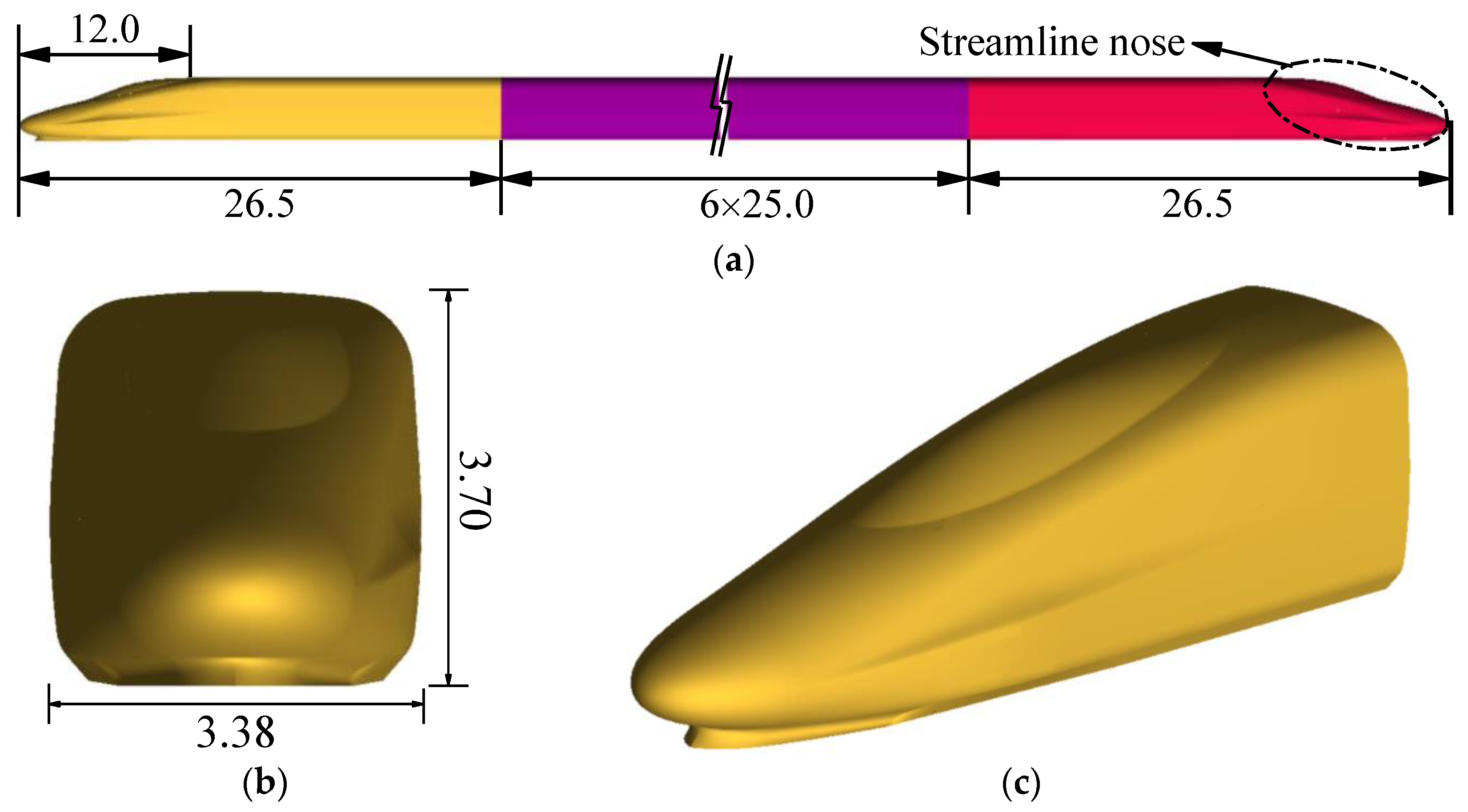
2.3. Tunnel and Train Models

A typical double-track HSR tunnel in China is adopted in our study. The configuration of the tunnel is shown in Figure 1. The center-to-center distance of two tracks is 5.0 m. The internal cross-sectional area and the length of the tunnel are 100 m2 and 1000 m, respectively. A CRH380A vehicle is modelled (Figure 2). As the accessory components of the HSR train (such as roof pantographs and handlebars) have negligible influences on the simulation results; they are not considered to improve computational efficiency. The constant cross-sectional area of the train body is 11.22 m2. The blockage ratio is 0.11. The train speed (v) in our simulation varies from 275 km/h to 400 km/h.

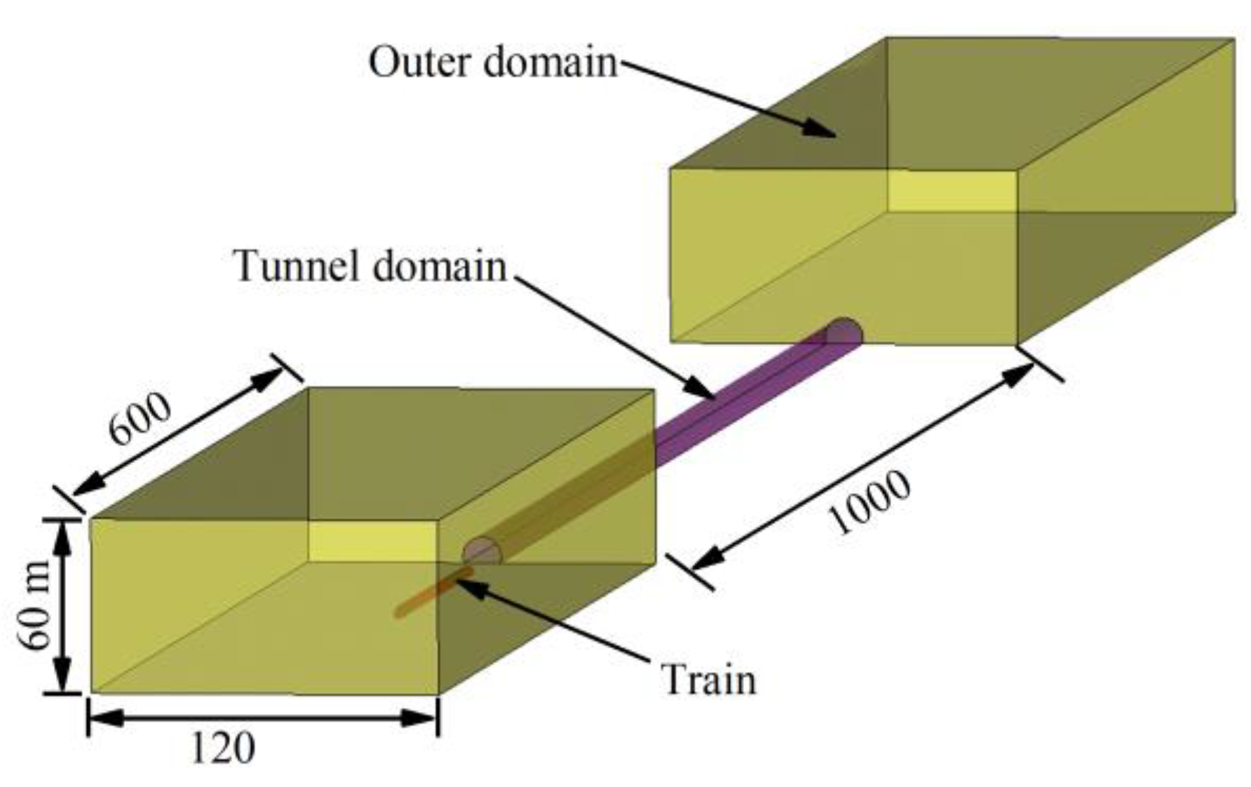
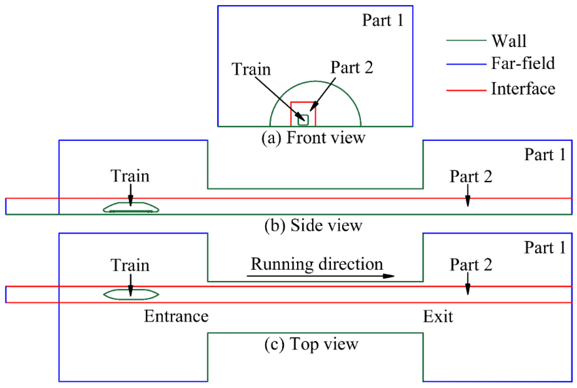
2.4. Computational Domain

The computational domain of our simulation includes a tunnel domain and two outer domains, as shown in Figure 3. The two outer domains are identical cuboids. The dimensions of these two outer domains are large enough to ensure that airflows inside the tunnel can be fully developed [30]. The starting location of the HSR train is placed 50 m in front of the tunnel entrance [31,32].

2.5. Boundary Conditions

The boundary conditions of our study are shown in Figure 4. The computational domain is divided into stationary part 1 and sliding part 2 to realize the relative movement between train and tunnel. The common surfaces of stationary part 1 and sliding part 2 are set as the interface. The top, two sides, front, and back surfaces of stationary part 1 are set as the pressure far-field. The bottom surface of stationary part 1 is set as the no-slip solid-wall [33]. The surfaces of stationary part 1, nearby the tunnel entrance and exit, are also set as the no-slip solid-wall. The top and two sides surfaces of sliding part 2 are set as the interface. The front and back surfaces are set as the pressure far-field, and the bottom surface is set as the no-slip solid-wall. The surfaces of tunnel wall and train body are set as the no-slip solid-wall. The pressure far-field allows pressure waves to penetrate without reflection. The interface allows the exchange of information between stationary part 1 and sliding part 2. The no-slip solid-wall allows pressure waves to reflect back from the wall.

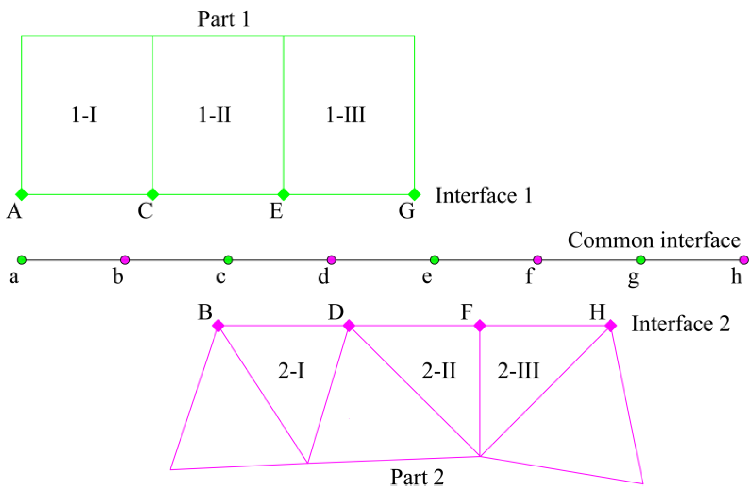
2.6. Sliding Mesh Method

The sliding mesh method has been widely adopted to simulate the running train in the tunnel [34]. Compared with the dynamic mesh method, the sliding mesh method updates the mesh without mesh-deformation and mesh-regeneration during the simulation. As a result, the calculation time required for the sliding mesh method is less. Thus, the sliding mesh method is applied in our simulation. The information exchange of airflows inside the computational domain can be accomplished by the interfaces. The schematic diagram of information exchange on the interface of the sliding mesh method is shown in Figure 5. When the sliding grid part 1 moves toward the right, the relative motion between grid part 1 and part 2 forms a common interface. The information on airflows is transmitted from zone 1-I, 1-II, and 1-III to zone 2-I, 2-II, and 2-III, respectively. The number of intersectional grids on the common interface changes when the interface 1 of part 1 moves relative to the interface 2 of part 2. The information of airflows passing through the common interface is calculated by the intersectional grids on the common interface. Thus, the information on airflows can be exchanged between adjacent parts.

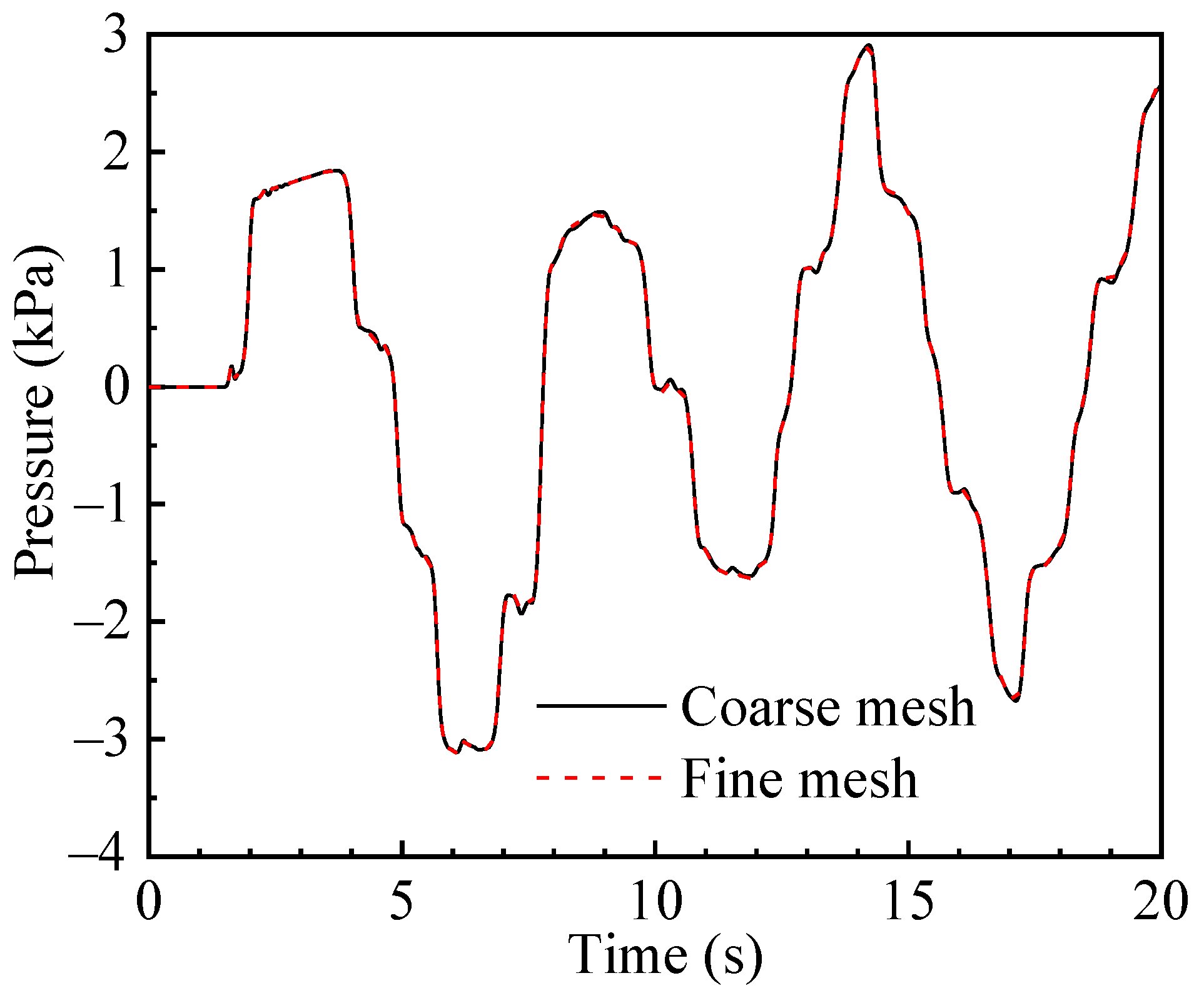
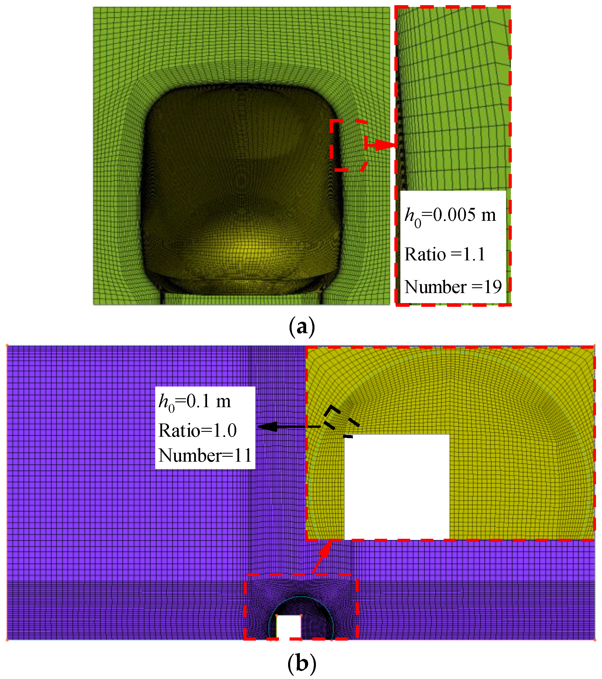
2.7. Grid Generation

The surface meshes of train nose and tunnel portal are shown in Figure 6. The hexahedral mesh is adopted in grid generation. The quality of the near-wall mesh can be evaluated by the dimensionless distance y+. The y+ values of train surface and tunnel wall in our simulation are controlled between 30 and 180 for the train speed varies from 275 km/h to 400 km/h, which meet the requirements of the standard [35]. The elements nearby the train streamline nose are refined manually as these regions have significant influences on the simulation results.
To study the influences of mesh density on the calculation results, two kinds of mesh densities, coarse mesh (16 million) and fine mesh (20 million), are used. In our simulation, the train speed and the tunnel length are 350 km/h and 1000 m, respectively. The comparations of aerodynamic pressure time histories calculated by coarse mesh and fine mesh are shown in Figure 7. The differences between the results obtained by the two mesh densities are negligible. The difference between the maximum positive peaks (maximum negative peaks) of these two mesh densities is only 1.0% (0.2%). Thus, the coarse mesh density is fair enough, and is used in the subsequent numerical simulations.

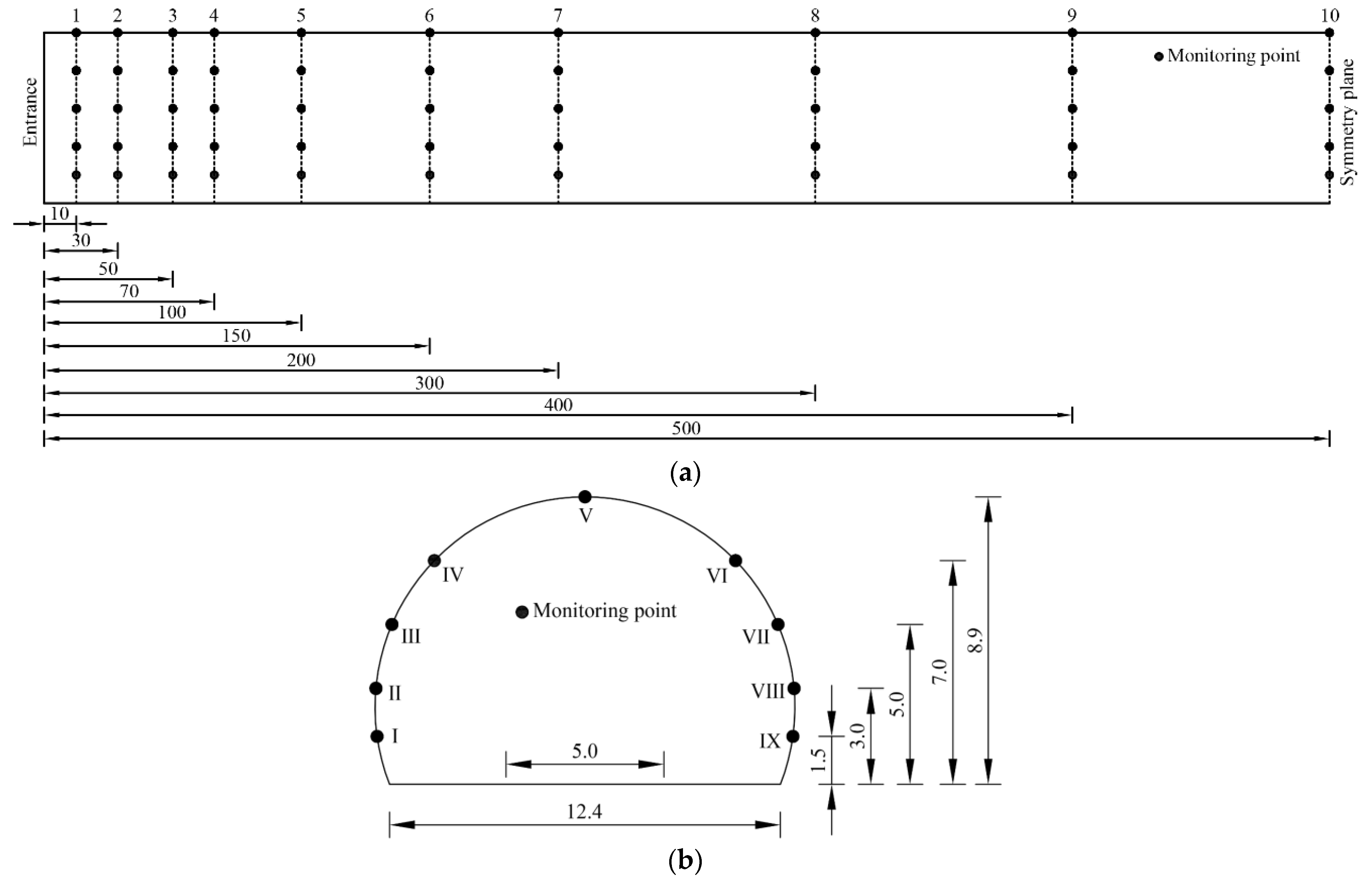
2.8. Layout of Monitoring Points
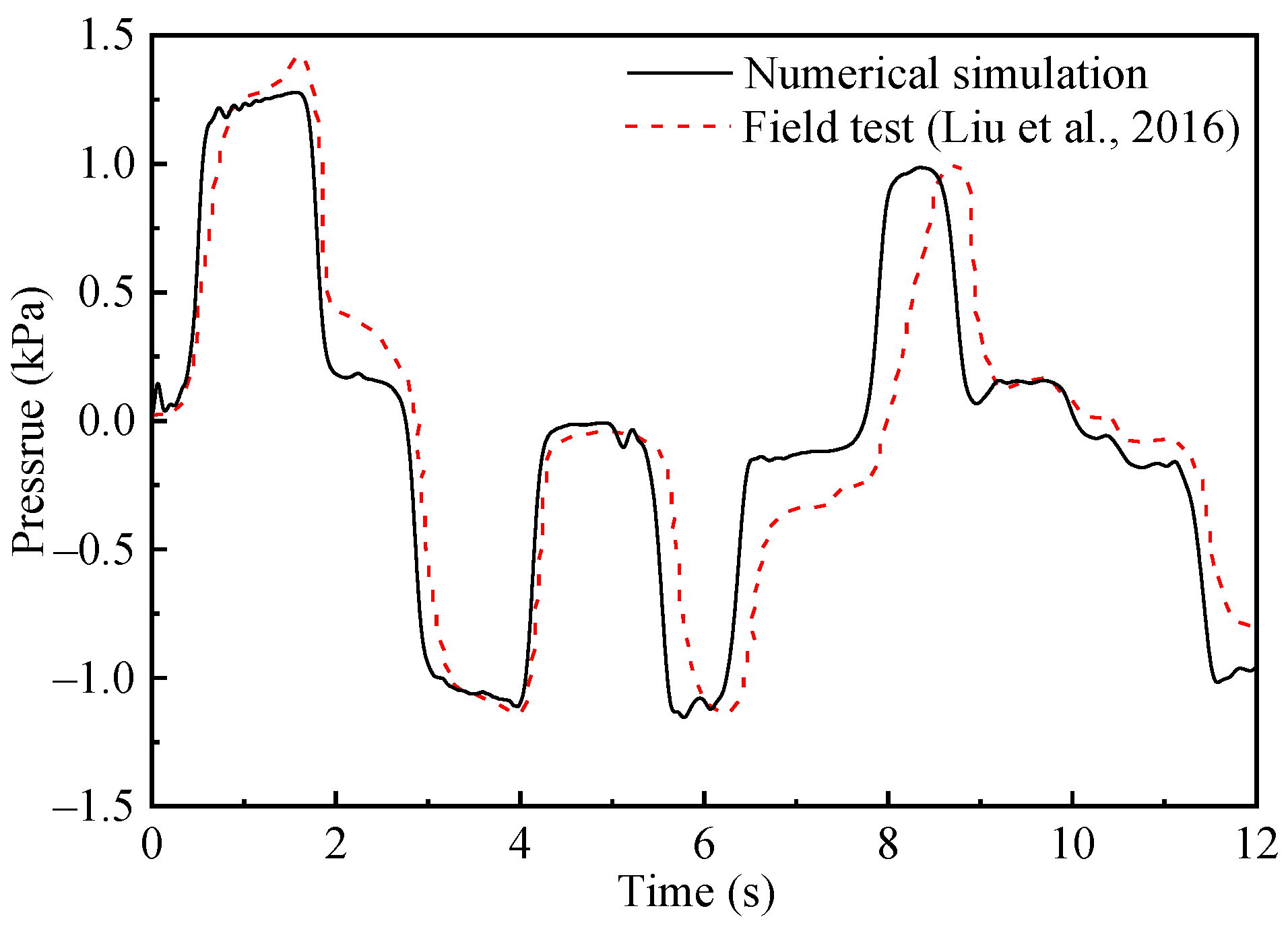
The layouts of monitoring points in the longitudinal section and cross section of the tunnel are shown in Figure 8. A total of 19 monitoring sections are arranged at different locations along the tunnel. There are nine monitoring points on each monitoring section.
We use the labels in the form of “1-II” to indicate the locations of monitoring points on the tunnel wall. The Arabic numerals in the labels show the cross-section ID, and the Roman numerals show the ID of the monitoring points in each monitoring section. For example, monitoring point 1-II indicates the second monitoring point on the first monitoring cross section.

3. Validation

To determine the values of input parameters in our simulation, the numerical results are compared with the field test results. A series of field tests were conducted on the Beijing-Shanghai high-speed railway line [36]. The length of CRH2C train and double-track tunnel were 200 m and 1005 m, respectively. The cross-sectional area of tunnel was 100 m2. The pressure sensors were installed on tunnel wall 1.5 m above the floor and 140 m from the entrance. The train speed of field tests was 300 km/h. The numerical simulation is performed in the same conditions as those of the field test. The aerodynamic pressures obtained by numerical simulation and field test are shown in Figure 9. The aerodynamic pressures obtained by the numerical simulation agree well with the field test results. The differences in the maximum positive peak, maximum negative peak, and maximum peak-peak values between these two methods are 9.8%, 2.1%, and 6.9%, respectively. As many factors, such as, temperature, humidity, and discontinuities, are not considered in the numerical simulation, there is a small difference between the time histories of aerodynamic pressures obtained by numerical simulation and field test. Generally, the numerical simulation can reasonably predict the field monitoring data. Therefore, the values of input parameters in the numerical simulation are suitable, and they can be used in the subsequent analysis.

4. Results

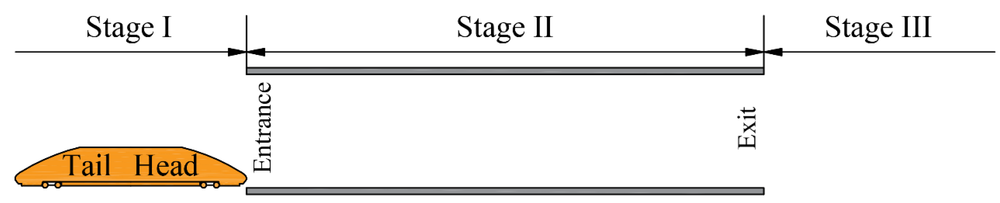
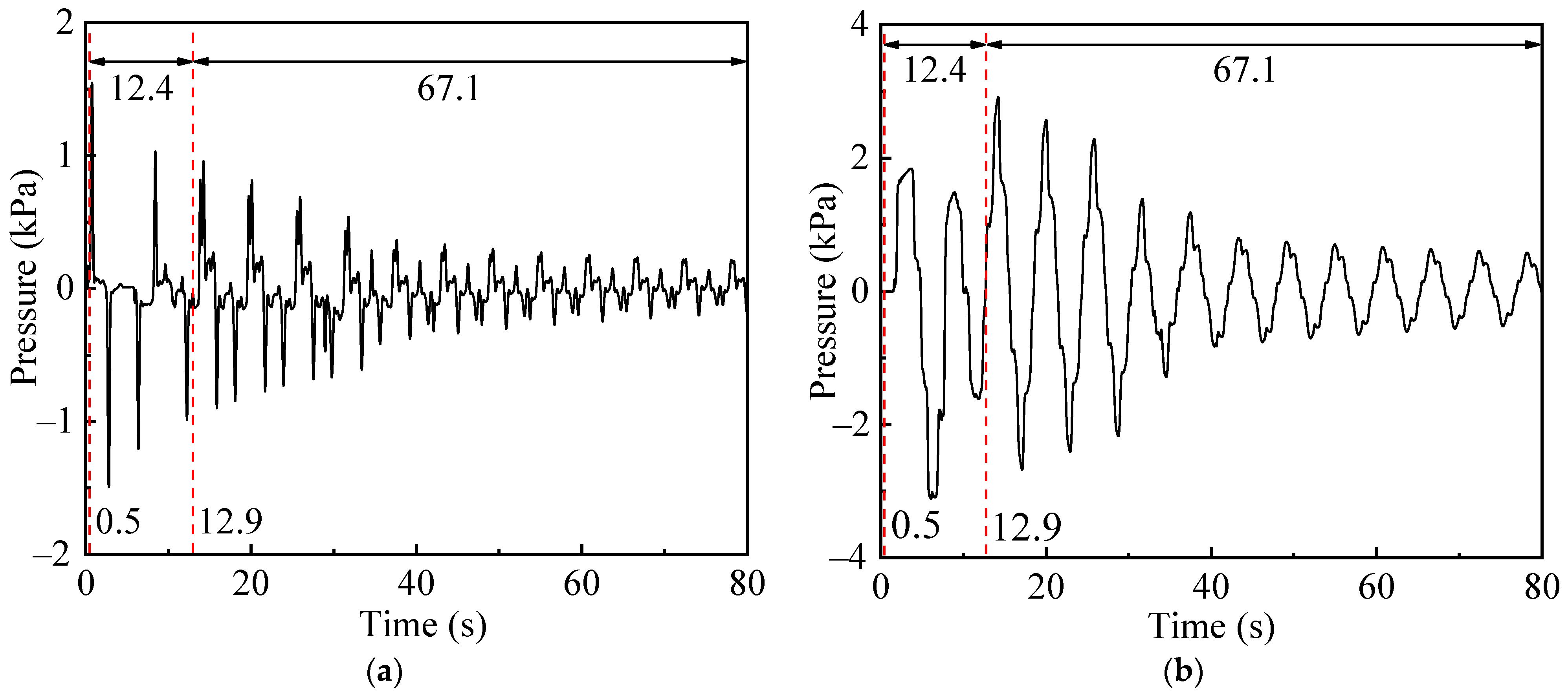
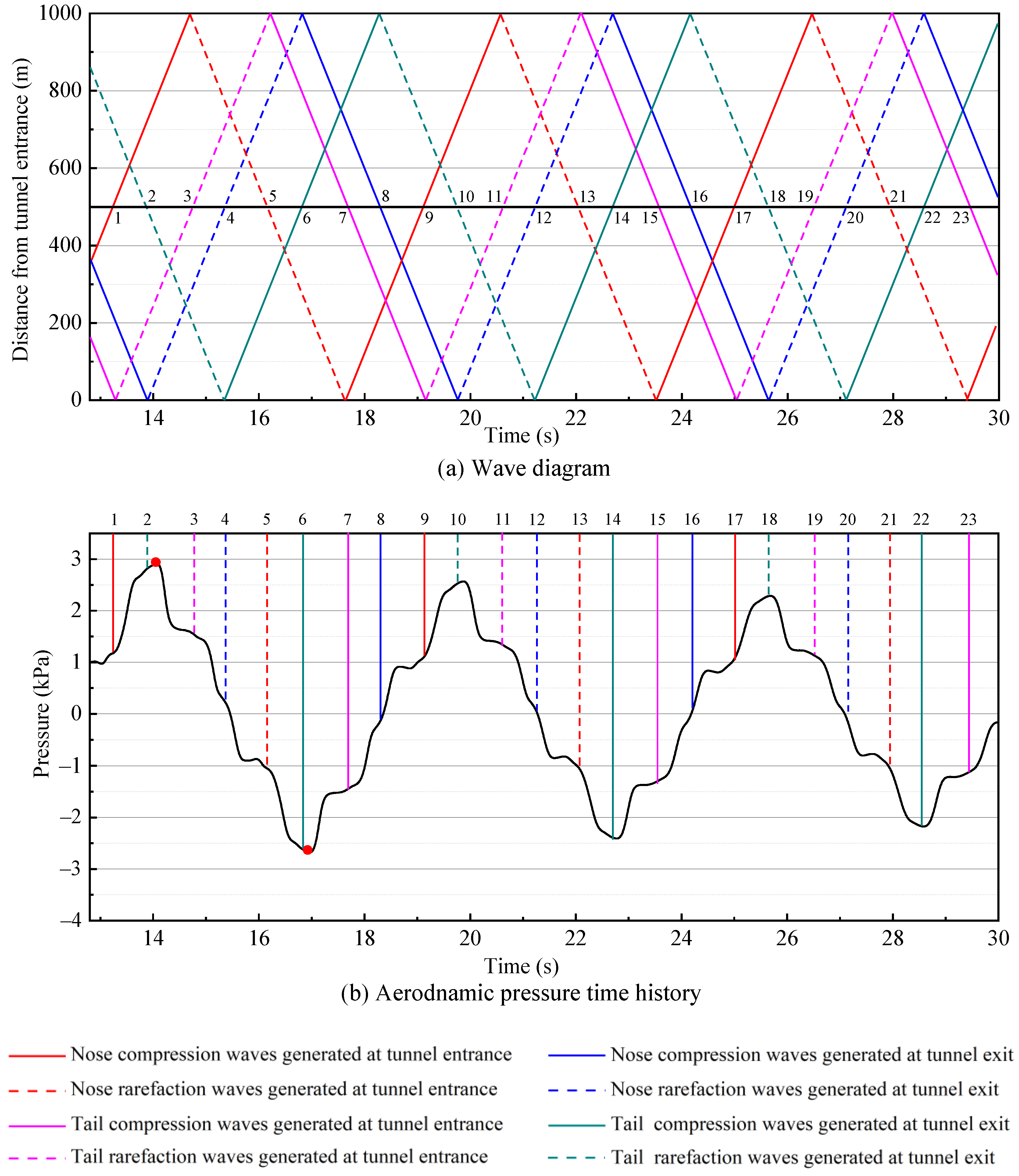
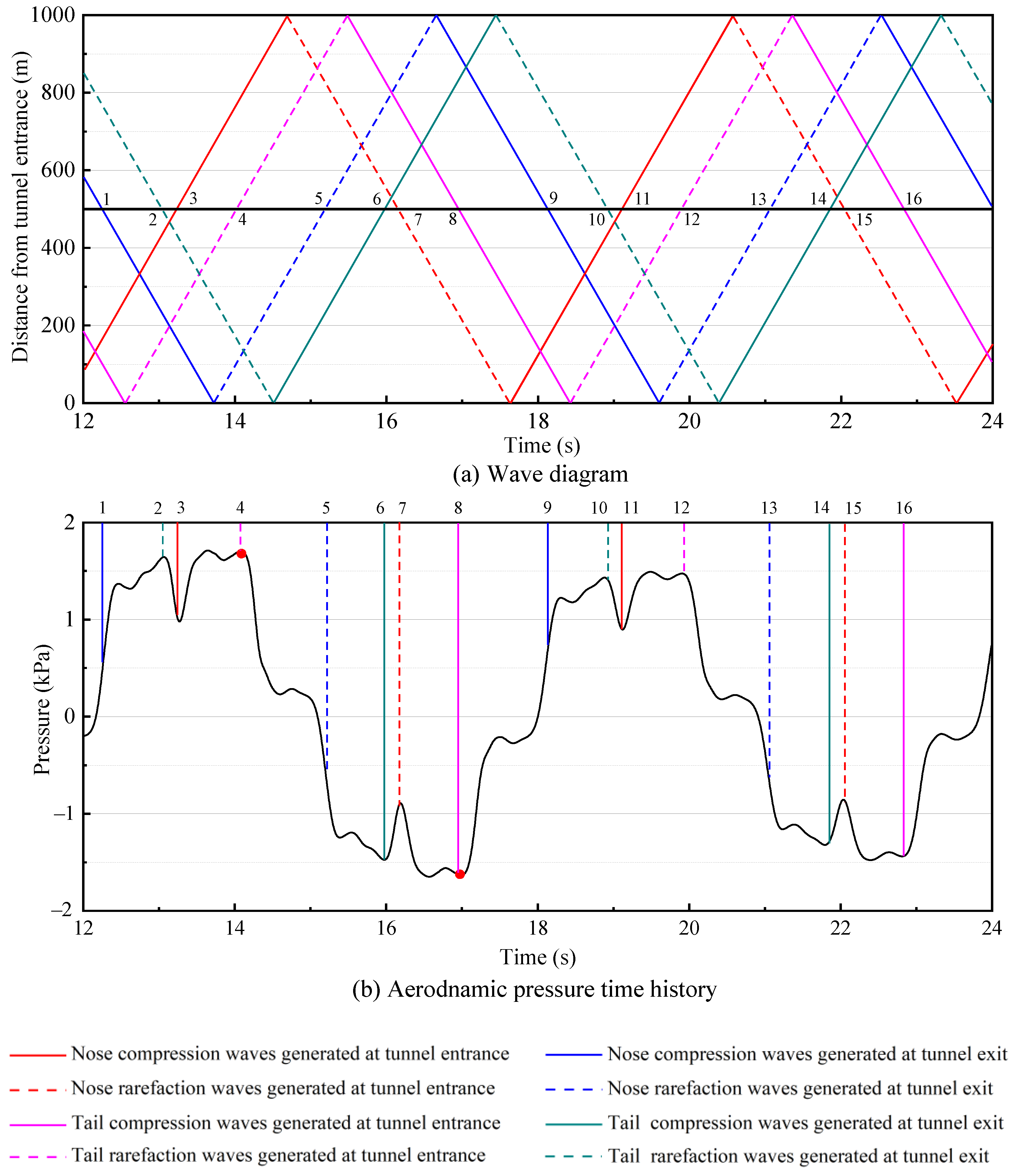
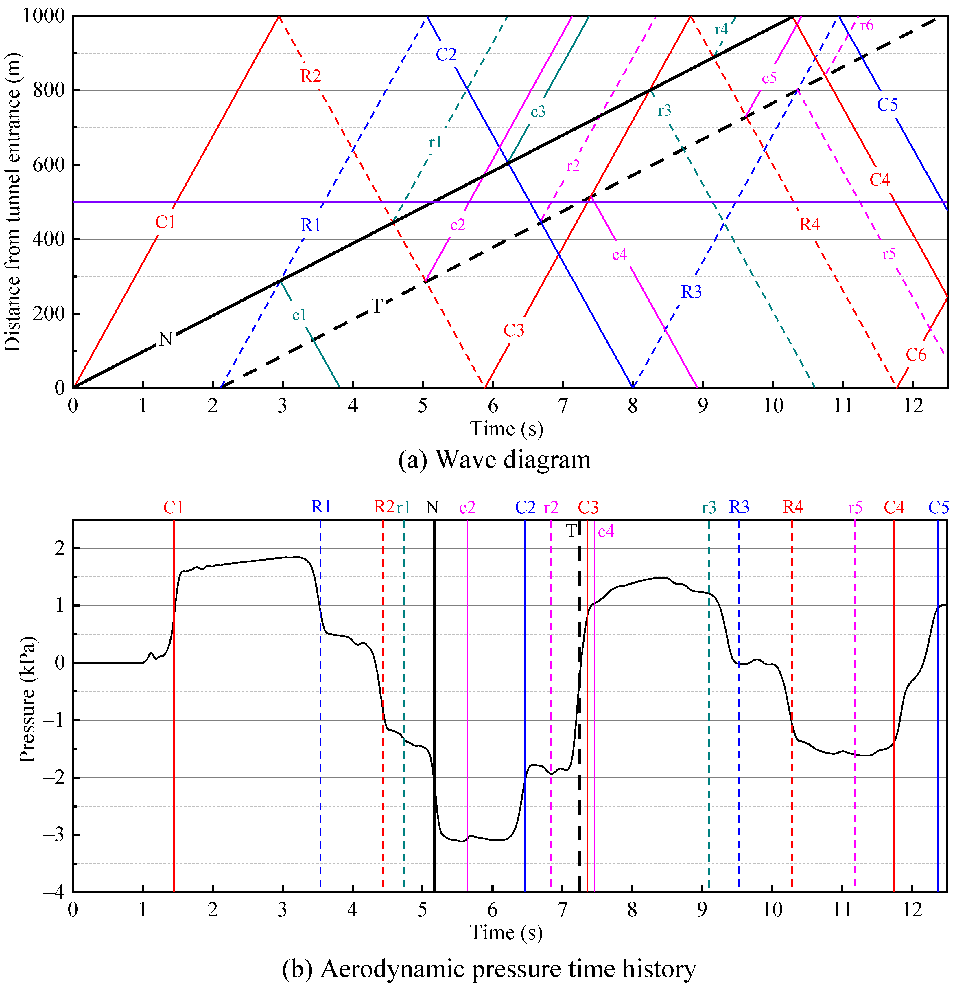
4.1. Typical Stages of Time History of Aerodynamic Pressures

To facilitate the illustration, the process of a single high-speed train travelling through a railway tunnel is divided into three stages (Figure 10). Stage I: before the train nose enters the entrance; Stage II: while the train body runs inside the tunnel; Stage III: after the train tail leaves the exit. Noted, the length of tunnel is longer than that of train [8].
In the case of a single high-speed train travels through a 1000 m long railway tunnel with a speed of 350 km/h (97.22 m/s), the development of aerodynamic pressures with time at some specific monitoring points are shown in Figure 11. It takes 0.5 s from starting for the HSR train nose to arrive at the tunnel entrance. It takes 12.9 s from starting for the train tail to leave the exit. After the train tail leaves the exit, the tunnel aerodynamic pressures last for 67.1 s until the peak pressure value reduces to about 10 % of the maximum peak pressure value of Stage III. It takes 0.15 s (50 m / 340 m/s = 0.15 s) for the initial pressure wave produced by the running of a train to reach the entrance in our designed scenario. Thus, the duration of aerodynamic pressures of Stage I is 0.35 s (0.5 s − 0.15 s = 0.35 s), and the duration of Stage II is 12.4 s (12.9 s − 0.5 s = 12.4 s). The duration of Stage II is about 35.4 times that of Stage I, and the duration of Stage III is about 197.1 times that of Stage I. The maximum positive peaks of monitoring point 2-V in Stages I, II, and III are 0.18 kPa, 1.54 kPa, and 0.95 kPa, respectively. The maximum positive peak in Stage II is about 8.6 times that in Stage I. The maximum positive peak in Stage III is about 5.3 times that in Stage I.
The peak pressures and the duration of Stage I are negligible in comparison to those of Stage II and Stage III. Therefore, the previous studies did not pay attention to the aerodynamic pressures of Stage I. However, considering the entire tunnel life cycle, the total duration of aerodynamic pressures and the total number of peak pressures of Stage I cannot be ignored. For example, a total of 195 pairs of high-speed trains travel on the Guangzhou-Shenzhen HSR line every day in China. The design life of an HSR tunnel is 100 years [8]. The total duration of aerodynamic pressures and the total amount of peak pressures of Stage I are 1384 h and 1.42 × 10⁷, respectively.
The maximum peak pressure of Stage I is much lower than the fracture strength of tunnel lining, and the total number of peak pressures is much higher than 106. Thus, the fatigue damage of the tunnel lining produced by the aerodynamic pressures of Stage I can be analyzed by the method of high-cycle fatigue [37]. To comprehensively investigate the long-term influences of aerodynamic effects on tunnel lining, the aerodynamic pressures of Stage I should be considered, especially near tunnel portals.

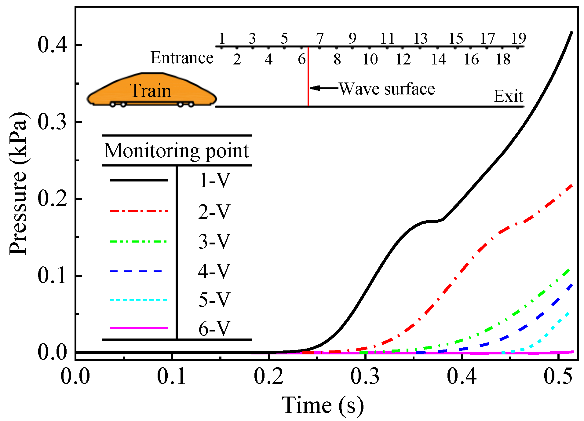
4.2. Aerodynamic Pressures in Stage I

When the train nose arrives at the entrance at a speed of 350 km/h, the aerodynamic pressure time histories at some specific monitoring points are shown in Figure 12. It takes 0.18 s (60 m / 340 m/s = 0.18 s) for the initial pressure wave produced by running of train to reach the monitoring point 1-V. When the train nose arrives at the entrance, the propagation distance of the initial pressure wave is 174.86 m (340 m/s × (50 m/97.22 m/s) = 174.86 m). The airflows from the tunnel entrance to the initial wave surface are disturbed by the initial pressure wave. As a result, the aerodynamic pressures are recorded from monitoring section 1 to monitoring section 6. Meanwhile, the airflows from the initial wave surface to the tunnel exit are undisturbed.
The distributions of the maximum peak pressures on the tunnel vault along the tunnel at different train speeds are shown in Figure 13. When the train nose arrives at the entrance, the propagation distances of the initial pressure waves at different train speeds are shown in Table 1. The peak pressure values of the monitoring points located at 200 m from tunnel entrance are not available when the train speed is faster than 300 km/h. The characteristics of maximum peak pressures on the tunnel vault along the tunnel’s longitudinal axis at different train speeds are similar. The maximum peak pressure decreases with increasing distance from the entrance. The maximum peak pressure increases with increasing train speed.
The maximum peak pressures at different train speeds of monitoring point 1-V and the related fitting curve are shown in Figure 14. The ‘x’ and ‘y’ show the train speed and the maximum peak pressure, respectively. The maximum peak pressure on tunnel vault increases linearly with increasing train speed, and the value of the adjusted coefficient of determination R2 is 0.99.

4.3. Aerodynamic Pressures in Stage II

Most previous studies in the field of the aerodynamic pressure waves inside tunnel focused on the behaviours in Stage II. The reflection of pressure waves from tunnel portals was widely investigated [38]. However, the reflection and transmission of pressure waves associated with the running train inside the tunnel have not been substantially explored, which have notable influences on the tunnel lining pressure. To cater to this issue, we systematically analyze the development of the pressure waves associated with the train body in this research.
The schematic diagram of propagation and reflection of a pressure wave between tunnel wall and train body is shown in Figure 15. When a compression wave Pa arrives at train tail, the effective sectional area of the airspace inside the tunnel is suddenly contracted due to the train. Then, most of the pressure wave Pa continues to transmit as a compression wave, and the magnitude of transmitted wave Pta is larger than Pa. The pressure wave Pa is partially reflected back as a compression wave, and the magnitude of the reflected wave Pra is smaller than Pa. When the compression wave Pta arrives at train nose, the effective sectional area of the airspace is suddenly enlarged, and the magnitude of transmitted wave Ptta is decreased. The reflected wave Prta turn into a rarefaction wave. Noted, the reflected wave is inverted (turning upside down) if the incident pressure wave disturbs a more massive medium, and the reflection is upright if the incident wave disturbs a less massive medium. The transmission of a pressure wave from the train nose to tail is similar to that from tail to nose. In fact, a pressure wave is partially reflected and partially transmitted at the boundary between media (i.e., tunnel portals, trains inside the tunnel). Therefore, numerous pressure waves are generated and propagate inside the tunnel, of which the superposition results in a complex pressure field on tunnel lining. Because of the friction effects of tunnel wall and train body, the intensity of pressure waves gradually decreases and ultimately disappears.
The relationship between the wave diagram and the pressure variations of monitoring point 10-V in Stage II is shown in Figure 16. The train speed is 350 km/h. In Figure 16a, the solid lines (with letters C and c) and dotted lines (with letters R and r) denote compression and rarefaction waves, respectively. The letters N and T denote the running paths of train nose and tail inside the tunnel, respectively. The paths C1 and R1 denote the initial pressure waves produced by the entering of train nose and tail, respectively. Except for C1 and R1, the uppercase letters (C and R) denote the reflected waves from tunnel portals. The lowercase letters (c and r) denote the reflected waves from the train nose and tail. The Arabic numerals denote the sequence of the reflected waves from a boundary (portal or train body) in the form of compression or rarefaction waves. As the intensity of the reflected wave from the train body is smaller than that of the incident wave, the subsequent reflections of this reflected wave are ignored. As a result, multiple pressure waves move between the tunnel portals during a train travelling in the tunnel. The recorded aerodynamic pressures of monitoring point 10-V, 500 m from both tunnel portals, are shown in Figure 16b. The vertical lines represent the moments at which the train nose, train tail, and pressure waves arriving at the monitoring section.
When the compression waves and the train tail arrive at the monitoring section, positive leaps of the monitoring pressure are produced. When the rarefaction waves and the train nose arrive at the monitoring section, negative drops are generated. The aerodynamic pressure time history of a point on tunnel lining is a superposition of numerous pressure waves [39]. The aerodynamic pressure field of the tunnel lining is complex, which varies with location and time in Stage II.
The distributions of three types of maximum peak pressures (positive peak, negative peak, and peak-to-peak pressures) along the tunnel vault in Stage II are shown in Figure 17. The three types of maximum peak pressure values of the points near tunnel middle section are generally larger than those of the points near tunnel portals. The relationships between the maximum peak pressure value of tunnel vault and the train speed of three typical tunnel cross section in Stage II are shown in Figure 18. The maximum peak pressure value increases with increasing train speed. There is an approximately linear relationship between each of the three types of maximum peak pressure value and the train speed raised to the power from 1.12 to 2.33 except for the boundary condition 0 kPa at 0 km/h.

4.4. Aerodynamic Pressures in Stage III

The wave diagram and the aerodynamic pressure time history of monitoring point 10-V in Stage III are shown in Figure 19. The train speed is 350 km/h. After train tail leaves the exit, the pressure field of tunnel lining is produced by the reflections of pressure waves from tunnel portals. The solid and dotted lines denote compression and rarefaction waves, respectively. The red and magenta lines denote pressure waves produced by the entering of train nose and tail, respectively. The blue and green lines denote pressure waves produced by the leaving of train nose and tail, respectively. As the energy of the pressure waves reflected from the train nose and tail is relatively small and has been reduced by the friction effect in Stage II, these reflected waves are ignored in Stage III.
The aerodynamic pressure time history presents a periodic variation due to the periodic reflections of the pressure waves from tunnel portals. The period of the aerodynamic pressures is mainly determined by tunnel length and wave speed. The pressure wave period can be defined as Tac = 2 L/c (L: tunnel length, c: sonic speed). The energy of pressure waves is gradually reduced by the dissipations at tunnel portals and the frictions on boundary surfaces (e.g., tunnel wall and track). Therefore, the amplitude of the aerodynamic pressures decreases with time. The amplitude of the aerodynamic pressures is increased after two or more pressure waves, with the disturbances along the same line, arriving at the monitoring section. Moreover, the amplitude of the aerodynamic pressures is decreased after two pressure waves, with the disturbances along the different lines, arriving at the monitoring section.
The distributions of the maximum peak pressures along the tunnel vault are shown in Figure 20. The maximum peak pressure values of the points near tunnel middle section are generally larger than those near tunnel portals.
The relationships between the maximum peak pressure and the train speed of specific monitoring points in Stage III are shown in Figure 21. The three types of maximum peak pressure values of the points near tunnel portals increase with increasing train speed. The three types of maximum peak pressure of tunnel middle section are more complex than those near tunnel portals. There are one or more turning points of these three types of maximum peak pressure of tunnel middle section.
As shown in Figure 19, when the train speed is 350 km/h, the aerodynamic pressure of the point near tunnel middle section achieves the maximum positive peak at 14.1 s. After three consecutive rarefaction waves pass through the monitoring section, the aerodynamic pressure achieves the maximum negative peak at 16.9 s. When the train speed is 375 km/h, the aerodynamic pressure of the point near tunnel middle section achieves the maximum positive peak at 14.2 s (Figure 22). After two rarefaction waves and one compression wave passe through the monitoring section, the aerodynamic pressure achieves the maximum negative peak at 17.0 s. As a result of the superimposed effect of pressure waves, the maximum negative peak pressure value of the point near tunnel middle section decreases after train speed increases from 350 km/h to 375 km/h. The existence of other turning points can also be explained by the superimposed effect of pressure waves.

5. Conclusions

To study the influences of high-speed train speed on tunnel aerodynamic pressures, we carry out a series of three-dimensional numerical simulations. The input parameters of our simulations are verified by field monitoring data. The process of a single high-speed train travelling through a railway tunnel is divided into three stages according to the spatial relationship between train and tunnel. The influences of high-speed train speed on tunnel aerodynamic pressures of these three stages are systematically studied. The main results are as follows:
(1) The peak pressure values at different train speeds are much lower than the fracture strength of tunnel lining, and the total number of peak pressures during the entire life cycle of tunnel in Stage I is much higher than 106. Thus, the aerodynamic fatigue damage of tunnel lining of Stage I can be calculated by the method of high-cycle fatigue.
(2) The characteristics of maximum peak pressure values acting on the tunnel vault along the tunnel’s longitudinal axis at different train speeds are similar in Stage I. The maximum peak pressure value decreases with increasing distance from the entrance and increases with increasing train speed.
(3) Three types of maximum peak pressure values (positive peak, negative peak, and peak-to-peak pressures) increase with increasing train speed in Stage II. There is an approximately linear relationship between each of these three types of maximum peak pressure values and high-speed train speed raised to the power from 1.12 to 2.33.
(4) The three types of maximum peak pressure values of the points near tunnel portals increase with increasing train speed in Stage III. These three types of maximum peak pressure of the tunnel middle section at different train speeds are more complex than those near the tunnel portals, and there is one or more turning point of the curves due to the superimposed effects of different pressure waves.

Author Contributions

J.D.: Conceptualization, formal analysis, software. Q.F.: Funding acquisition, Supervision, Validation. J.W.: Investigation, Writing-review & editing, Visualization. G.W.: Formal analysis, Data curation. All authors have read and agreed to the published version of the manuscript.

Funding

This research was funded by the Natural Science Foundation of Beijing, China grant number 8202037, and the Key Project of High-speed Rail Joint Fund of National Natural Science Foundation of China grant number U1934210.

Institutional Review Board Statement

Not applicable.

Informed Consent Statement

Not applicable.

Data Availability Statement

Data are contained within this article.

Acknowledgments

The authors thank the reviewers for their great help on the article during its review progress.

Conflicts of Interest

The authors declared that there is no conflict of interest.

References

  1. Baron, A.; Mossi, M.; Sibilla, S. The alleviation of the aerodynamic drag and wave effects of high-speed trains in very long tunnels. J. Wind. Eng. Ind. Aerodyn. 2001, 89, 365–401. [Google Scholar] [CrossRef]
  2. Schmitt, F.G. About Boussinesq’s turbulent viscosity hypothesis: Historical remarks and a direct evaluation of its validity. Comptes Rendus Mécanique 2007, 335, 617–627. [Google Scholar] [CrossRef] [Green Version]
  3. Doi, T.; Ogawa, T.; Masubuchi, T.; Kaku, J. Development of an experimental facility for measuring pressure waves generated by high-speed trains. J. Wind. Eng. Ind. Aerodyn. 2010, 98, 55–61. [Google Scholar] [CrossRef]
  4. Niu, J.; Zhou, D.; Liang, X.; Liu, T.; Liu, S. Numerical study on the aerodynamic pressure of a metro train running between two adjacent platforms. Tunn. Undergr. Space Technol. 2017, 65, 187–199. [Google Scholar] [CrossRef]
  5. Rivero, J.M.; González-Martínez, E.; Rodríguez-Fernández, M. A methodology for the prediction of the sonic boom in tunnels of high-speed trains. J. Sound Vib. 2019, 446, 37–56. [Google Scholar] [CrossRef]
  6. Li, W.; Liu, T.; Chen, Z.; Guo, Z.; Huo, X. Comparative study on the unsteady slipstream induced by a single train and two trains passing each other in a tunnel. J. Wind. Eng. Ind. Aerodyn. 2020, 198, 104095. [Google Scholar] [CrossRef]
  7. Li, X.-H.; Deng, J.; Chen, D.-W.; Xie, F.-F.; Zheng, Y. Unsteady simulation for a high-speed train entering a tunnel. J. Zhejiang Univ. A 2011, 12, 957–963. [Google Scholar] [CrossRef]
  8. Du, J.; Fang, Q.; Wang, G.; Zhang, D.; Chen, T. Fatigue damage and residual life of secondary lining of high-speed railway tunnel under aerodynamic pressure wave. Tunn. Undergr. Space Technol. 2021, 111, 103851. [Google Scholar] [CrossRef]
  9. Ko, Y.-Y.; Chen, C.-H.; Hoe, I.-T.; Wang, S.-T. Field measurements of aerodynamic pressures in tunnels induced by high speed trains. J. Wind Eng. Ind. Aerodyn. 2012, 100, 19–29. [Google Scholar] [CrossRef]
  10. Liu, T.-H.; Jiang, Z.-H.; Li, W.-H.; Guo, Z.-J.; Chen, X.-D.; Chen, Z.-W.; Krajnovic, S. Differences in aerodynamic effects when trains with different marshalling forms and lengths enter a tunnel. Tunn. Undergr. Space Technol. 2018, 84, 70–81. [Google Scholar] [CrossRef]
  11. Liu, T.-H.; Tian, H.-Q.; Liang, X.-F. Design and optimization of tunnel hoods. Tunn. Undergr. Space Technol. 2010, 25, 212–219. [Google Scholar] [CrossRef]
  12. Zhang, L.; Yang, M.-Z.; Niu, J.-Q.; Liang, X.-F.; Zhang, J. Moving model tests on transient pressure and micro-pressure wave distribution induced by train passing through tunnel. J. Wind Eng. Ind. Aerodyn. 2019, 191, 1–21. [Google Scholar] [CrossRef]
  13. Howe, M.S. Mach number dependence of the compression wave generated by a high-speed train entering a tunnel. J. Sound Vib. 1998, 212, 23–36. [Google Scholar] [CrossRef]
  14. Murray, P.; Howe, M. Influence of hood geometry on the compression wave generated by a high-speed train. J. Sound Vib. 2010, 329, 2915–2927. [Google Scholar] [CrossRef]
  15. Munoz-Paniagua, J.; Garcia, J.G.; Crespo, A. Genetically aerodynamic optimization of the nose shape of a high-speed train entering a tunnel. J. Wind Eng. Ind. Aerodyn. 2014, 130, 48–61. [Google Scholar] [CrossRef] [Green Version]
  16. Chen, X.-D.; Liu, T.-H.; Zhou, X.-S.; Li, W.-H.; Xie, T.-Z.; Chen, Z.-W. Analysis of the aerodynamic effects of different nose lengths on two trains intersecting in a tunnel at 350 km/h. Tunn. Undergr. Space Technol. 2017, 66, 77–90. [Google Scholar] [CrossRef]
  17. Chu, C.-R.; Chien, S.-Y.; Wang, C.-Y.; Wu, T.-R. Numerical simulation of two trains intersecting in a tunnel. Tunn. Undergr. Space Technol. 2014, 42, 161–174. [Google Scholar] [CrossRef]
  18. Mei, Y.G.; Wang, R.L.; Xu, J.L.; Jia, Y.X.; Zhou, C.H. Numerical simulation of initial compression wave induced by a high-speed train moving into a tunnel. Chin. J. Comput. Mech. 2016, 33, 95–101. [Google Scholar] [CrossRef]
  19. Liu, F.; Yao, S.; Zhang, J.; Wang, Y.-Q. Field measurements of aerodynamic pressures in high-speed railway tunnels. Tunn. Undergr. Space Technol. 2018, 72, 97–106. [Google Scholar] [CrossRef]
  20. Rabani, M.; Faghih, A.K. Numerical analysis of airflow around a passenger train entering the tunnel. Tunn. Undergr. Space Technol. 2015, 45, 203–213. [Google Scholar] [CrossRef]
  21. Fang, Q.; Zhang, D.; Li, Q.; Wong, L.N.Y. Effects of twin tunnels construction beneath existing shield-driven twin tunnels. Tunn. Undergr. Space Technol. 2015, 45, 128–137. [Google Scholar] [CrossRef]
  22. Yang, W.; Deng, E.; Lei, M.; Zhang, P.; Yin, R. Flow structure and aerodynamic behavior evolution during train entering tunnel with entrance in crosswind. J. Wind Eng. Ind. Aerodyn. 2018, 175, 229–243. [Google Scholar] [CrossRef]
  23. Li, W.; Liu, T.; Huo, X.; Chen, Z.; Guo, Z.; Li, L. Influence of the enlarged portal length on pressure waves in railway tunnels with cross-section expansion. J. Wind Eng. Ind. Aerodyn. 2019, 190, 10–22. [Google Scholar] [CrossRef]
  24. Li, P.; Wei, Y.; Zhang, M.; Huang, Q.; Wang, F. Influence of non-associated flow rule on passive face instability for shallow shield tunnels. Tunn. Undergr. Space Technol. 2021, 119, 104202. [Google Scholar] [CrossRef]
  25. Fang, Q.; Wang, G.; Yu, F.; Du, J. Analytical algorithm for longitudinal deformation profile of a deep tunnel. J. Rock Mech. Geotech. Eng. 2021, 13, 845–854. [Google Scholar] [CrossRef]
  26. Huang, Y.-D.; Gao, W.; Kim, C.-N. A Numerical Study of the Train-Induced Unsteady Airflow in a Subway Tunnel with Natural Ventilation Ducts Using the Dynamic Layering Method. J. Hydrodyn. 2010, 22, 164–172. [Google Scholar] [CrossRef]
  27. Li, W.H.; Liu, T.H.; Zhang, J.; Chen, Z.W.; Chen, X.D.; Xie, T.Z. Aerodynamic study of two opposing moving trains in a tunnel based on different nose contours. J. Appl. Fluid Mech. 2017, 1, 54–65. [Google Scholar] [CrossRef]
  28. Liu, T.; Jiang, Z.; Chen, X.; Zhang, J.; Liang, X. Wave effects in a realistic tunnel induced by the passage of high-speed trains. Tunn. Undergr. Space Technol. 2019, 86, 224–235. [Google Scholar] [CrossRef]
  29. Liu, T.; Geng, S.; Chen, X.; Krajnovic, S. Numerical analysis on the dynamic airtightness of a railway vehicle passing through tunnels. Tunn. Undergr. Space Technol. 2020, 97. [Google Scholar] [CrossRef]
  30. Niu, J.; Sui, Y.; Yu, Q.; Cao, X.; Yuan, Y. Numerical study on the impact of Mach number on the coupling effect of aerodynamic heating and aerodynamic pressure caused by a tube train. J. Wind. Eng. Ind. Aerodyn. 2019, 190, 100–111. [Google Scholar] [CrossRef]
  31. Liu, T.-H.; Chen, Z.-W.; Chen, X.-D.; Xie, T.-Z.; Zhang, J. Transient loads and their influence on the dynamic responses of trains in a tunnel. Tunn. Undergr. Space Technol. 2017, 66, 121–133. [Google Scholar] [CrossRef]
  32. Jiang, Z.; Liu, T.; Chen, X.; Li, W.; Guo, Z.; Niu, J. Numerical prediction of the slipstream caused by the trains with different marshalling forms entering a tunnel. J. Wind. Eng. Ind. Aerodyn. 2019, 189, 276–288. [Google Scholar] [CrossRef]
  33. Launder, B.; Spalding, D. The numerical computation of turbulent flows. Comput. Methods Appl. Mech. Eng. 1974, 3, 269–289. [Google Scholar] [CrossRef]
  34. Niu, J.; Zhou, D.; Liu, F.; Yuan, Y. Effect of train length on fluctuating aerodynamic pressure wave in tunnels and method for determining the amplitude of pressure wave on trains. Tunn. Undergr. Space Technol. 2018, 80, 277–289. [Google Scholar] [CrossRef]
  35. National Railway Administration of the People’s Republic of China. Railway Applications—Aerodynamics—Part 4: Requirements for Train Aerodynamic Simulation; TB/T3503.4; China Railway Publishing House Co., Ltd.: Beijing, China, 2018.
  36. Liu, F.; Yao, S.; Liu, T.H.; Zhang, J. Analysis on aerodynamic pressure of tunnel wall of high-speed railways by full-scale train test. J. Zhejiang Univ. (Eng. Sci.) 2016, 43, 1383–1388. [Google Scholar] [CrossRef]
  37. Schijve, J. Fatigue of structures and materials in the 20th century and the state of the art. Int. J. Fatigue 2003, 25, 679–702. [Google Scholar] [CrossRef]
  38. Zhang, L.; Thurow, K.; Stoll, N.; Liu, H. Influence of the geometry of equal-transect oblique tunnel portal on compression wave and micro-pressure wave generated by high-speed trains entering tunnels. J. Wind. Eng. Ind. Aerodyn. 2018, 178, 1–17. [Google Scholar] [CrossRef]
  39. Shuanbao, Y.; Dilong, G.; Zhenxu, S.; Guowei, Y.; Dawei, C. Optimization design for aerodynamic elements of high speed trains. Comput. Fluids 2014, 95, 56–73. [Google Scholar] [CrossRef] [Green Version]
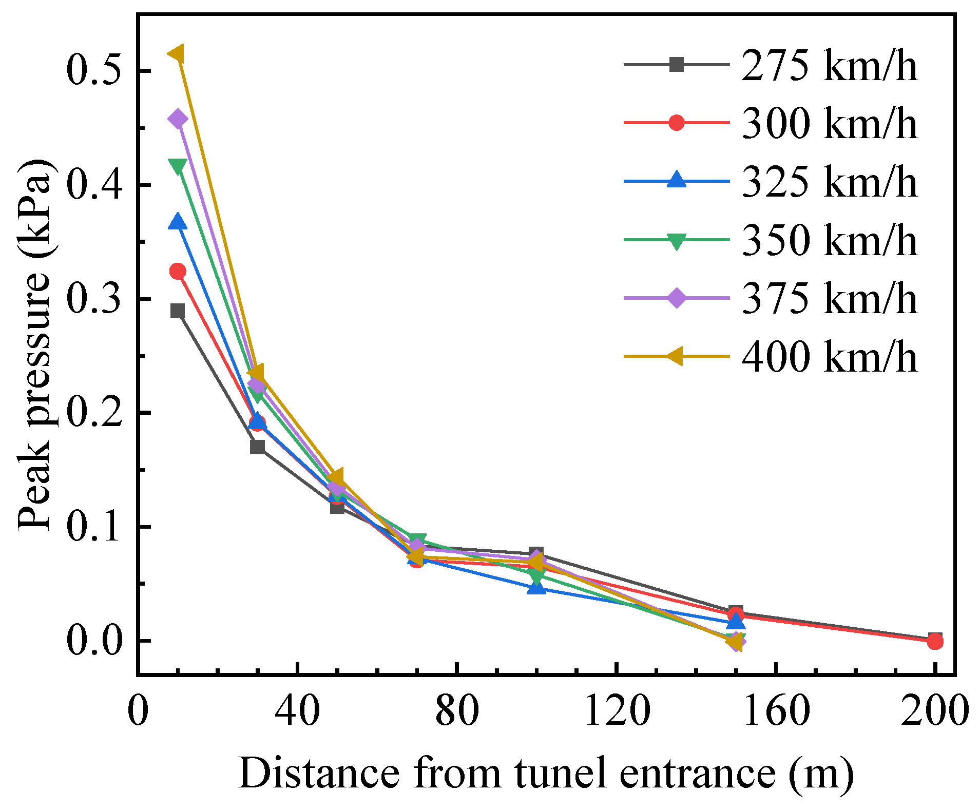
Figure 1. Configuration of tunnel (unit: m).
Applsci 12 00303 g001
Figure 2. Train model (unit: m). (a) Side view; (b) Front view; (c) Streamline nose.
Applsci 12 00303 g002
Figure 3. Computational domain (unit: m).
Applsci 12 00303 g003
Figure 4. Boundary conditions.
Applsci 12 00303 g004
Figure 5. Schematic diagram of information exchange on common interface of sliding mesh method.
Applsci 12 00303 g005
Figure 6. Surface meshes around train nose and tunnel portal. (a) Surface mesh of train nose; (b) Surface mesh of tunnel portal.
Applsci 12 00303 g006
Figure 7. Aerodynamic pressure time histories obtained by coarse mesh and fine mesh.
Applsci 12 00303 g007
Figure 8. Layouts of monitoring points (unit: m). (a) Longitudinal section; (b) Cross section.
Applsci 12 00303 g008
Figure 9. Aerodynamic pressures obtained by numerical simulation and field test.
Applsci 12 00303 g009
Figure 10. Spatial relationship between train and tunnel.
Applsci 12 00303 g010
Figure 11. Aerodynamic pressures time histories for typical monitoring points (v = 350 km/h). (a) Monitoring point 2-V; (b) Monitoring point 10-V; (c) Monitoring point 17-V.
Applsci 12 00303 g011aApplsci 12 00303 g011b
Figure 12. Time histories of aerodynamic pressure of typical monitoring points in Stage I (v = 350 km/h).
Applsci 12 00303 g012
Figure 13. Peak pressure acting on tunnel vault along tunnel’s longitudinal axis in Stage I.
Applsci 12 00303 g013
Figure 14. Peak pressure versus train speed of monitoring point 1-V in Stage I.
Applsci 12 00303 g014
Figure 15. Schematic of propagation and reflection of a pressure wave between tunnel wall and train body surface in Stage II. (Note: Pa: pressure wave, Pra: reflected wave of Pa, Pta: transmitted wave of Pa, Prta: reflected wave of Pta, Ptta: transmitted wave of Pta).
Applsci 12 00303 g015
Figure 16. Relationship between wave diagram and aerodynamic pressure of monitoring point 10-V in Stage II.
Applsci 12 00303 g016aApplsci 12 00303 g016b
Figure 17. Distributions of maximum peak pressures along tunnel vault in Stage II.
Applsci 12 00303 g017
Figure 18. Maximum peak pressures versus train speed of typical monitoring points in Stage II. (a) Maximum positive peak; (b) Maximum negative peak; (c) Maximum peak-to-peak value.
Applsci 12 00303 g018
Figure 19. Wave diagram and aerodynamic pressure time history of monitoring point 10-V in Stage III at train speed of 350 km/h.
Applsci 12 00303 g019
Figure 20. Distributions of maximum peak pressures along tunnel vault in Stage III.
Applsci 12 00303 g020
Figure 21. Maximum peak pressure values at different train speeds of typical monitoring points in Stage III. (a) Maximum positive peak; (b) Maximum negative peak; (c) Maximum peak-to-peak value.
Applsci 12 00303 g021
Figure 22. Wave diagram and aerodynamic pressure time history of monitoring point 10-V in Stage III at train speed of 375 km/h.
Applsci 12 00303 g022
Table 1. Propagation distances of initial pressure waves at different train speeds in Stage I.
Train speed (km/h)275300325350375400
Propagation distance (m)222.55204.00188.31174.86163.20153.00
Publisher’s Note: MDPI stays neutral with regard to jurisdictional claims in published maps and institutional affiliations.

