Best-Estimate for System Codes (BeSYC): A New Software to Perform Best-Estimate Plus Uncertainty Analyses with Thermal-Hydraulic and Safety System Codes for Both Fusion and Fission Scenarios

Abstract

The development and the validation of old and new software in relevant DEMO reactor conditions have been exploited in the latest years within the EUROfusion Consortium. The aim was to use—if possible—the software already validated for fission reactors and to fill the gaps with new ad-hoc software. As contribution to this effort, the Karlsruhe Institute of Technology (KIT) developed and tested a novel software to apply the Best-Estimate Model Calibration and Prediction through Experimental Data Assimilation methodology to the system codes RELAP5-3D, MELCOR 1.8.6, and MELCOR 2.2. This software is called Best-estimate for SYstem Codes (BeSYC), and it is developed as a MATLAB App. The application is in charge of applying the mathematical framework of the methodology, writing and executing the code runs required by the methodology, and printing the obtained results. The main goal of BeSYC is to wrap up the methodology in a software suitable to be used by any user through a simple graphical user interface. Albeit developed in the fusion research context, BeSYC can be applied to any reactor/scenario type supported by the specific system code. The goals of BeSYC, the mathematical framework, the main characteristics, and the performed verification and validation activities are described in this paper.

1. Introduction

The Best-Estimate Plus Uncertainty (BEPU) analysis has become one of the most important research topics in the nuclear field in the last 30 years [1]. To date, several BEPU methodologies have been developed [2], mainly in the frame of fission reactors, but they are becoming increasingly popular also for fusion reactors [3]. One of them is the Best-Estimate Model Calibration and Prediction through Experimental Data Assimilation methodology [4,5].

At the same time, huge efforts have been also spent on the validation of system codes in the frame of the EU-DEMO R&D [6,7]. Considering that most of the codes currently in use (RELAP5-3D, MELCOR 1.8.6 for fusion, SIMMER III, etc.) were and are developed in the frame of fission reactors, validation studies are required to ensure the applicability of such codes to the analysis of incidental transients in the typical conditions of fusion reactors.

The Karlsruhe Institute of Technology (KIT) is actively involved in both software development and validation. Recently, some of the efforts have been devoted to the development of a software to apply the Best-Estimate Model Calibration and Prediction through Experimental Data Assimilation methodology [4,5] to the RELAP5-3D and MELCOR 1.8.6 codes for code’s validation purposes (to ease the reading of the paper, hereinafter, the methodology is called “BEPU methodology”). This software is called Best-estimate for SYstem Codes (BeSYC; version 1; KIT: Karlsruhe, Germany), and it was developed as a MATLAB App. The aim of BeSYC is not only limited to the application of the BEPU methodology, but it also covers the writing and the execution of the code runs required to apply the BEPU methodology itself. The present paper describes the structure, the mathematical framework, and the validation of this software. This paper is published in conjunction with two other papers showing the application of BeSYC with both RELAP5-3D and MELCOR 1.8.6 codes against the data gathered from an experimental campaign on a helium-cooled first wall mock-up (FWMU) under Loss Of Flow Accident (LOFA) conditions [8,9]. Even if not yet used for any real-case scenario, the BeSYC software supports also MELCOR 2.2.

Brief History of the BeSYC Software

The idea to develop the BeSYC software started from a simple attempt to create a MATLAB script to apply the numerical framework related to the BEPU methodology in the post-test numerical analysis of an experimental campaign carried out at KIT [8]. However, since the early stage of development, it was noted that most of the efforts to apply the BEPU methodology would have been needed while writing the input decks required for the several code runs (the so-called sensitivity input decks). The execution of such code runs was also found to be a task requiring a relevant effort because the manual starting of more than 100 runs would have meant the presence of dead times between a run and the following. Not only this, but these tasks are also prone to human errors, especially considering the typical iterative process of “tuning and error fixing” of the input decks based on the achieved results.

For these reasons, the development of this simple script turned into the development of a much more complex tool capable of managing all these complex aspects. The development of the BeSYC software was grounded on three fundamental pillars: independency, modularity, and multi-platform availability:

• Independency because the tool is developed independently from any system code;
• Modularity since it is developed following a modular approach capable to ease the maintenance of the code itself and the introduction of new features;
• Multi-platform availability in view of the fact that the tool should run on each operative system for which the system code executables are available (Microsoft Windows© 7, 10, and 11 and Linux).

A further impulse to the development of BeSYC came when the number of options to run the BEPU methodology started to increase, i.e., when also the $C_{\alpha \alpha }$ and $C_{\alpha r}$ variance-covariance matrices started to be given as input data (see Section 2). This necessity pushed for the development of a Graphical User Interface (GUI) capable to guide the user into the creation of the BeSYC input files. In the same frame of time, the BeSYC software was also improved with the possibility to write and run a best-estimate input deck (for the system code in use) after the application of the BEPU methodology.

2. Theoretical Background of the Best-Estimate Methodology

The Best-Estimate Model Calibration and Prediction through Experimental Data Assimilation methodology is described in [4,5], and it is introduced in the BeSYC software. The two aforementioned papers provide an exhaustive description of the numerical framework, which is here only briefly recalled.

The BEPU methodology is a numerical framework based on the Bayes’ theorem and the information theory to assimilate experimental and computational information together with their uncertainties. A physical system is modelled in terms of equations relating the system state (dependent variables) with the system independent variables. Most of the terms in these equations are hard-coded in the code’s source code, but some of them are provided in the input deck (loss coefficients, wall thicknesses. etc.). These terms are called parameters ($\alpha$), and they are required by these equations to calculate the system responses ($r$), like pressures, temperatures, etc. The aim of the methodology is to provide best-estimated/calibrated values of these parameters and responses as well as a best-estimated/calibrated evaluation of their uncertainties.

Assuming a generic physical characterized by two parameters (${\alpha }_1$ and ${\alpha }_2$) and two experimental responses ($r_1$ and $r_2$) measured at n time nodes, the nominal values of both the parameters and the responses are represented as column vectors:

$$\alpha =\left(\begin{array}{c}{\alpha }_1^{t_1}\\ {\alpha }_2^{t_1}\\ ⋮\\ {\alpha }_1^{t_n}\\ {\alpha }_2^{t_n}\end{array}\right) r=\left(\begin{array}{c}{r}_1^{t_1}\\ r_2^{t_1}\\ ⋮\\ r_1^{t_n}\\ r_2^{t_n}\end{array}\right)$$

(1)

Both the parameters and the responses are affected by uncertainties that are expressed by means of two variance-covariance matrices ($C_{\alpha \alpha }$ and $C_{rr}$), arranged as:

$$C_{\alpha \alpha }=\left(\begin{array}{ccccc}{\sigma }_{{\alpha }_1}^{t_1}·{\sigma }_{{\alpha }_1}^{t_1}& {\sigma }_{{\alpha }_2}^{t_1}·{\sigma }_{{\alpha }_1}^{t_1}& & {\sigma }_{{\alpha }_1}^{t_n}·{\sigma }_{{\alpha }_1}^{t_1}& {\sigma }_{{\alpha }_2}^{t_n}·{\sigma }_{{\alpha }_1}^{t_1}\\ {\sigma }_{{\alpha }_1}^{t_1}·{\sigma }_{{\alpha }_2}^{t_1}& {\sigma }_{{\alpha }_2}^{t_1}·{\sigma }_{{\alpha }_2}^{t_1}& & {\sigma }_{{\alpha }_1}^{t_n}·{\sigma }_{{\alpha }_2}^{t_1}& {\sigma }_{{\alpha }_2}^{t_n}·{\sigma }_{{\alpha }_2}^{t_1}\\ ⋮& ⋮& \ddots & ⋮& ⋮\\ {\sigma }_{{\alpha }_1}^{t_1}·{\sigma }_{{\alpha }_1}^{t_n}& {\sigma }_{{\alpha }_2}^{t_1}·{\sigma }_{{\alpha }_1}^{t_n}& & {\sigma }_{{\alpha }_1}^{t_n}·{\sigma }_{{\alpha }_1}^{t_n}& {\sigma }_{{\alpha }_2}^{t_n}·{\sigma }_{{\alpha }_1}^{t_n}\\ {\sigma }_{{\alpha }_1}^{t_1}·{\sigma }_{{\alpha }_2}^{t_n}& {\sigma }_{{\alpha }_2}^{t_1}·{\sigma }_{{\alpha }_2}^{t_n}& & {\sigma }_{{\alpha }_1}^{t_n}·{\sigma }_{{\alpha }_2}^{t_n}& {\sigma }_{{\alpha }_2}^{t_n}·{\sigma }_{{\alpha }_2}^{t_n}\end{array}\right)$$

(2)

$$C_{rr}=\left(\begin{array}{ccccc}{\sigma }_{r_1}^{t_1}·{\sigma }_{r_1}^{t_1}& {\sigma }_{r_2}^{t_1}·{\sigma }_{r_1}^{t_1}& & {\sigma }_{r_1}^{t_n}·{\sigma }_{r_1}^{t_1}& {\sigma }_{r_2}^{t_n}·{\sigma }_{r_1}^{t_1}\\ {\sigma }_{r_1}^{t_1}·{\sigma }_{r_2}^{t_1}& {\sigma }_{r_2}^{t_1}·{\sigma }_{r_2}^{t_1}& & {\sigma }_{r_1}^{t_n}·{\sigma }_{r_2}^{t_1}& {\sigma }_{r_2}^{t_n}·{\sigma }_{r_2}^{t_1}\\ ⋮& ⋮& \ddots & ⋮& ⋮\\ {\sigma }_{r_1}^{t_1}·{\sigma }_{r_1}^{t_n}& {\sigma }_{r_2}^{t_1}·{\sigma }_{r_1}^{t_n}& & {\sigma }_{r_1}^{t_n}·{\sigma }_{r_1}^{t_n}& {\sigma }_{r_2}^{t_n}·{\sigma }_{r_1}^{t_n}\\ {\sigma }_{r_1}^{t_1}·{\sigma }_{r_2}^{t_n}& {\sigma }_{r_2}^{t_1}·{\sigma }_{r_2}^{t_n}& & {\sigma }_{r_1}^{t_n}·{\sigma }_{r_2}^{t_n}& {\sigma }_{r_2}^{t_n}·{\sigma }_{r_2}^{t_n}\end{array}\right)$$

(3)

where the $\sigma$ terms represent the standard deviations of the two parameters and the two responses at different time instants. These matrices can be:

• Diagonal if the correlations among the parameters/responses are unknown (most common case);
• Block diagonal if the correlations among the parameters/responses at a given time node are known;
• Full if the correlations among the parameters/response are known at each time node.

The parameter and the response uncertainties are also correlated through the $C_{\alpha r}$ matrix:

$$C_{\alpha r}=\left(\begin{array}{ccccc}{\sigma }_{{\alpha }_1}^{t_1}·{\sigma }_{r_1}^{t_1}& {\sigma }_{{\alpha }_2}^{t_1}·{\sigma }_{r_1}^{t_1}& & {\sigma }_{{\alpha }_1}^{t_n}·{\sigma }_{r_1}^{t_1}& {\sigma }_{{\alpha }_2}^{t_n}·{\sigma }_{r_1}^{t_1}\\ {\sigma }_{{\alpha }_1}^{t_1}·{\sigma }_{r_2}^{t_1}& {\sigma }_{{\alpha }_2}^{t_1}·{\sigma }_{r_2}^{t_1}& & {\sigma }_{{\alpha }_1}^{t_n}·{\sigma }_{r_2}^{t_1}& {\sigma }_{{\alpha }_2}^{t_n}·{\sigma }_{r_2}^{t_1}\\ ⋮& ⋮& \ddots & ⋮& ⋮\\ {\sigma }_{{\alpha }_1}^{t_1}·{\sigma }_{r_1}^{t_n}& {\sigma }_{{\alpha }_2}^{t_1}·{\sigma }_{r_1}^{t_n}& & {\sigma }_{{\alpha }_1}^{t_n}·{\sigma }_{r_1}^{t_n}& {\sigma }_{{\alpha }_2}^{t_n}·{\sigma }_{r_1}^{t_n}\\ {\sigma }_{{\alpha }_1}^{t_1}·{\sigma }_{r_2}^{t_n}& {\sigma }_{{\alpha }_2}^{t_1}·{\sigma }_{r_2}^{t_n}& & {\sigma }_{{\alpha }_1}^{t_n}·{\sigma }_{r_2}^{t_n}& {\sigma }_{{\alpha }_2}^{t_n}·{\sigma }_{r_2}^{t_n}\end{array}\right)$$

(4)

This matrix is usually rectangular because the number of parameters differs from that of the responses, and even if it is square, the elements on the main diagonal are not variances. Since the correlations between parameters and responses are a priori unknown, these matrix elements are null most of the time.

In turn, the nominal values of the parameters and the responses are correlated through the sensitivity matrix. Several methodologies exist to evaluate these sensitivities, but BeSYC mostly relies on the brute force method [10]. The method consists of the execution of several code runs varying only a single parameter in each run. Each parameter is investigated twice: increasing and decreasing its value by about 3–5%. The brute force method can have a high computational cost depending on the number of considered parameters, on the size of the simulated system, and on the duration of the calculations. Under a theoretical point of view, the brute force method is a linearization via a Taylor-series expansion of a complex problem around the nominal values of the parameters. The sensitivity of a response ($r$) in respect to a parameter ($\alpha$) at a given time instant is given by:

$$S_{r\alpha }^{t_1}=\frac{r_{+}^{t_1}-r_{-}^{t_1}}{{\alpha }_{+}^{t_1}-{\alpha }_{-}^{t_1}}$$

(5)

where ${\alpha }_{+}$ and ${\alpha }_{-}$ are the values adopted by the parameter in the two sensitivity code runs, and $r_{+}$ and $r_{-}$ the values of the response in the same two runs. The sensitivity matrix is a block matrix having an arrangement like:

$$S_{r\alpha }=\left(\begin{array}{ccccc}{S}_{{r_1}^{t_1}{{\alpha }_1}^{t_1}}& S_{{r_1}^{t_1}{{\alpha }_2}^{t_1}}& & 0& 0\\ S_{{r_2}^{t_1}{{\alpha }_1}^{t_1}}& S_{{r_2}^{t_1}{{\alpha }_2}^{t_1}}& & 0& 0\\ ⋮& ⋮& \ddots & ⋮& ⋮\\ S_{{r_1}^{t_n}{{\alpha }_1}^{t_1}}& S_{{r_2}^{t_n}{{\alpha }_2}^{t_1}}& & S_{{r_1}^{t_n}{\alpha }_1^n}& S_{{r_1}^{t_n}{\alpha }_2^n}\\ S_{{r_2}^{t_n}{{\alpha }_1}^{t_1}}& S_{{r_2}^{t_n}{{\alpha }_2}^{t_1}}& & S_{{r_2}^{t_n}{\alpha }_1^n}& S_{{r_2}^{t_n}{\alpha }_2^n}\end{array}\right)$$

(6)

where the block elements above the main diagonal are all null since the values of the parameters in the future cannot influence the results in the past. Very often, the blocks below the main diagonal are also null because the influence of the past parameter values on the responses at a later stage of the transient is unknown. The definition of the sensitivity matrix is the most computing-demanding task of the whole methodology considering that each parameter has to be investigated twice.

Without entering in the mathematical and theoretical details described in [4,5], the core equations solved in BeSYC are:

$${\alpha }^{be}=\alpha -\left(C_{\alpha \alpha }·S_{r\alpha }^T-C_{\alpha r}\right)·D_{rr}^{-1}·\left(r_{comp}-r\right)$$

(7)

$$r^{be}=r-\left(C_{\alpha r}·S_{r\alpha }^T-C_{rr}\right)·D_{rr}^{-1}·\left(r_{comp}-r\right)$$

(8)

$$C_{\alpha \alpha }^{be}=C_{\alpha \alpha }-\left(C_{\alpha \alpha }·S_{r\alpha }^T-C_{\alpha r}\right)·D_{rr}^{-1}·{\left(C_{\alpha \alpha }·S_{r\alpha }^T-C_{\alpha r}\right)}^T$$

(9)

$$C_{rr}^{be}=C_{rr}-\left(C_{\alpha r}^T·S_{r\alpha }^T-C_{rr}\right)·D_{rr}^{-1}·{\left(C_{\alpha r}^T·S_{r\alpha }^T-C_{rr}\right)}^T$$

(10)

$$C_{\alpha r}^{be}=C_{\alpha r}-\left(C_{\alpha \alpha }·S_{r\alpha }^T-C_{\alpha r}\right)·D_{rr}^{-1}·{\left(C_{\alpha r}^T·S_{r\alpha }^T-C_{rr}\right)}^T$$

(11)

$$D_{rr}=S_{r\alpha }·C_{\alpha \alpha }·S_{r\alpha }^T-S_{r\alpha }·C_{\alpha r}-C_{\alpha r}^T·S_{r\alpha }^T+C_{rr}$$

(12)

$${\chi }^2=\left(r_{comp}-r_{exp}\right)·D_{rr}·\left(r_{comp}-r_{exp}\right)$$

(13)

where:

• $\alpha$ and $r$ are the column vectors containing the nominal values of the parameters and the responses, respectively;
• $r_{comp}$ is a column vector containing the values of the responses achieved from the code run adopting the parameters’ nominal values ($\alpha$). This vector is arranged as the $r$ vector;
• $C_{\alpha \alpha }$ and $C_{rr}$ are the variance-covariance matrix of the parameters and the responses, respectively;
• $C_{\alpha r}$ is the matrix containing the correlations between experimental responses and parameters;
• $S_{r\alpha }$ is the sensitivity matrix;
• All the terms with the be superscript are the best-estimate/calibrated equivalent of the elements described above, while the superscript T denotes transposed elements;
• ${\chi }^2$ refers to the ${\chi }^2$ distribution, and it is used as indicator of the agreement between computed and experimental responses.

Even if diagonal $C_{\alpha \alpha }$ and $C_{rr}$ matrices are provided, the mathematical framework provides block diagonal matrices as output because the BEPU methodology is capable to evaluate the correlations between the parameters and the responses at any time node. For this reason, the BeSYC software capitalizes these results, also calculating the Pearson, the Spearman, and the Kendall’s Tau correlation coefficients for both parameters and responses, which are not part of the general mathematical framework described in [4,5].

3. Structure and Salient Characteristics of the BeSYC Software and Its GUI

BeSYC is developed as a MATLAB App, i.e., an interactive application written to perform technical computing tasks also capable to run as a standalone application or a web app. The BeSYC software can be used in conjunction with both the RELAP5-3D, the MELCOR 1.8.6, and the MELCOR 2.2 system codes [11,12,13]. 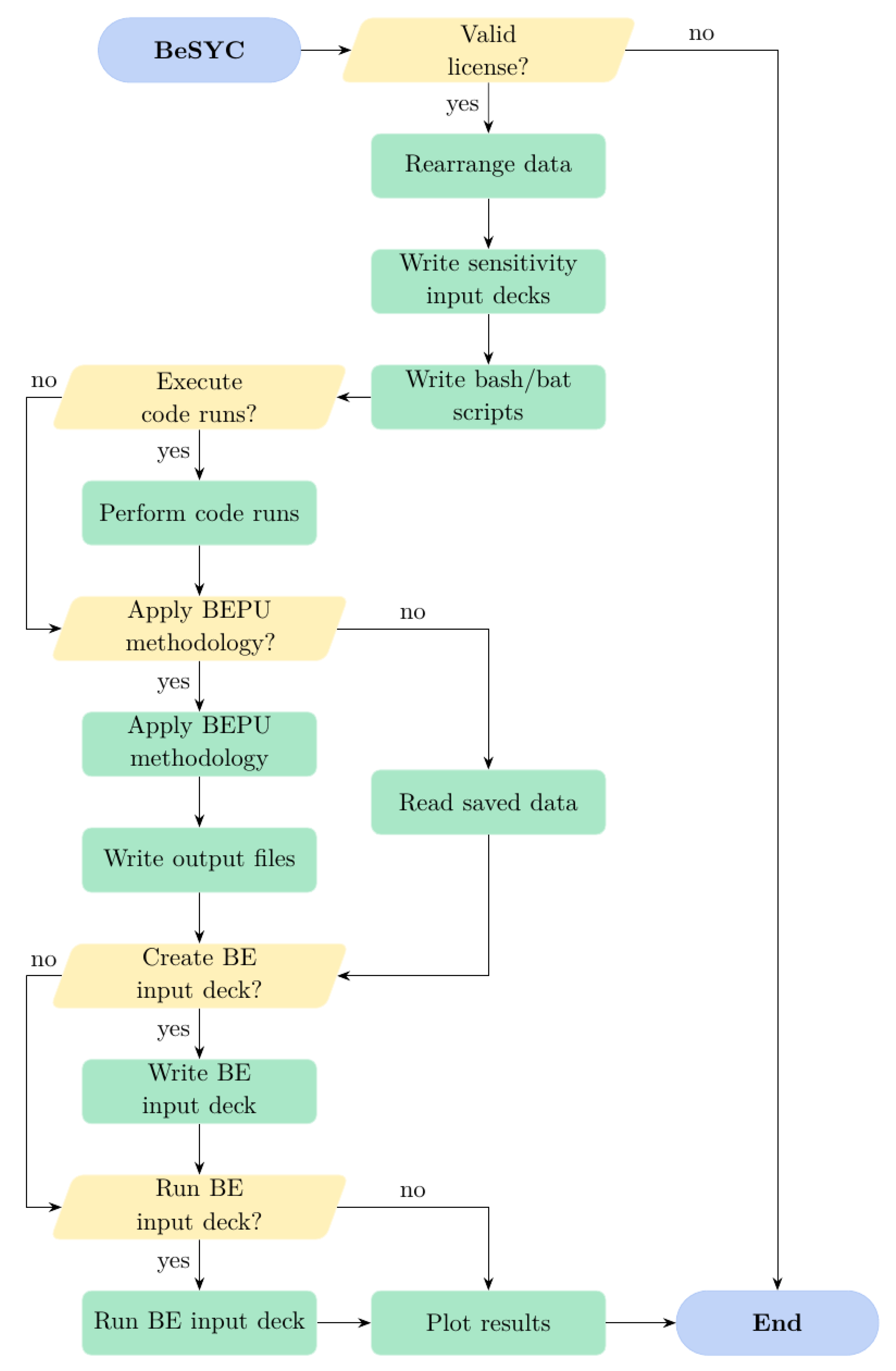The data required to run BeSYC are contained in an input file, but two additional files are always required: an input deck of the system code in use to reproduce the investigated experimental setup and a csv file containing the experimental data. BeSYC follows a quite linear structure (Figure 1) subdivided into eight phases:

• A preliminary check of the license to see if the computer is allowed to run the BeSYC software;
• A rearrangement phase to process the input data stored in the input file and to assess the code input deck and the experimental csv file. Error messages are thrown if errors are found in the data provided.
• A phase in which the required sensitivity input decks are created. An output file is also created during this phase to list the investigated parameters and the values used in the sensitivity code runs.
• An optional fourth phase in which the sensitivity code runs are executed. The code runs are performed through the use of bash/batch files depending on the adopted platform. BeSYC starts a new calculation when a previous one is over following the maximum number of parallel code runs (RELAP5-3D, MELCOR 1.8.6, and MELCOR 2.2 codes are single thread applications) defined by the user in the input file. Before starting the execution of the code runs, a check is also performed to ensure that number of parallel runs is smaller than the number of CPU threads to avoid system unresponsiveness. The status of the different code runs is not performed through MATLAB commands but through the pgrep (Linux) and the tasklist (Windows©) system commands. This phase is also optional because the eventual modification of the BEPU methodology input data do not usually require the re-execution of such code runs.
• A fifth optional phase devoted to the application of BEPU methodology and the creation of the output files summarizing the main findings. In this phase, the Pearson’s, Spearman’s and Kendall’s coefficient are also calculated. If the BEPU methodology is not applied, the results of a previous run are loaded (if available) to safely prosecute through the next phases.
• A sixth phase in charge of writing a best-estimate input deck (if requested).
• An optional seventh phase to run the best-estimate input deck (if requested).
• A final eighth phase to plot the comparison between the responses and their standard deviation in the experimental file, the default run, the BEPU methodology, and the BE run (if available).

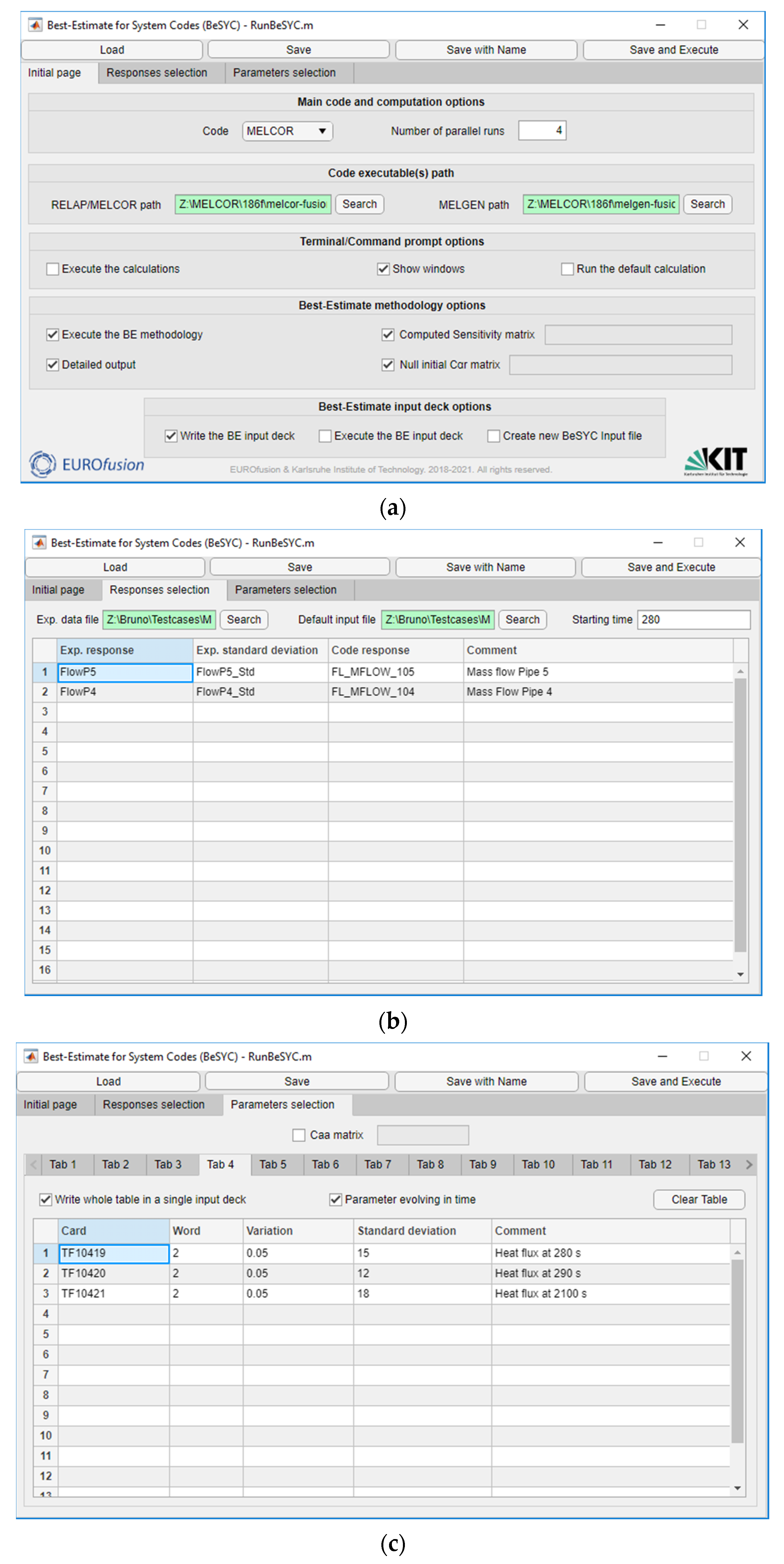
The data required to run the BeSYC app must follow a quite strict organization, so a GUI was created to ease this process (Figure 2). The GUI was developed with App Designer [14], and it works seamlessly with the scripts composing the BeSYC software. The four buttons at the top of the GUI can be used to load and save BeSYC input files as well as to run the BeSYC software. Below these buttons, the interface is divided into three main panels: the main panel (Figure 2a) in which most of the options are set, the responses panel (Figure 2b) dealing with the aspects concerning the responses, and the parameters panel (Figure 2c) hosting the data related to the parameters. The main panel is divided into five sections:

• The computational options to select the code and the number of parallel code runs if the execution of the calculation is requested;
• The code executables section to provide the path to the code’s executable(s);
• The Terminal/Command prompt section used to select if the code runs have to be executed (“Execute the calculations” and the “Run the default calculation” check boxes), and, if so, if the terminal/command windows should appear on the screen or if the calculations have to be performed in background;
• The best-estimate methodology section where the execution of the BEPU methodology and the verbosity of the output files can be selected. In this panel, it is also possible to select sensitivity and $C_{\alpha r}$ matrices taken from csv files.
• The best-estimate input deck section to specify if a best-estimate input deck has to be written and executed. In this section, is also possible to specify the creation of a new BeSYC input file containing the best-estimate standard deviation values.

The responses panel presents only four main elements: the paths to the experimental data file and the default input deck, the calculation time (starting time) from which the BEPU methodology is applied, and a table that is used to select the experimental and computed responses to be used in the BEPU methodology. Starting time is expressed in seconds, and it is used to skip the initial phase of a calculation that might be necessary to reach a steady state.

The parameters panel presents two main sections: a top section to select a $C_{\alpha \alpha }$ matrix from a csv file and a bottom section to define which parameters should be investigated together with their standard deviation and variation (in percentage) in the input decks. For both codes, each parameter can be selected, specifying the card and the word in which they appear, as described in the RELAP5-3D, MELCOR 1.8.6, and MELCOR 2.2 User’s Manuals [15,16,17]. The parameters are defined into several independent tables contained in different panels (Tab 1, Tab 2, etc.), each provided with two check boxes to state if the variations of the parameters specified in the current table should be written into a single input deck or not and, if yes, if they belong to a parameter evolving in time.

4. Verification and Validation

The verification and validation (V&V) of the BeSYC software followed a pragmatic approach to ensure the proper execution of all the scripts in each scenario. The V&V is eased by the independent nature of the BeSYC software. Indeed, given the fact that the software runs independently from the system codes, the original validation done by the RELAP5-3D and MELCOR 1.8.6 developer holds also in conjunction with the BeSYC software.

The V&V activity was divided into two parts: the V&V of the ancillary scripts, i.e., those not involved in the application of the numerical framework, and the V&V of the script applying the numerical framework. For the scripts in charge of writing textual file, the sole verification was sufficient to assess their correctness (scripts to write input decks, bash/bat files, and output reports). In this frame, it was noticed how the parameters having a default value of 0 cannot be used in the best-estimate methodology because the variation in terms of percentage would results in two sensitivity input decks identical to the default one. This limitation is not really correlated with BeSYC, but it derives from the brute force method adopted to calculate the sensitivities [10].

Instead, more demanding efforts were required to verify and validate the scripts to run the calculations and apply the mathematical framework. The script to run the calculations must ensure a good compromise between dead times (time between the end of a calculation and the start of a new one) and the correct handling of the code runs. The testing of this script was mostly done while testing the script to apply the mathematical framework. Three different checks were performed on this last script:

• A V&V against the examples provided in [18] to demonstrate the correctness in the implementation of the mathematical framework;
• A check for the Pearson, Spearman’s, and Kendall’s tau correlation coefficients against the results of the MATLAB built-in corr function [19]. This function is available in the Statistics Toolbox, but it is not used in BeSYC to avoid any dependency with optional MATLAB toolboxes.
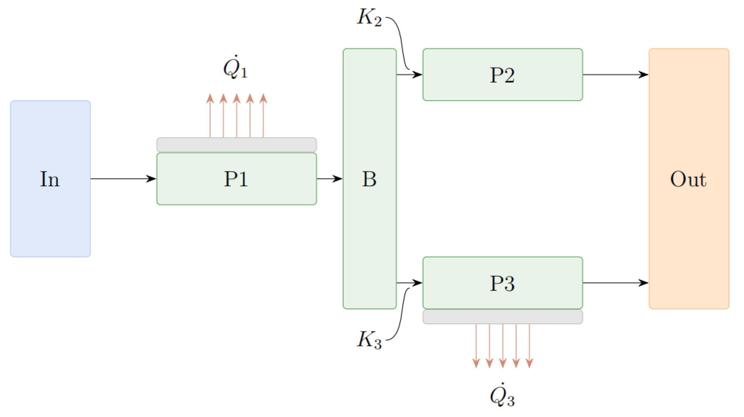
• A V&V against hand-made test cases to test the correct handling of the different input data that can be used as input for BeSYC (non-null $C_{\alpha r}$ matrix, a $C_{\alpha \alpha }$ matrix instead of the parameter’s standard deviation, and a sensitivity matrix instead of the use of the brute-force method). The results of these test cases have been cross-checked through hand calculations. The geometry of the test cases (Figure 3) consists in three pipes (P1, P2, and P3) connected through a branch (B). Two pipes (P1 and P3) are equipped with a heat structure characterized by a heat flux boundary condition on the external side. The mass flow rate through the system is established imposing different pressures in the In (8.01 MPa) and the Out (7.95 MPa) volumes. The three pipes have a length of 0.1 m, while the branch is 1-m long. The flow area of both the pipes and the branch is 1 m².

The test matrix consisted of 11 tests: (

Table 1. Test cases matrix.

Name	Parameters	Responses	Notes
1 Resp 1 Par	K3	Mass flow in J3	Single time node
1 Resp 2 Par	K3, ε	Mass flow in J3	Single time node
2 Resp 3 Par	K2, K3, ε	Mass flow in J2 and J3	Single time node
Time	K2, K3, ε	Mass flow in J2 and J3	Three time nodes
TPE (Time-Parameter-Evolve)	K2, K3, ε, $\dot{Q_3}$	Mass flow in J2 and J3	Three time nodes
TPE $C_{\alpha \alpha }$ full	K2, K3, ε, $\dot{Q_3}$	Mass flow in J2 and J3	As TPE plus a full size $C_{\alpha \alpha }$ matrix
TPE $C_{\alpha \alpha }$ single	K2, K3, ε, $\dot{Q_3}$	Mass flow in J2 and J3	As TPE plus a single block $C_{\alpha \alpha }$ matrix
TPE $C_{\alpha r}$ full	K2, K3, ε, $\dot{Q_3}$	Mass flow in J2 and J3	As TPE plus a full size $C_{\alpha r}$ matrix
TPE $C_{\alpha r}$ single	K2, K3, ε, $\dot{Q_3}$	Mass flow in J2 and J3	As TPE plus a single block $C_{\alpha r}$ matrix
TPE Sens full	K2, K3, ε, $\dot{Q_3}$	Mass flow in J2 and J3	As TPE plus a full size sensitivity matrix
TPE Sens single	K2, K3, ε, $\dot{Q_3}$	Mass flow in J2 and J3	As TPE plus a single block sensitivity matrix

): five tests to investigate the behavior with different types of parameters and responses and six to investigate the non-default BeSYC options. The typical responses adopted in these tests are the mass flow rates through the junctions that connect P2 and P3 pipes with the Out volume (J2 and J3, respectively). Instead, the parameters of the system are:

• The concentrated pressure drop coefficients (K2 and K3) between the branch and the two P2 and P3 pipes (parameters requiring the variation of a single input datum in the input deck);
• The surface roughness (ε) of the three pipes and the branch (parameter requiring the variation of more than one input datum in the input decks);
• The heat flow ($\dot{Q_3}$) from the heat structure connected to P3 (parameter changing in time).

The system was simulated in RELAP5-3D by means of pipe components (P1, P2, and P3) and a branch (B). The three pipe components are characterized by 10 equally sized nodes. Similarly, the heat structures are assumed composed by 10 nodes and by the thickness divided into five meshes. Instead, in MELCOR 1.8.6 and 2.2, the three pipes and the branch are reproduced with four independent volumes, and the heat structures have only three meshes along the 5-mm thickness.

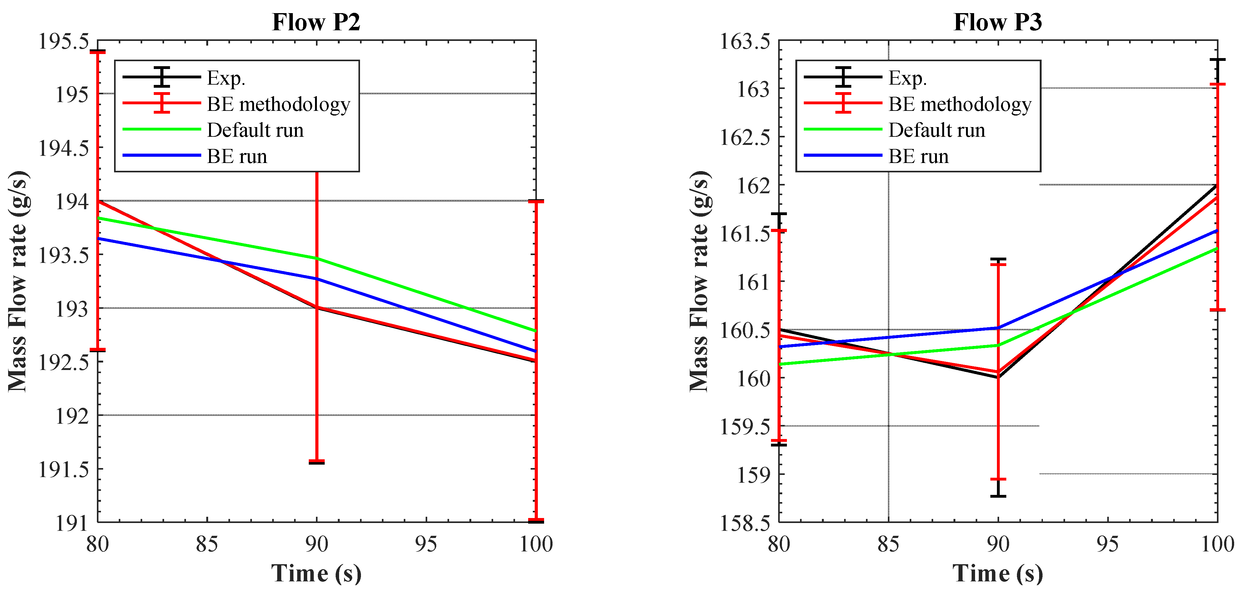
Figure 4 presents an overview of the achieved results in the TPE case for the RELAP5-3D code. This test was chosen, as it is the most usual utilization of the software. The two graphs in Figure 4 present four curves each: fictitious experimental data (black curve), best-estimate results obtained from the application of the best-estimate methodology (red curve), results of the default RELAP5-3D input deck (green curve), and results of the best-estimate RELAP5-3D input deck, i.e., an input deck adopting the best-estimated values of the parameters obtained from the methodology (blue curve). The good match between the best-estimate methodology results (red curve) and the fictitious experimental data supports the proper implementation of the methodology in the software. This conclusion is also supported by the smaller uncertainty of the best-estimate methodology results compared to that of the fictitious experimental data.

Instead, the discrepancy between the best-estimate methodology results (red curve) and the best-estimate RELAP5-3D code results (blue curve) is due to the fact that the methodology predicts different best-estimated values for the various parameters at each time node, but usually only a single value can be used in the input decks of the system/thermal-hydraulics codes, such as RELAP5-3D and MELCOR. If only a value has to be used, the most straightforward way to define one is to calculate an average best-estimated value basing on those obtained from the methodology. Hence, the discrepancy between the two curves is a direct effect of this simplification.

Nonetheless, in few specific scenarios, an additional source of discrepancy can arise from the usage of linearized sensitivity terms (Equation (5)). Depending on the scenario and on the model considered, one or more parameters may have an influence straying from linearity. In these cases, an iterative process (several calibrations one after another) may be required to reach a good agreement between experimental and computed results [4]. Nevertheless, this is not the case of the simple cases studied for the V&V of the BeSYC software.

The results of the different test cases were also benchmarked against hand-made calculations. The mean difference between the elements of the best-estimate vectors and matrices was in the order of 10⁻¹⁶ even if for some elements of the best-estimate parameters vector, the difference stood up to 10⁻⁸. In any case, these differences are sufficiently small to be neglected. This further suggests the correct implementation of the logics and the several options offered by the BeSYC software.

5. Application to Real-Case Scenarios

After the V&V, the BeSYC software has been applied to several real-case scenarios. In the first scenario, the BeSYC software was applied against several pressure drop characterization tests performed on a first wall mock-up [20]. This mock-up is a P92 steel plate crossed by 10 channels having a 15 mm × 15 mm square section. The characterization tests were performed to investigate the pressure losses across them thanks to the injection of air at 20 °C and ~6 bar. A calibration considering four parameters and one response was performed to reproduce these tests. The four parameters are the channel surface roughness and the three concentrated pressure drop coefficients at the geometrical discontinuities within the channel. Instead, the response is the differential pressure between the inlet and the outlet of the channel.

Figure 5 shows the results achieved from the application of the best-estimate methodology against the tests performed for two channels of the first wall mock-up (MELCOR 1.8.6 code, see [9] for further details). The analysis was mostly performed to demonstrate that the best-estimate input deck (blue curve) was capable to better reproduce the experimental trends compared to the default input deck (red curve) considered as starting point of the analysis. As it can be depicted from the two graphs, the goals of the analysis were achieved since the blue curve was much closer to the experimental results (black curve) than the red one. The differences between the results obtained from the best-estimate methodology and those of the best-estimate code run are again correlated to the necessity to use single values for the different parameter in the system/thermal-hydraulics codes.

Then, the BeSYC software was used for the post-test analysis with RELAP5-3D and MELCOR 1.8.6 of a LOFA experimental campaign performed in the KIT HELOKA-HP facility [8,9]. For this analysis, 10 responses and about 100 parameters were selected to reproduce the different experimental scenarios (11 tests). The BeSYC software was in charge to write the input decks, control their execution (about 200 code runs for each of the 11 tests), apply the best-estimate methodology, write the best-estimate input deck, and execute it. Moreover, in these scenarios (not discussed here for sake of brevity), the software demonstrated its capabilities when dealing with the different aspects of the analysis. Further information on the LOFA experimental campaign and the post-test analysis performed with BeSYC and the RELAP5-3D code can be found in [8], while the post-test analysis with BeSYC and the MELCOR 1.8.6 code are described in [9].

6. Conclusions

This work presents the efforts of KIT to develop and validate a software aimed at applying the best-estimate methodology discussed in [4,5]. This rigorous methodology is based on the Bayes’ theorem in conjunction with the information theory to assimilate the uncertainty-afflicted experimental and computational data. The purpose of the best-estimate methodology is to provide best-estimate/calibrated values of the parameters used to describe the physical systems, the responses, and their uncertainty used to describe the physical systems.

The tool, called BeSYC, is an interactive MATLAB App equipped with a GUI. The software was developed in the frame of the KIT activities devoted to the validation of system codes (RELAP5-3D and MELCOR 1.8.6) against data gathered from the experimental campaigns performed in the HELOKA-HP facility [8]. The development of BeSYC was grounded on three fundamental aspects:

• Independency from the system code in use;
• Modularity to ease the maintenance of the tool as well as to ease the introduction of new features or the support of new system codes;
• Multi-platform availability.

The tool has been extensively validated against both examples provided in literature and hand-made test cases. Then, BeSYC was used for the analysis of several pressure drop characterization tests and a LOFA experimental campaign performed on a helium-cooled first wall mock-up in the KIT HELOKA-HP facility [8,9]. These two works do not only represent the validation of the RELAP5-3D and MELCOR 1.8.6 codes in DEMO relevant conditions but also the last validation step of the BeSYC software. The findings of these latest activities pushed to introduce the support to the MELCOR 2.2 system code (not yet applied to any real-case scenario). The aim was to turn the BeSYC software in a simple yet powerful tool to perform BEPU studies. The use of a GUI without the prior knowledge of any programming language (Python, C++, etc.) also eases the introduction of young scientist/students to BEPU topics.