Review of Visual Saliency Prediction: Development Process from Neurobiological Basis to Deep Models

Abstract

The human attention mechanism can be understood and simulated by closely associating the saliency prediction task to neuroscience and psychology. Furthermore, saliency prediction is widely used in computer vision and interdisciplinary subjects. In recent years, with the rapid development of deep learning, deep models have made amazing achievements in saliency prediction. Deep learning models can automatically learn features, thus solving many drawbacks of the classic models, such as handcrafted features and task settings, among others. Nevertheless, the deep models still have some limitations, for example in tasks involving multi-modality and semantic understanding. This study focuses on summarizing the relevant achievements in the field of saliency prediction, including the early neurological and psychological mechanisms and the guiding role of classic models, followed by the development process and data comparison of classic and deep saliency prediction models. This study also discusses the relationship between the model and human vision, as well as the factors that cause the semantic gaps, the influences of attention in cognitive research, the limitations of the saliency model, and the emerging applications, to provide new saliency predictions for follow-up work and the necessary help and advice.

1. Introduction

Approximately 80% of the information that humans receive every day comes from vision. However, human visual nerve resources are limited [1]. An information bottleneck exists in the human visual pathway. For instance, the visual system receives hundreds of megabytes of visual media data every second, but the information processing speed is only 40 bits per second [2]. In this process, the visual attention mechanism plays an important role [3]. Among the information received in our daily lives, only a small amount of stimuli can enter the visual system for further processing at any time, thereby avoiding computational waste and reducing the difficulty of analysis. The development of the Internet and the popularization of smart devices have enhanced the speed of information collection and dissemination, even reaching an unprecedented level. However, if all information is indiscriminately allocated with the same computing resources, then it will lead to a waste of computing resources and excessive time consumption. Knowing how to select interesting content from massive scenes for analysis and processing in the same way as human beings is therefore a very important endeavor.

Visual saliency prediction is a mechanism that imitates human visual attention, including relevant knowledge such as neurobiological, psychological, and computer vision. Early attention models often used cognitive psychological knowledge to find information about behaviors, tasks, or goals. For example, Itti et al. [4] proposed a saliency prediction model based on the bottom-up model, from which the deep learning models have gradually flourished. Compared with the classic models, the performance of these newly developed models has been greatly improved, and the performance is gradually approaching the human inter-observer. The significance of the research on visual saliency detection lies in two aspects: first, as a verifiable prediction, it can be used as a model-based hypothesis test to understand human attention mechanisms at the behavioral and neural levels. Second, the saliency prediction model based on the attention mechanism has been widely used in numerous ways, such as target prediction [4], target tracking [5], image segmentation [6], image classification [7], image stitching [8], video surveillance [9], image or video compression [10], image or video retrieval [11], salient object detection [12], video segmentation [13], image cropping [14], visual SLAM (Simultaneous Localization and Mapping) [15], end-to-end driving [16], video question answering [17], medical diagnosis [18], health monitoring [19] and so on.

The current research on saliency detection mainly involves two types of tasks, namely, saliency prediction (or eye fixation prediction) and Salient Object Detection (SOD). Both types of tasks aim to detect the most significant area of a picture or a video. However, differences exist between these two models and their application scenarios. Saliency prediction is informed by the human visual attention mechanism and predicts the possibility of the human eyes to stay in a certain position in the scene. By contrast, salient object detection, as the other branch, focuses on the perception and description of the object level, which is a pure computer vision task. The two types of tasks asre shown in Figure 1.

Numerous researchers have recently investigated SOD tasks. Presumably, as a pure visual task, SOD can be more easily and directly applied to certain visual scenes, which is more driven by applications in different fields. Benefiting from large-scale benchmarking and deep learning, SOD has been developing rapidly and has shown amazing achievements [20]. In recent years, many researchers have made outstanding contributions. Wang et al. [21] proposed a general framework using iterative top-down and bottom-up saliency inference. In addition, the framework used parameter sharing and weight sharing to reduce the amount of parameters. Besides, Wang et al. [22] proposed the PAGE-Net, which mainly included two modules: pyramid attention and salient edge detection. With an enlarged receptive field, PAGE-Net obtained the edge information by predicting the edge of significant objects through supervised learning. The model proposed by Zhang et al. [23] applied joint training to the two almost opposite tasks of SOD and COD(Camouflaged Object Detection). The Dual ReFinement Network (DRFNet) proposed by Zhang et al. [24] can be directly applied to high-resolution images. DRFNet consisted of a shared feature extractor and two effective refinement heads, which could obtain more discriminative features from high-resolution images.

However, the salient object is not necessarily the only possible salient target in the graph. Other complicated factors should be considered. In addition to its wide range of applications, the saliency prediction task is related to human vision itself, and it is closely related to neuroscience and psychology. Consequently, saliency prediction has been widely used in interdisciplinary and emerging subjects. The main contributions of this study are as follows:

• This research focused on the task of saliency prediction, analyzed the psychological and physiological mechanisms related to saliency prediction, introduced the classic models that have been affected by saliency prediction, and determined the impact of these theories on deep learning models.
• The visual saliency model based on deep learning was analyzed in detail, and the performance evaluation measures of the representative experimental datasets and the model under static and dynamic conditions were discussed and summarized, respectively.
• The limitations of the current deep learning model were analyzed, the possible directions for improvement were proposed, new application areas based on the latest progress of deep learning were discussed, and the contribution and significance of saliency prediction with respect to future development trends were presented.

2. Psychological and Neurobiological Basis of Visual Saliency

Attention mechanism has always been an important subject of neuroscience and psychology. In the mid-1950s, cognitive psychology gradually emerged. Attention was regarded as an important mechanism of human brain information processing, and several influential attention models, such as the filter model (1958), attenuation model (1960), and response selection model (1963), among others, were produced. Treisman [25] proposed an important model called Feature Integration Theory (FIT) to vividly illustrate the selective role of visual attention. The visual process in this model was divided into a pre-attention stage and a focal attention stage. Feature integration was implemented after extracting the location-related features. Koch and Ullman [26] enhanced FIT by integrating the return-inhibition mechanism to achieve a focus shift. Moreover, on the basis of criticisms of the early FIT model, Wolfe [27] proposed the guided search model to explain and predict search results. These neurological and psychological studies have provided an important basis and criteria for calculating visual saliency, such as center surround antagonism, global rarity, or maximization of information.

Visual saliency prediction mainly used mathematical models to simulate the human visual attention function and subsequently calculated the importance of visual information. The simulation of the human visual attention system mainly used some of the important achievements in visual physiology and psychology mentioned above. Notably, visual saliency prediction did not study eye movement strategies in visual attention but rather calculates the information pertaining to the different degrees of importance with respect to scenes for eye movement decision-making. These studies have played a guiding and standardizing role in the subsequent development of saliency detection models.

3. Classic Visual Saliency Models

The classic visual saliency model considered the psychological and neurobiological basis, and most of them were handcrafted feature models. As a research basis of psychology, classic visual saliency models could be usually divided into two models according to the level of information processing: bottom-up saliency models (data-driven, task-agnostic model), and top-down saliency models (task-driven, task-specific model).

3.1. Bottom-Up Visual Saliency Models

Bottom-up visual saliency models usually extract low-level features, such as contrast, color, and texture. The difference between low-level features and background features strongly attract attention resources. This attention prediction mechanism is involuntary and entails fast processing. For example, the presence of pedestrians, vehicles, individual flowers, and beasts in an image will show strong visual saliency. Among them, the local contrast model is based on the physiological and psychological principles of FIT and the center surround antagonism, and it defines a certain mechanism when selecting salient areas in an image to realize the simulation of the visual attention mechanism. For example, the earliest model of Itti [4] could simulate the process of shifting human visual attention without any prior information. According to the features captured from images, the model analyzed visual stimuli, allocated computing resources, selected the salient areas in the scene according to the saliency intensity of different positions, and simulated the process of human visual attention transfer. Although the performance of the model was general, it was the first successful attempt from the neurobiological model, which is of great significance. Since then, other researchers have contributed improvements. Harel [28] changed the graph-based visual saliency (GBVS) model to the Markov random field with non-linear combination in the synthesis stage. The model formed activation maps on certain feature channels, and then normalized them in a way which highlighted conspicuity and admitted combination with other maps. Ma and Zhang [29] used local contrast analysis to extract the saliency maps of an image, and on this basis, Tie Liu et al. [30] used 9 × 9 neighborhoods and adopted a conditional random field (CRF) learning model. Borji [31] analyzed local rarity based on the sparse coding. Sclaroff et al. [32] proposed a saliency prediction model based on Boolean Map. In addition, researchers have used other models to predict saliency by using local or global contrast. Some of the notable examples include the pixel-level contrast saliency model proposed by Zhai and Shah [33], the sliding windows-based model for global contrast calculation proposed by Wei [34], the color contrast linear fusion model proposed by Margolin [35], the frequency tuning model proposed by Achanta [36], and the color space quantization model proposed by Cheng [37]. Other researchers have used the superpixel [38,39,40] as the processing unit to calculate the variance of color space distribution as a means of improving the computational efficiency.

Some models have been based on information theory and image transformation. The essence of these models based on information theory is to calculate the maximum information sampling from the visual environment, select the richest part from the scene, and discard the remaining part. Among them, the Attention-based on Information Maximization (AIM) model of Bruce and Tsotsos [41] was influential. The AIM model has used Shannon’s self-information measure to calculate the saliency of the image. Firstly, a certain number of natural image blocks were randomly selected for training to obtain the basic function. Then, the image was divided into blocks of the same size, the basis coefficients of the corresponding blocks were extracted as the features of the block through Independent Component Analysis (ICA), the distribution of each feature was obtained through probability density estimation, and finally the probability density of the feature was obtained. Other notable models included the incremental coding length model proposed by Hou [42], the rare linear combination model proposed by Mancas [43], the self-similarity prediction model proposed by Seo [44] and the Mahalanobis distance calculation model proposed by Rosenholtz [45]. As for the use of image transformation models for saliency prediction, the spectral residual model proposed by Hou [46] did not examine the foreground characteristics but rather utilizes the research background. The areas that did not match these features are the areas of interest. After calculating the residual spectrum, the residual spectrum was mapped back to the spatial domain by inverse Fourier transform to obtain the saliency map. On this basis, Guo [47] proposed a model that used the phase spectrum to obtain the saliency map and Holtzman-Gazit [48] extracted a variety of resolutions for the picture. Sclaroff [49] proposed a Boolean Map based saliency model(BMS) by discovering surrounding regions via boolean maps. The model obtained saliency maps by analyzing the topological structure of boolean maps. Although BMS was simple to implement and efficient to run, it performed well in the classical models.

3.2. Top-Down Visual Saliency Models

The top-down visual saliency model is often based on certain specific tasks. Due to the diversity and complexity of tasks, modeling is also more difficult [50]. The top-down visual saliency model is mainly based on the Bayesian model. In addition, the Bayesian model can be regarded as a special case of the decision theoretical model, as both simulate the biological calculation process of human visual saliency.

The Bayesian model in saliency prediction is a probabilistic combination model that combined scene information and prior information according to Bayesian rules. The model proposed by Torrallba et al. [51] multiplied the bottom-up and top-down saliency maps to obtain the final saliency map. On this basis, Ehinger et al. [52] integrated the feature prior information of the target into the above framework. Xie et al. [53] proposed a saliency prediction model based on posterior probability. The SUN model proposed by Zhang et al. [54] used visual features and spatial location as the prior knowledge.

The model based on decision theory in saliency prediction is a strategy model that decides the optimal plan based on the information and evaluation criteria requirements, i.e., how to make optimal decisions about perceptual information of the surrounding environment. Gao and Vasconcelos [55,56] believe that the salient features in the recognition process are derived from other classes of interest, and they defined top-down attention as a classification problem with the smallest expected error. Kim et al. [57] recommended a temporal and spatial saliency model based on motion perception grouping. Gu et al. [58] proposed a model based on the decision theory mechanism to predict regions of interest.

Early machine learning models often use a variety of machine learning methods, such as Convolutional Neural Networks (CNNs), Support Vector Machines (SVMs), or probability kernel density estimation, and they mostly combined the bottom-up and top-down methods. Notable examples included the nonlinear mapping model proposed by Kienzle et al. [59], the regression classifier model proposed by Peters et al. [60], and the linear SVM model proposed by Judd et al. [61]. Those early machine learning models had a certain exploratory nature for subsequent deep learning models, and they played an important guiding role for the subsequently developed deep learning models.

Although these classical models were designed in a variety of ways, their performance gradually reached a bottleneck due to handcrafted features. The development process of neurobiological models and classic models is shown in Figure 2.

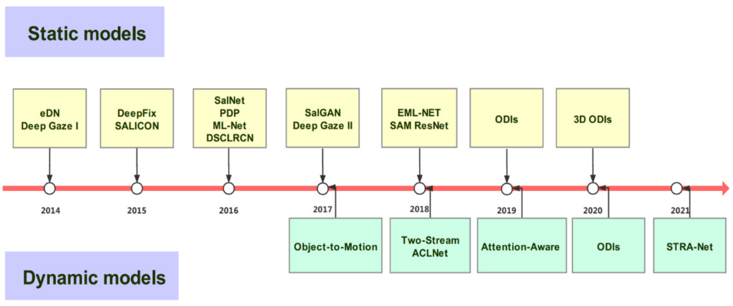
4. Deep Visual Saliency Models

In 2014, Vig et al. [62] proposed a deep convolutional network named eDN that could be implemented in fully automatic data-driven mode to extract features. Compared with the classic model, eDN could automatically learn the image expression and obtain the final saliency map by fusing the feature maps from different layers. However, due to the limited number of datasets and the limited number of trainable graphs in the data set, the depth of the network was not enough, as the structural scalability was limited. Since then, more researchers have used deep models to study saliency prediction, and the application of deep models in static and dynamic saliency prediction has achieved better results.

4.1. Static Models

After eDN, Kümmerer et al. [63] proposed a CNN model named Deep Gaze I based on image classification by using the AlexNet [64] network. The major innovation of Deep Gaze I was the application of transfer learning for saliency prediction by using pre-trained weights on ImageNet [65], connecting them to the output layer of AlexNet. The network contains a central deviation that was converted into a probability distribution by using a softmax function. The typical saliency datasets were relatively small, and the training effect was limited. ImageNet has a good training effect as a million-level database, but the training resources are huge and the training time is excessive. The use of transfer learning based on ImageNet makes it easier to learn the features of deep CNNs (DCNN) and attain much better generalization effects. Kruthiventi et al. [66] proposed the DeepFix model in the same year, by using the VGG-16 [67] network as the main feature extraction network, allowing the network to use location-related information. Compared with AlexNet, the VGG-16 network is simpler and more effective. Using a better target prediction network becomes a better choice. Then, DeepGaze II [68] switched to VGG-19 [67], retrained the image features on the SALICON [69] dataset, and then fine-tuned on the MIT1003 [70] dataset. As a result, the performance of the updated model has been significantly improved compared with that of Deep Gaze I. This development trend indicated that retraining deep features and the task of fine-tuning contribute to performance enhancement. Many researchers have adopted small-scale retraining and fine-tuning with the successful use of transfer learning.

Similarly, many researchers have adopted models that can capture relatively fine or coarse features by adjusting the input of different resolutions as a means of achieving better results. Among them, Pan et al. [71] proposed two saliency models: shallow ConvNet (JuntingNet) and deep ConvNet (SalNet) to train end-to-end architectures. SALICON was used to train a convolutional network by using VGG-16 network with dual-branch multi-scale features. Dual-branch can effectively improve the model performance, but the calculation cost and memory are higher in training and testing.

Then, by combining migration-integrating information on different image scales, the model could greatly surpass the level of advancements at the time. The probability distribution prediction model proposed by Jetley et al. [72] defined saliency as a generalized Bernoulli distribution, and it included a fully end-to-end training deep CNN that combined the classic softmax loss with the calculation of the different probability distributions. Their results showed that the new loss function was more effective than the classic loss function (e.g., Euclidean) in saliency prediction. Liu and Han [73] proposed a Deep Spatial Contextual Long-Term Recurrent Convolutional Network (DSCLRCN) model. First, CNN was used to learn the local saliency of small image regions, and then images in the horizontal and vertical directions were scanned using the Long Short-Term Memory networks (LSTMs) to capture the global context. These two operations allowed DSCLRCN to effectively merge local and global contexts at the same time for inferring the saliency maps of the image.

The ML-Net model proposed by Cornia et al. [74] combined the advantages of the above models. Their model consisted of a feature extraction DCNN, a feature coding network, and an a priori learning network. At the same time, the loss function of the network was weighted by three parts: NSS, CC, and SIM. The SALICON model also used differentiable metrics, such as NSS, CC, SIM, and KL divergence, to train the network. The SAM-ResNet model and SAM-VGG model subsequently proposed by Cornia et al. [75] combined the full convolutional network and the cyclic convolutional network to obtain a spatial attention mechanism. SalGAN [76] used adversarial networks for training, and it consisted of two parts, a generator and a discriminator. The network learned the parameters through the backpropagation of the downsampled binary cross entropy loss calculation. The success of the model indicated that the choice of an appropriate loss function can be treated as a method for improving the prediction effect.

In recent years, some excellent models have been proposed for saliency prediction. Jia et al. [77] proposed a saliency model called EML-Net based on the similarities between images and the integration of Extreme Learning Machines (ELMs). Wang et al. [78] proposed the Deep Visual Attention (DVA) model in which the architecture was trained in multiple scales to predict pixel saliency based on a skip-layer network. The model proposed by Gorji [79] used shared attention to enhance saliency prediction. Dodge et al. [80] proposed a model called MxSalNet, which was formulated as a mixture of experts. Mahdi et al. [81] proposed a deep feature-based saliency (DeepFeat) model to utilize features by combining bottom-up and top-down saliency maps. AKa et al. [82] proposed the MSI-Net based on an encoder–decoder structure and it includes a module with multiple convolutional layers at different dilation rates to capture multi-scale features.

4.2. Dynamic Models

Unlike the settings of the static models, the observation time in dynamic models is reduced from approximately 4 s to 0.05 s. In addition, due to the obvious motion information in videos, predicting the saliency of the dynamic video is more difficult. As a result, much fewer dynamic models exist. Nevertheless, as the demand for applications continues to grow, the research on dynamic models has also been continuously developing.

Dynamic models usually add temporal information to CNNs or use LSTMs for modeling. Early dynamic models mainly combined static saliency features with temporal information based on the bottom-up model. Gao et al. [83] integrated additional motion information, and Seo et al. [84] used a local regression kernel to calculate the similarity between the pixels in the video and its surrounding area. However, the performance of these models were restricted by their handcrafted features. The emergence of deep learning frameworks has improved this situation. Bak et al. [85] proposed the dynamic model and added motion features based on the two-stream network. Due to the final fusion of the information of the two streams, the network was limited in learning spatiotemporal features. Chaabouni et al. [86] added residual motion and RGB color planes of two consecutive frames to CNN based on transfer learning. The model of Leifman et al. [87] merged the RGB color planes, dense optical flow map, and saliency map into a seven-layer CNN network. Wang et al. [88] proposed a spatiotemporal residual attentive network (STRA-Net), which learned a stack of local attentions as well as global attention priors to filter out unrelated information. The model has advantages in precisely locating dynamic human fixations as well as capturing the temporal attention transitions.

LSTMs are also widely used in dynamic models. Bazzani et al. [89] used 3D CNNs to connect with the LSTMs and projected the output of the LSTMs to a Gaussian mixture model. The Object-to-Motion (OM)-CNN model proposed by Jiang et al. [90] analyzed intra-frame saliency based on the salient object networks and the motion information networks. On this basis, Gorji [91] proposed a multi-stream convolutional LSTM (ConvLSTM) network with three networks (gaze following, rapid scene change, and attention feedback) based on the static model. The ACLNet proposed by Wang et al. [92] used an enhanced CNN-LSTMs to encode static saliency information. However, the ability of the network to capture motion information was limited. In this manner, LSTMs can focus on learning temporal saliency representations across consecutive frames and avoid overfitting. Hang et al. [93] designed an attention-aware ConvLSTM to obtain spatial features from static networks and temporal features from dynamic networks, subsequently integrating them. The features extracted from consecutive frames were used to predict the salient regions, and a final salient map is generated for each video frame.

In the past two years, the dynamic saliency field has gradually developed in the direction of omnidirectional images (ODIs) and 3D ODIs. Xu et al. [94] used adversarial networks to predict the saliency of ODIs by imitating the head trajectory of the object and applied generative adversarial simulation models to train deep models. The development process of saliency prediction models is shown in Figure 3.

5. Visual Saliency Prediction Datasets

Many databases for target detection and image segmentation can be used as experimental data; many of them have been obtained by eye-tracking devices and manual annotations. The performance of saliency maps generated by different saliency models needs to be quantitatively evaluated. At present, the application of visual saliency prediction is mainly conducted for images and videos. The corresponding databases are also divided into two types: static and dynamic.

5.1. Static Datasets

• TORONTO dataset: In 2006, Bruce et al. [41] established the TORONTO dataset. It is one of the earliest and most widely used datasets of computer vision. It includes 120 color images with a resolution of 511 × 681. The images contain indoor and outdoor scenes and a total of 20 recorded observers’ eye movement data.
• MIT300 dataset: In 2012, Judd et al. [70] of MIT established the MIT300 dataset. It contains 300 natural images from Flickr’s creation and sharing and the eye movement data of 39 observers. At that time, the MIT300 dataset was the most influential and most widely used in the dataset saliency field. The dataset is generally not used as a training set. However, the model comprising the MIT300 dataset can be evaluated.
• MIT1003 dataset: The MIT1003 dataset was also established by Judd et al. [61]. It contains a total of 1003 images from Flickr’s collection of images and the LabelMe website and the eye movement data of 15 observers. The MIT1003 dataset can be regarded as a supplement to the MIT300 dataset. The MIT1003 and MIT300 datasets can be used as a training set and a test set for performance evaluation, respectively.
• DUT-OMRON dataset: In 2013, Yang et al. [95] established the DUT-OMRON dataset. It contains 5168 images, and each image provides eye movement data of 5 observers. This dataset is annotated with eye movement data, but it mainly focuses on salient object detection, with one or more salient objects and a relatively complex background.
• CAT2000 dataset: The CAT2000 dataset was established by Borji et al. [96]. It contains 2000 images under free observation by 24 observers. Twenty scenes are categorized as cartoon, art, indoor, and outdoor scenes. These categories contain bottom-up attention cues and top-down factors. The different types of images are suitable for a variety of attention behavior studies.
• SALICON dataset: In 2015, Ming et al. [69] established the SALICON dataset. This large mouse tracking dataset for contextual saliency was established by selecting 20,000 images in MS-COCO. It is currently the largest attention dataset in terms of scale and context variability. The difference from the abovementioned databases is that the SALICON dataset does not use an eye tracker to record eye movement data but rather uses the Amazon Mechanical Turk platform; however, the eye movement data recorded by the mouse was used to evaluate the performance of the model. Tavakoli et al. [97] emphasized that problems may arise in evaluating model performance when eye movement data are recorded by the mouse. Nonetheless, the SALICON dataset is the largest dataset in the current field, and it continues to be widely used by current mainstream saliency prediction models based on deep learning technology. The SALICON dataset offers eye movement data for the training set (10,000 pictures) and validation set (5000 pictures), and it can retain the eye movement data of the test set (5000 pictures).
• EMOd dataset: The EMOd dataset is a new dataset proposed by Fan et al. [98]. It contains 1019 emotional images with target-level and image-level annotations. It was designed for studying visual saliency and image emotion. In the image labeling process of the EMOd dataset, the main target objects in each image are labeled with attributes, such as target contour, target name, emotional category (negative, neutral, or positive), and semantic category. The four semantic categories are as follows: the target directly related to humans, the target related to human non-visual perception, the target designed to attract attention or interact with humans, and the target with implicit signs. Each target is coded to have one or more categories. Furthermore, the EMOd dataset has a total of 4302 targets with fine contours, emotional labels, and semantic labels. The number of positive, neutral, and negative targets are 839, 2429, and 1034, respectively.

In these datasets, SALICON has the largest amount of data for static models. Most models could use transfer learning to fine-tune on SALICON. Mit300 and cat2000, as databases containing the most model comparisons, are usually used for model performance testing.

5.2. Dynamic Datasets

The discussion in Section 4.2 has established the particularities of dynamic information and human attention and the limitation of eye movement equipment, which have led to difficulties in observing dynamic data. Incidentally, owing to the growth of application requirements, some large datasets have emerged in recent years. At present, the dynamic dataset mainly consists of the following:

• DIEM dataset: The DIEM dataset was established in 2011 by Mital et al. [99]. It contains a total of 84 videos, including advertisements, movie trailers, and documentaries, among others. A total of 50 observers have provided eye movement data through free viewing. The scene content and data scale are both limited.
• UCF-sports dataset: The UCF-sports dataset was established by Mathe et al. [100]. The dataset contains 150 videos, including 9 common sports categories. Different from the DIEM dataset, the observation object in the UCF-sports dataset is prompted by time-based actions in the video during the viewing process. The result is found to be purposeful.
• Hollywood-2 dataset: The Hollywood-2 dataset was also established in 2012 by Mathe et al. [100]. The dataset contains 1770 videos that are labeled according to 12 action categories, such as eating and running, among others. Unlike the UCF-sports dataset, the observation objects of the Hollywood-2 dataset are divided into three groups: free viewing, human action annotation, and video content annotation. The human-eye focus data are in the free viewing mode only and accounts for a small proportion of all of the data.
• DHF1K dataset: The DHF1K dataset was established by Wang et al. [92] in 2018. The dataset consists of a total of 1000 video sequences watched by 17 observers and covers seven main categories and 150 scene sub-categories. The video contains 582,605 frames with a total duration of 19,420 s. The DHF1K dataset also provides calibration for movement mode and number of objects, among others, thus providing convenience for studying high-level information of the dynamic attention mechanism.
• LEDOV dataset: The LEDOV dataset [101] was established by Wang et al. in 2018. It includes daily activities, sports, social activities, art performances, and other content. A total of 538 videos, with a resolution of 720px, contain a total of 179,336 frames of video and 5,058,178 gaze locations.

For early dynamic models, the DIEM, Hollywood-2, and UCF-sports datasets were the three most widely used datasets in video saliency research. In recent years, with the continuous updating of datasets, there are more models also using the DHF1K database for training and testing. The DHF1K database has a huge amount of data and a wide range of application.

6. Evaluation Measures for Visual Saliency Prediction

The metrics of visual saliency prediction mostly use similarities and differences between estimated predicted values and the Ground Truth (GT) and then outputs an evaluation score to judge the similarity or difference degree between them. Given a set of true values used to define the scoring function, the saliency prediction map can be used as the input, and the result of evaluating the accuracy of the prediction is returned. The evaluation measures are as follows:

AUC variant: The Area Under Curve (AUC) is used as a measurement standard for the two-class pattern recognition problem. Different from the AUC in tasks, such as target detection and image segmentation, given the particularity of the saliency prediction task, the following AUC variants are often used in the saliency prediction tasks:

• AUC-Judd: Judd et al. [102] proposed a variant of the AUC called AUC-Judd. For a given threshold, the true-positive probability is the ratio of the pixels predicted as significant on all true-valued salient points, whereas the false-positive probability is the ratio of pixels predicted as significant on non-salient points.
• AUC-Borji: Borji et al. [103] proposed another variant of the AUC called AUC-Borji. This variant uses the uniform random sampling of non-focus points to calculate the false positive rate and defines the saliency mapping value above the threshold of these pixels as false positive. The false positive calculation in AUC-Borji is a discrete approximation of the calculation in AUC-Judd. Due to the use of random sampling, the same model may be evaluated with different results.
• Shuffled AUC: Shuffled AUC (sAUC) [97] is also a commonly used AUC variant. It reduces the sensitivity of the AUC to the center shift by sampling the salient point distribution of other images.

AUC-Judd, AUC-Borji, and sAUC, as variants of AUC, are widely used in the evaluation of saliency models. Their values are positively correlated with model performance. Although AUC is an important evaluation measure, it cannot distinguish the relative importance of different regions. Therefore, other distribution-based similarity evaluation measures are needed:

• Normalized Scanpath Saliency (NSS): NSS is a unique evaluation measure of saliency prediction. It is used to calculate the average normalized significance value at the point of interest [104]. The calculation formula of NSS is

$$\mathrm{NSS}=\frac{1}{\mathrm{N}}{{\displaystyle \sum }}_{\mathrm{i}=1}^{\mathrm{N}} \overline{\mathrm{P}}\left(\mathrm{i}\right)\times \mathrm{Q}\left(\mathrm{i}\right)$$

(1)

where $\overline{\mathrm{P}}$ is the average value at the gaze point Q of the human eye, N is the total number of human eye gazes, i represents the i-th pixel, and N is the total number of pixels at the gaze point. A positive NSS indicates consistency between mappings, whereas a negative NSS is the opposite. The NSS value is negatively correlated with model performance.

• Linear Correlation Coefficient (CC):The CC is the statistic used to measure the linear correlation between two random variables. For the significance prediction evaluation, the prediction significance map (P) and the true value view (G) can be regarded as the two random variables. The calculation formula of CC is

$$\mathrm{CC}=\frac{\mathrm{cov}\left(\mathrm{P},\mathrm{G}\right)}{\mathsf{\sigma }\left(\mathrm{P}\right)\times \mathsf{\sigma }\left(\mathrm{G}\right)}$$

(2)

where cov is the covariance, σ is the standard deviation. The CC can equally distinguish false positives and false negatives at the value range of (−1,1). A value close to the two ends indicates a better model performance.

• Earth Movers Distance (EMD): EMD [105] represents the distance between the two 2D maps denoted by G and S, and it calculates the minimum cost of converting the estimated probability distribution of the saliency map S into the probability distribution of the GT map denoted by G. Therefore, a low EMD corresponds to a high-quality saliency map. In saliency prediction, EMD represents the minimum cost of converting the probability distribution of the saliency map into human-eye attention maps called the fixation map.
• Kullback–Leibler (KL) Divergence: KL divergence is a general information theory measurement corresponding to the difference between two probability distributions. The calculation formula of KL is

$$\mathrm{KL}\left(\mathrm{P},\mathrm{G}\right)={{\displaystyle \sum }}_{\mathrm{i}}{\mathrm{G}}_{\mathrm{i}}\log (\mathsf{\epsilon }+\frac{\mathrm{G}}{\mathsf{\epsilon }+{\mathrm{P}}_{\mathrm{i}}})$$

(3)

Similar to other distribution-based measures, KL divergence takes the predicted saliency map (P) and the true value view (G) as the input and evaluates the loss of information where P is used to approximate G, ε is the regularization constant. Furthermore, KL divergence is an asymmetric dissimilarity measure. A low score indicates that the saliency map is close to the true value.

• (6) Similarity Metric (SIM): SIM measures the similarity between two distributions. After normalizing the input map, SIM is calculated as the sum of the minimum values at each pixel. The calculation formula of SIM is

$$\mathrm{SIM}\left(\mathrm{P},\mathrm{G}\right)={{\displaystyle \sum }}_{\mathrm{i}}\min ({\mathrm{P}}_{\mathrm{i}},{\mathrm{G}}_{\mathrm{i}})$$

(4)

Given the predicted significance map (P) and the true value view (G), a SIM of 1 means that the distribution is the same, whereas a SIM of 0 means no overlap. SIM can penalize predictions that fail to consider all true densities.

In general, these evaluation measures are complementary. A good model should be good under a variety of evaluation measures, because these measures reflect different aspects of the saliency map. Usually, a variety of evaluation measures are selected when evaluating the model. As a widely used measure of location based, AUC is essential. At the same time, a variety of other measures such as CC, SIM and other distribution-based measures should be selected to reflect other salient map factors such as relatively saliency region or similarity.

Thus far, we have summarized the abovementioned six common evaluation measures based on whether they are appropriate as probability distribution, similarity, and continuous GT tools for statistics and classification. The details are shown in

Table 1. Summary of evaluation measures for visual saliency prediction.

Evaluation Measures	Location Based	Distribution Based	Similarity	Continuous Ground-Truth
AUC-Judd	√	√	√	√
AUC-Borji	√		√
sAUC	√		√
EMD		√		√
NSS	√		√
CC		√	√	√
SIM		√	√	√
KL		√		√

.

7. Performance of Visual Saliency Prediction Models

The MIT benchmark has the most comprehensive saliency model and evaluation benchmark. In this chapter, the static image performance evaluation results of the models in the MIT300 and CAT2000 datasets are selected over the MIT benchmark. Then, the performance of the dynamic model is selected over the DHF1K dataset. The data have been obtained from the running results of the MIT benchmark, the author’s study, and the author’s program on GitHub.

The MIT benchmark has a total of eight evaluation measures (including three AUC variants). A total of 93 static models are evaluated. The following 16 models with much better performance are selected for comparison: eDN, Deep Gaze I, Deep Gaze II, DeepFix, SALICON, SalNet, ML-Net, SalGAN, EML-Net, SAM-VGG, SAM-ResNet, AIM, Judd Model, GBVS, ITTI, and SUN. In addition, MIT also considers five baselines. One of these baselines, namely, the infinite humans, is used as the reference measure. The infinite-humans baseline can simulate the gaze point under the observation of infinite people, which is similar to the highest score. The obtained results are shown in

Table 2. Performance of the static models over the MIT300 dataset.

Model Name	AUC- Judd	AUC- Borji	sAUC	SIM	EMD	CC	NSS	KL
infinite humans	0.92	0.88	0.81	1	0	1	3.29	0
Deep Gaze II [68]	0.88	0.86	0.72	0.46	3.98	0.52	1.29	0.96
EML-NET [77]	0.88	0.77	0.7	0.68	1.84	0.79	2.47	0.84
DeepFix [66]	0.87	0.8	0.71	0.67	2.04	0.78	2.26	0.63
SALICON [69]	0.87	0.85	0.74	0.6	2.62	0.74	2.12	0.54
SAM-ResNet [75]	0.87	0.78	0.7	0.68	2.15	0.78	2.34	1.27
SAM-VGG [75]	0.87	0.78	0.71	0.67	2.14	0.77	2.3	1.13
SalGAN [76]	0.86	0.81	0.72	0.63	2.29	0.73	2.04	1.07
ML-Net [74]	0.85	0.75	0.7	0.59	2.63	0.67	2.05	1.1
Deep Gaze I [63]	0.84	0.83	0.66	0.39	4.97	0.48	1.22	1.23
SalNet [71]	0.83	0.82	0.69	0.52	3.31	0.58	1.51	0.81
eDN [62]	0.82	0.81	0.62	0.41	4.56	0.45	1.14	1.1
Judd Model [61]	0.81	0.8	0.6	0.42	4.45	0.47	1.18	1.12
GBVS [28]	0.81	0.8	0.63	0.48	3.51	0.48	1.24	0.87
AIM [41]	0.77	0.75	0.66	0.4	4.73	0.31	0.79	1.18
IttiKoch2 [4]	0.75	0.74	0.63	0.44	4.26	0.37	0.97	1.03
SUN saliency [54]	0.67	0.66	0.61	0.38	5.1	0.25	0.68	1.27

. The best indicators are marked in bold.

Thus far, the CAT2000 dataset comprises a total of 31 evaluated models, 10 of which are neural network-based models. The obtained results are shown in

Table 3. Performance of the static models over the CAT2000 dataset.

Model Name	AUC- Judd	AUC- Borji	sAUC	SIM	EMD	CC	NSS	KL
infinite humans	0.9	0.84	0.62	1	0	1	2.85	0
SAM-ResNet [75]	0.88	0.8	0.58	0.77	1.04	0.89	2.38	0.56
SAM-VGG [75]	0.88	0.79	0.58	0.76	1.07	0.89	2.38	0.54
MSI-Net [82]	0.88	0.82	0.59	0.75	1.07	0.87	2.3	0.36
EML-NET [77]	0.87	0.79	0.59	0.75	1.05	0.88	2.38	0.96
DeepFix [66]	0.87	0.81	0.58	0.74	1.15	0.87	2.28	0.37
BMS [49]	0.85	0.84	0.59	0.61	1.95	0.67	1.67	0.83
eDN [62]	0.85	0.84	0.55	0.52	2.64	0.54	1.3	0.97
iSEEL [106]	0.84	0.81	0.59	0.62	1.78	0.66	1.67	0.92
Judd Model [61]	0.84	0.84	0.56	0.46	3.6	0.54	1.3	0.94
EYMOL [107]	0.83	0.76	0.51	0.61	1.91	0.72	1.78	1.67
LDS [108]	0.83	0.79	0.56	0.58	2.09	0.62	1.54	0.79
FES [109]	0.82	0.76	0.54	0.57	2.24	0.64	1.61	2.1
Aboudib Magn [110]	0.81	0.77	0.55	0.58	2.1	0.64	1.57	1.41
GBVS [28]	0.8	0.79	0.58	0.51	2.99	0.5	1.23	0.8
Context-Aware saliency [111]	0.77	0.76	0.6	0.5	3.09	0.42	1.07	1.04
IttiKoch2 [4]	0.77	0.76	0.59	0.48	3.44	0.42	1.06	0.92
AWS [112]	0.76	0.75	0.61	0.49	3.36	0.42	1.09	0.94
AIM [41]	0.76	0.75	0.6	0.44	3.69	0.36	0.89	1.13
WMAP [113]	0.75	0.69	0.6	0.47	3.28	0.38	1.01	1.65
Torralba saliency [51]	0.72	0.71	0.58	0.45	3.44	0.33	0.85	1.6
Murray model [72]	0.7	0.7	0.59	0.43	3.79	0.3	0.77	1.14
SUN saliency [54]	0.7	0.69	0.57	0.43	3.42	0.3	0.77	2.22
Achanta [36]	0.57	0.55	0.52	0.33	4.46	0.11	0.29	2.31
IttiKoch [4]	0.56	0.53	0.52	0.34	4.66	0.09	0.25	6.71

.

Table 2 shows the results of the MIT300 dataset. The AUC-Judd index is arranged in descending order. The top models are all based on deep learning. EML-NET performed best, and it got the highest scores under a variety of measures. Based on the AUC-Judd measure, DeepGaze II and EML-NET are in the top two ranks with a score of 0.88. DeepGaze II ranks first in AUC-Borji with a score of 0.86. Based on the sAUC measure, SALICON performed best with a score of 0.74. The rankings produced by different evaluation methods vary greatly. DeepGaze II and DeepFix perform well in AUC, but other scores are average. Although SAM-ResNet, SAM-VGG, EML-NET and SalGAN did not get the highest score in AUC, these models are outstanding.

Table 3 shows the results of the CAT2000 dataset. AUC-Judd is arranged in descending order. Based on the AUC-Judd measure, SAM-ResNet, MSI-Net and SAM-VGG are tied in the top rank with 0.88 (infinite-humans score of 0.90). In the classic model, the performance of BMS is the superior one. Its AUC-Borji score is the highest, and other scores are almost higher than eDN. In general, the models that perform well on the MIT300 dataset also perform well on the CAT2000 dataset.

The saliency maps of the model over the CAT2000 database are shown in Figure 4.

AUC-Judd, sAUC, NSS, CC, and SIM are used as the five evaluation measures to judge the performance of the model over the DHF1K dataset. The average is taken after calculating the score for each frame. The evaluation results are mainly based on the public results of the DHF1K dataset. The model performance is shown in

Table 4. Performance of the dynamic models over the DHF1K dataset.

	Model Name	AUC- Judd	sAUC	CC	NSS	SIM
Static	DVA [78]	0.86	0.595	0.358	2.013	0.262
Models	SALICON [69]	0.857	0.59	0.327	1.901	0.232
	JuntingNet [71]	0.855	0.592	0.331	1.775	0.201
	Shallow-Net [71]	0.833	0.529	0.295	1.509	0.182
	GBVS [28]	0.828	0.554	0.283	1.474	0.186
	ITTI [4]	0.774	0.553	0.233	1.207	0.162
Dynamic	ACLNet [92]	0.89	0.601	0.434	2.354	0.315
Models	OM-CMM [90]	0.856	0.583	0.344	1.911	0.256
	Two-stream [85]	0.834	0.581	0.325	1.632	0.197
	FANG [114]	0.819	0.537	0.273	1.539	0.198
	RUDOY [115]	0.769	0.501	0.285	1.498	0.214
	STRA [88]	0.895	0.663	0.458	2.588	0.355
	AWS-D [116]	0.703	0.513	0.174	0.94	0.157
	PQFT [117]	0.699	0.562	0.137	0.749	0.139
	OBDL [118]	0.638	0.5	0.117	0.495	0.171
	SEO [119]	0.635	0.499	0.07	0.334	0.142

.

STRA -Net ranks first in all ratings, followed by ACLNet. Among the dynamic models, OM-CNN outperforms the other types. Among the static models, the performance of SALICON is superior. The results indicate that the performance of the deep model is better than adding time information to the classic model.

8. Commonalities and Limitations of the Deep Saliency Models

Although the structures of the various deep saliency models differ from one another, they have many commonalities. Compared with the classic model, the deep saliency model automatically captures features. Although the classic models can manually encode features, deep networks with multi-layer structures can automatically capture more features. The CNN-based saliency model is trained in an end-to-end manner, and combined with feature extraction and saliency prediction, it can greatly improve the performance compared with that of the classic model. The success of these saliency prediction models indicates the importance of automatically capturing features based on the deep learning framework.

Aiming at improving model performance, saliency models often perform similar optimization. First, in view of reducing the loss of image features in a series of convolution and pooling layers, some models use the multi-scale network or skip layers to preserve the loss information. Second, using transfer-learning methods or adding some pre-trained classification networks or LSTMs to the model can play a role in adding prior knowledge, and this scheme has a significant impact on the model results. Finally, as evaluation measures have a great influence on model performance, some models often select multiple evaluation measures to train the model (i.e., ML-Net). Dynamic models also include multi-stream, multi-modal, and 3D CNNs and other forms. However, the overall framework type is less than the static models in terms of multi-tasking, action recognition, and other frameworks and thus need to be developed.

Although the deep saliency model can sufficiently capture features, a wide gap exists between the result and the GT. The problem can be resolved by studying how to imitate human analysis scenes and understand the mechanism of the human gaze. Aimed at achieving these aspects on the model, a higher level of visual understanding is required. In particular, besides using the conventional optimization model and finding a better loss function, saliency prediction can be explored and improved on the basis of the following:

1.

New Datasets: Datasets are extremely important to model performance [120]. The GT and measurement prediction errors obtained from the data have a significant impact on the model performance. In earlier years, the collection of saliency datasets relied on eye tracking data, and the datasets had fewer images. Although the emergence of SALICON improved the result, the gap remains to be an order of magnitude with respect to datasets in related fields (e.g., ImageNet). The JFT-300M dataset recently collected by Sun et al. [121] contains 300 million images, and it performs the target recognition model that is trained on this dataset well. The difference in performance between the use of eye tracking data and similar SALICON data collected with mouse clicks is clearly controversial.

2.

Multi-modal approaches: With the development of saliency prediction in the dynamic field, an increasing number of features in different modes, such as vision, hearing, and subtitles, can be used to train models. This multi-modal feature input mode has proven to be an effective way to improve model performance. Coutrot et al. [122] used audio data to help video prediction. The shared attention proposed by Gorji et al. [79] could effectively improve model performance.

3.

Visualization: The black box model of deep learning is difficult to present in a manner that humans can understand. However, saliency prediction itself is a representation of visual concepts. Visualized CNNs have many benefits for understanding models, including the meaning of filters, visual patterns, or visual concepts. Bylinskii et al. [123] designed a visual dataset and found that a specific type of database may be better for training. Visualization can help us better understand a model, and it also brings the possibility of proposing better models and databases.

4.

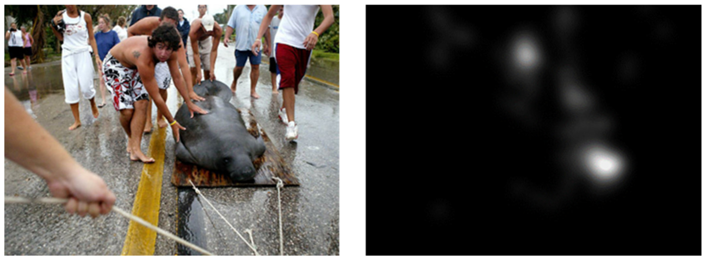
Understand high-level semantics: The deep saliency models are good at extracting common features, such as humans and textures, among others. The saliency predictor can also be used to handle these features. However, as shown in Figure 5, the most interesting or significant parts of an image are not necessarily all of these features. Human visual models often entail a reasoning process based on sensory stimuli. To establish the reason behind the relative importance of image regions on the saliency model, researchers can use higher-level features, such as emotions, gaze direction, and body posture. Moreover, aiming to approach the human-level saliency prediction, researchers need to carry out cognitive attention research to help overcome the aforementioned limitations. A few useful explorations have been offered. For example, Zhao [98] showed through his experimental results that emotion has a priority effect. Nonetheless, the existing saliency model still cannot fully explain the high-level semantics in the scene. The concept of “semantic gap” and the process of determining the relative importance of objects still cannot be resolved; moreover, whether the saliency in natural scenes is guided by objects or low-level features is a matter of debate [124]. The research on the saliency prediction task is closely related to cognitive disciplines, and its findings can help to improve the subsequent various visual research.

With the great success of the deep model in saliency prediction, new developments in deep learning have also provided the possibility for new applications and tasks of saliency models. For example, Aksoy et al. [16] proposed a novel attention-based model for making braking decisions and other driving decisions like steering and acceleration. Jia et al. [19] proposed a multimodal salient wave detection network for sleep staging called SalientSleepNet, which translated the time series classification problem into a saliency detection problem and applies it to sleep stage classification. Wei et al. [125] used a saliency model to pursue their research on autism spectrum disorder (ASD). They found that children with ASD, particularly autism, were informed by special objects and less on social objects (e.g., face), and the application of the verification model of obviousness is helpful in monitoring and evaluating their condition. O’Shea et al. [126] proposed a model for detecting seizure events from raw electroencephalogram (EEG) signals with less dependency on the availability of precise clinical labels. This work opens new avenues for the application of deep learning to neonatal EEG. Theism et al. [127] used a fully connected network and Fisher pruning to increase the saliency calculation speed by 10 times as a means of providing ideas for applications with high real-time requirements. Fan et al. [128] proposed a model to detect shared attention in videos to infer shared attention in third-person social scene videos, which were significant for studying human social interactions. They proposed a new video dataset VACATION [129] and a spatial-temporal graph reasoning model to explicitly represent the diverse gaze interactions in the social scenes and to infer atomic-level gaze communication by message passing.

9. Conclusions

The development of visual saliency prediction tasks has produced numerous methods, and all of them have played an important role in various research directions. Deep networks can automatically capture features and effectively combine feature extraction and saliency prediction. Furthermore, performance can be significantly improved with respect to the classic model that uses handcrafted features. However, the features extracted by the deep saliency model may not fully represent the salient objects and regions in an image, especially in complex scenes that contain advanced information, such as emotion, text, or symbolic information. In view of further improving the performance of the model, the reasoning process of HVS must be imitated to realize the discrimination of relatively important areas in the scene.

In this review, we have summarized the literature about saliency prediction, including the early psychological and physiological mechanisms, the classic models affected by this task, the introduction of visual saliency models based on deep learning, and the data comparisons and summaries in the static and dynamic fields. The reasons for the superiority and the limitations of the saliency model are also analyzed, and the ways of improvement and possible development directions are identified. Although the visual saliency model based on deep learning has made great progress, there is still room for exploration in the aspects of visualization and multi-modality and the understanding of high-level semantics, especially the research on attention mechanisms and the application related to cognitive science.

References

- Itti, L.; Koch, C. Computational modelling of visual attention. Nat. Rev. Neurosci. 2001, 2, 194–203. [Google Scholar] [CrossRef] [PubMed] [Green Version]
- Sziklai, G.C. Some studies in the speed of visual perception. IRE Trans. Inf. Theory 1956, 76, 125–128. [Google Scholar] [CrossRef]
- Koch, K.; Mclean, J.; Segev, R.; Freed, M.A.; Michael, I.I.; Balasubramanian, V.; Sterling, P. How Much the Eye Tells the Brain. Curr. Biol. 2006, 16, 1428–1434. [Google Scholar] [CrossRef] [PubMed] [Green Version]
- Itti, L. A model of saliency-based visual attention for rapid scene analysis. IEEE Trans. 1998, 20, 1254–1259. [Google Scholar] [CrossRef] [Green Version]
- Han, J.; Ngan, K.N.; Li, M.; Zhang, H.J. Unsupervised extraction of visual attention objects in color images. IEEE Trans. Circuits Syst. Video Technol. 2005, 16, 141–145. [Google Scholar] [CrossRef]
- Jung, C.; Kim, C. A Unified Spectral-Domain Approach for Saliency Detection and Its Application to Automatic Object Segmentation. IEEE Trans. Image Process. A Publ. IEEE Signal Process. Soc. 2012, 21, 1272–1283. [Google Scholar] [CrossRef]
- Siagian, C.; Itti, L. Biologically Inspired Mobile Robot Vision Localization. IEEE Trans. Robot. 2009, 25, 861–873. [Google Scholar] [CrossRef] [Green Version]
- Koch, C.; Ullman, S. Shifts in Selective Visual Attention: Towards the Underlying Neural Circuitry. Hum. Neurobiol. 1987, 4, 219–227. [Google Scholar]
- Tong, Y.; Cheikh, F.A.; Guraya, F.; Konik, H.; Trémeau, A. A Spatiotemporal Saliency Model for Video Surveillance. Cogn. Comput. 2011, 3, 241–263. [Google Scholar]
- Itti, L. Automatic foveation for video compression using a neurobiological model of visual attention. IEEE Trans. Image Process. 2004, 13, 1304–1318. [Google Scholar] [CrossRef] [Green Version]
- Monga, V.; Evans, B.L. Perceptual Image Hashing Via Feature Points: Performance Evaluation and Tradeoffs. IEEE Trans. Image Process. A Publ. IEEE Signal Process. Soc. 2006, 15, 3452–3465. [Google Scholar] [CrossRef]
- Wang, W.; Shen, J.; Dong, X.; Borji, A.; Yang, R. Inferring Salient Objects from Human Fixations. Inferring salient objects from human fixations. IEEE Trans. Pattern Anal. Mach. Intell. 2019, 42, 1913–1927. [Google Scholar] [CrossRef]
- Wang, W.; Shen, J.; Lu, X.; Hoi, S.C.H.; Ling, H. Paying Attention to Video Object Pattern Understanding. IEEE Trans. Pattern Anal. Mach. Intell. 2020, 43, 2413–2428. [Google Scholar] [CrossRef]
- Wang, W.; Shen, J.; Ling, H. A Deep Network Solution for Attention and Aesthetics Aware Photo Cropping. IEEE Trans. Pattern Anal. Mach. Intell. 2018, 41, 1531–1544. [Google Scholar] [CrossRef]
- Wang, K.; Ma, S.; Chen, J.; Lu, J. Salient Bundle Adjustment for Visual SLAM. IEEE Trans. Instrum. Meas. 2020, 70, 1–9. [Google Scholar] [CrossRef]
- Aksoy, E.; Yazc, A.; Kasap, M. See, Attend and Brake: An Attention-based Saliency Map Prediction Model for End-to-End Driving. arXiv 2020, arXiv:2002.11020. [Google Scholar]
- Lu, J.; Yang, J.; Batra, D.; Parikh, D. Hierarchical co-attention for visual question answering. Adv. Neural Inf. Process. Syst. 2016, 29, 289–297. [Google Scholar]
- Wang, S.; Jiang, M.; Duchesne, X.; Laugeson, E.; Kennedy, D.; Adolphs, R.; Zhao, Q. Atypical Visual Saliency in Autism Spectrum Disorder Quantified through Model-Based Eye Tracking. Neuron 2015, 88, 604–616. [Google Scholar] [CrossRef] [Green Version]
- Jia, Z.; Lin, Y.; Wang, J.; Wang, X.; Xie, P.; Zhang, Y. SalientSleepNet: Multimodal Salient Wave Detection Network for Sleep Staging. arXiv 2021, arXiv:2105.13864. [Google Scholar]
- Wang, W.; Lai, Q.; Fu, H.; Shen, J.; Yang, R. Salient Object Detection in the Deep Learning Era: An In-depth Survey. IEEE Trans. Pattern Anal. Mach. Intell. 2021, 1448–1457. [Google Scholar] [CrossRef]
- Wang, W.; Shen, J.; Cheng, M.M.; Shao, L. An Iterative and Cooperative Top-Down and Bottom-Up Inference Network for Salient Object Detection. In Proceedings of the CVPR19, Long Beach, CA, USA, 16–20 June 2019. [Google Scholar]
- Wang, W.; Zhao, S.; Shen, J.; Hoi, S.; Borji, A. Salient Object Detection With Pyramid Attention and Salient Edges. In Proceedings of the CVPR19, Long Beach, CA, USA, 16–20 June 2019. [Google Scholar]
- Zhang, J.; Dai, Y.; Yu, X.; Harandi, M.; Barnes, N.; Hartley, R. Uncertainty-Aware Deep Calibrated Salient Object Detection. arXiv 2020, arXiv:2012.06020. [Google Scholar]
- Zhang, P.; Liu, W.; Zeng, Y.; Lei, Y.; Lu, H. Looking for the Detail and Context Devils: High-Resolution Salient Object Detection. IEEE Trans. Image Process. 2021, 30, 3204–3216. [Google Scholar] [CrossRef]
- Treisman, A.M.; Gelade, G. A feature-integration theory of attention. Cogn. Psychol. 1980, 12, 97–136. [Google Scholar] [CrossRef]
- Treisman, A. Feature binding, attention and object perception. Philos. Trans. R. Soc. B Biol. Sci. 1998, 353, 1295–1306. [Google Scholar] [CrossRef] [Green Version]
- Wolfe, J.M. Guided Search 2.0 A revised model of visual search. Psychon. Bull. Rev. 1994, 1, 202–238. [Google Scholar] [CrossRef] [Green Version]
- Harel, J.; Koch, C.; Perona, P. Graph-Based Visual Saliency. In Proceedings of the IEEE Conference on Advances in Neural Information Processing Systems, Vancouver, BC, Canada, 4–9 December 2006. [Google Scholar]
- Ma, Y.F. Contrast-based image attention analysis by using fuzzy growing. In Proceedings of the 11th Annual ACM International Conference on Multimedia, Berkeley, CA, USA, 2–8 November 2003. [Google Scholar]
- Liu, T.; Yuan, Z.; Sun, J.; Wang, J.; Zheng, N.; Tang, X.; Shum, H.-Y. Learning to detect a salient object. IEEE Trans. Pattern Anal. Mach. Intell. 2010, 33, 353–367. [Google Scholar]
- Borji, A.; Itti, L. Exploiting local and global patch rarities for saliency detection. In Proceedings of the Conference on Computer Vision and Pattern Recognition (CVPR), Providence, RI, USA, 16–21 June 2012. [Google Scholar]
- Zhang, J.; Sclaroff, S. Saliency Detection: A Boolean Map Approach. In Proceedings of the 2013 IEEE International Conference on Computer Vision, Sydney, Australia, 1–8 December 2013. [Google Scholar]
- Zhai, Y.; Shah, M. Visual attention detection in video sequences using spatiotemporal cues. In Proceedings of the 14th ACM International Conference on Multimedia, Santa Barbara, CA, USA, 23–27 October 2006. [Google Scholar]
- Wei, Y.; Jie, F.; Tao, L.; Jian, S. Salient object detection by composition. In Proceedings of the IEEE International Conference on Computer Vision, ICCV 2011, Barcelona, Spain, 6–13 November 2011. [Google Scholar]
- Margolin, R.; Tal, A.; Zelnik-Manor, L. What Makes a Patch Distinct? In Proceedings of the IEEE Conference on Computer Vision and Pattern Recognition (CVPR). Portland, OR, USA, 23–28 June 2013. [Google Scholar]
- Achanta, R.; Hemami, S.; Estrada, F.; Su¨Sstrunk, S. Frequency-tuned salient region detection. In Proceedings of the 2009 IEEE Conference on Computer Vision and Pattern Recognition, Miami, FL, USA, 20–25 June 2009; pp. 1597–1604. [Google Scholar]
- Cheng, M.M.; Zhang, G.X.; Mitra, N.J.; Huang, X.; Hu, S.M. Global Contrast Based Salient Region Detection. In Proceedings of the Computer Vision and Pattern Recognition, Colorado Springs, CO, USA, 20–25 June 2011. [Google Scholar]
- Zhi, L.; Zhang, X.; Luo, S.; Meur, O.L. Superpixel-Based Spatiotemporal Saliency Detection. IEEE Trans. Circuits Syst. Video Technol. 2014, 24, 1522–1540. [Google Scholar]
- Ren, Z.; Hu, Y.; Chia, L.T.; Rajan, D. Improved saliency detection based on superpixel clustering and saliency propagation. In Proceedings of the Acm International Conference on Multimedia, Firenze, Italy, 25–29 October 2010. [Google Scholar]
- Huang, G.; Pun, C.M.; Lin, C. Unsupervised video co-segmentation based on superpixel co-saliency and region merging. Multimed. Tools Appl. 2016, 76, 12941–12964. [Google Scholar] [CrossRef]
- Bruce, N.D.B.; Tsotsos, J.K. Saliency Based on Information Maximization. In Proceedings of the Advances in Neural Information Processing Systems 18, Vancouver, BC, Canada, 5–8 December 2005. [Google Scholar]
- Hou, X. Dynamic visual attention: Searching for coding length increments. In Proceedings of the Advances in Neural Information Processing Systems (NIPS, 2008), Vancouver, BC, Canada, 8–10 December 2008; pp. 681–688. [Google Scholar]
- Mancas, M.; Mancas-Thillou, C.; Gosselin, B.; Macq, B.M. A Rarity-Based Visual Attention Map–Application to Texture Description. In Proceedings of the International Conference on Image Processing, ICIP 2006, Atlanta, GA, USA, 8–11 October 2006. [Google Scholar]
- Seo, H.J.; Milanfar, P. Nonparametric bottom-up saliency detection by self-resemblance. In Proceedings of the 2009 IEEE Computer Society Conference on Computer Vision and Pattern Recognition Workshops, Miami, FL, USA, 20–25 June 2009; pp. 45–52. [Google Scholar]
- Rosenholtz, R.; Nagy, A.L.; Bell, N.R. The effect of background color on asymmetries in color search. J. Vis. 2004, 4, 224–240. [Google Scholar] [CrossRef] [PubMed]
- Hou, X.; Zhang, L. Saliency Detection: A Spectral Residual Approach. In Proceedings of the IEEE Conference on Computer Vision & Pattern Recognition, Minneapolis, MN, USA, 17–22 June 2007. [Google Scholar]
- Guo, C.; Qi, M.; Zhang, L. Spatio-temporal Saliency detection using phase spectrum of quaternion fourier transform. In Proceedings of the IEEE Conference on Computer Vision & Pattern Recognition, Anchorage, AK, USA, 23–28 June 2008. [Google Scholar]
- Holtzman-Gazit, M.; Zelnik-Manor, L.; Yavneh, I. Salient Edges: A Multi Scale Approach. In Proceedings of the 11th European Conference on Computer Vision, Crete, Greece, 5–11 September 2010; p. 4310. [Google Scholar]
- Sclaroff, J. Exploiting Surroundedness for Saliency Detection: A Boolean Map Approach. IEEE Comput. Soc. 2016, 38, 889–902. [Google Scholar]
- Borji, A.; Itti, L. State-of-the-Art in Visual Attention Modeling. IEEE Trans. Pattern Anal. Mach. Intell. 2013, 35, 185–207. [Google Scholar] [CrossRef]
- Oliva, A.; Torralba, A.; Castelhano, M.S.; Henderson, J.M. Top-down control of visual attention in object detection. In Proceedings of the International Conference on Image Processing, Barcelona, Spain, 14–18 September 2003; pp. I 253–256. [Google Scholar]
- Ehinger, K.A.; Hidalgo-Sotelo, B.; Torralba, A.; Oliva, A. Modelling search for people in 900 scenes: A combined source model of eye guidance. Vis. Cogn. 2009, 17, 945–978. [Google Scholar] [CrossRef] [Green Version]
- Xie, Y.; Lu, H.; Yang, M.H. Bayesian Saliency via Low and Mid Level Cues. IEEE Trans. Image Process. A Publ. IEEE Signal Process. Soc. 2013, 22, 1689–1698. [Google Scholar]
- Zhang, L.; Tong, M.; Marks, H.; Tim, K.; Shan, H.; Cottrell, G. SUN: A Bayesian framework for saliency using natural statistics. J. Vis. 2008, 8, 32. [Google Scholar] [CrossRef] [Green Version]
- Gao, D.; Vasconcelos, N. Discriminant Saliency for Visual Recognition from Cluttered Scenes. In Proceedings of the Advances in Neural Information Processing Systems 17 [Neural Information Processing Systems, NIPS 2004], Vancouver, BC, Canada, 12–18 December 2004. [Google Scholar]
- Gao, D.; Vasconcelos, N. Decision-Theoretic Saliency: Computational Principles, Biological Plausibility, and Implications for Neurophysiology and Psychophysics. Neural Comput. 2014, 21, 239–271. [Google Scholar] [CrossRef]
- Kim, H.; Kim, Y.; Sim, J.Y.; Kim, C.S. Spatiotemporal saliency in dynamic scenes. IEEE Trans. Pattern Anal. Mach. Intell. 2015, 32, 171–177. [Google Scholar]
- Gu, E.; Wang, J.; Badler, N.I. Generating Sequence of Eye Fixations Using Decision-theoretic Attention Model. In Proceedings of the IEEE Computer Society Conference on Computer Vision & Pattern Recognition, San Diego, CA, USA, 20–26 June 2005. [Google Scholar]
- Kienzle, W.; Franz, M.O.; Scholkopf, B.; Wichmann, F.A. Center-surround patterns emerge as optimal predictors for human saccade targets. J. Vis. 2009, 9, 1–15. [Google Scholar] [CrossRef] [Green Version]
- Peters, R.J.; Itti, L. Beyond bottom-up: Incorporating task-dependent influences into a computational model of spatial attention. In Proceedings of the IEEE Conference on Computer Vision & Pattern Recognition, Minneapolis, MN, USA, 17–22 June 2007. [Google Scholar]
- Judd, T.; Ehinger, K.; Durand, F.; Torralba, A. Learning to Predict Where Humans Look. In Proceedings of the IEEE 12th International Conference on Computer Vision, ICCV 2009, Kyoto, Japan, 27 September–4 October 2009. [Google Scholar]
- Vig, E.; Dorr, M.; Cox, D. Large-Scale Optimization of Hierarchical Features for Saliency Prediction in Natural Images. In Proceedings of the 2014 IEEE Conference on Computer Vision and Pattern Recognition (CVPR), Columbus, OH, USA, 23–28 June 2014. [Google Scholar]
- Kümmerer, M.; Theis, L.; Bethge, M. Deep Gaze I: Boosting Saliency Prediction with Feature Maps Trained on ImageNet. arXiv 2014, arXiv:1411.1045. [Google Scholar]
- Krizhevsky, A.; Sutskever, I.; Hinton, G.E. Imagenet classification with deep convolutional neural networks. Adv. Neural Inf. Process. Syst. 2012, 25, 1097–1105. [Google Scholar] [CrossRef]
- Jia, D.; Wei, D.; Socher, R.; Li, L.J.; Kai, L.; Li, F.F. ImageNet: A large-scale hierarchical image database. In Proceedings of the 2009 IEEE Conference on Computer Vision and Pattern Recognition, Miami, FL, USA, 20–25 June 2009; pp. 248–255. [Google Scholar]
- Kruthiventi, S.; Ayush, K.; Babu, R.V. DeepFix: A Fully Convolutional Neural Network for Predicting Human Eye Fixations. IEEE Trans. Image Process. 2017, 26, 4446–4456. [Google Scholar] [CrossRef] [Green Version]
- Simonyan, K.; Zisserman, A. Very Deep Convolutional Networks for Large-Scale Image Recognition. arXiv 2014, arXiv:1409.1556. [Google Scholar]
- Kümmerer, M.; Wallis, T.; Bethge, M. DeepGaze II: Reading fixations from deep features trained on object recognition. arXiv 2016, arXiv:1610.01563. [Google Scholar]
- Ming, J.; Huang, S.; Duan, J.; Qi, Z. SALICON: Saliency in Context. In Proceedings of the Computer Vision & Pattern Recognition, Boston, MA, USA, 7–12 June 2015. [Google Scholar]
- Azam, S.; Gilani, S.O.; Jeon, M.; Yousaf, R.; Kim, J.-B. A Benchmark of Computational Models of Saliency to Predict Human Fixations in Videos. In VISIGRAPP (4: VISAPP); SCITEPRESS—Science and Technology Publications, Lda.: Setúbal, Portugal, 2016; pp. 134–142. [Google Scholar]
- Pan, J.; Mcguinness, K.; Sayrol, E.; O’Connor, N.; Giro-I-Nieto, X. Shallow and Deep Convolutional Networks for Saliency Prediction. arXiv 2016, arXiv:1603.00845. [Google Scholar]
- Jetley, S.; Murray, N.; Vig, E. End-to-end saliency mapping via probability distribution prediction. In Proceedings of the IEEE Conference on Computer Vision and Pattern Recognition, Las Vegas, NV, USA, 27–30 June 2016; pp. 5753–5761. [Google Scholar]
- Liu, N.; Han, J. A Deep Spatial Contextual Long-Term Recurrent Convolutional Network for Saliency Detection. IEEE Trans. Image Process. A Publ. IEEE Signal Process. Soc. 2018, 27, 3264–3274. [Google Scholar] [CrossRef] [Green Version]
- Cornia, M.; Baraldi, L.; Serra, G.; Cucchiara, R. A Deep Multi-Level Network for Saliency Prediction. In Proceedings of the International Conference on Pattern Recognition, Cancun, Mexico, 4–8 December 2016. [Google Scholar]
- Marcella, C.; Lorenzo, B.; Giuseppe, S.; Rita, C. Predicting Human Eye Fixations via an LSTM-based Saliency Attentive Model. IEEE Trans. Image Process. 2016, 27, 5142–5154. [Google Scholar]
- Pan, J.; Canton, C.; Mcguinness, K.; O’Connor, N.E.; Giro-I-Nieto, X. SalGAN: Visual Saliency Prediction with Generative Adversarial Networks. arXiv 2017, arXiv:1701.01081. [Google Scholar]
- Jia, S.; Bruce, N.D.B. EML-NET:An Expandable Multi-Layer NETwork for Saliency Prediction. arXiv 2018, arXiv:1805.01047. [Google Scholar]
- Wenguan; Wang; Jianbing; Shen. Deep Visual Attention Prediction. IEEE Trans. Image Process. 2017, 27, 2368–2378. [Google Scholar]
- Gorji, S.; Clark, J.J. Attentional Push: A Deep Convolutional Network for Augmenting Image Salience with Shared Attention Modeling in Social Scenes. In Proceedings of the 2017 IEEE Conference on Computer Vision and Pattern Recognition (CVPR), Honolulu, HI, USA, 21–26 July 2017. [Google Scholar]
- Dodge, S.; Karam, L. Visual Saliency Prediction Using a Mixture of Deep Neural Networks. IEEE Trans. Image Process. 2017, 27, 4080–4090. [Google Scholar] [CrossRef]
- Mahdi, A.; Qin, J.; Crosby, G. DeepFeat: A bottom-up and top-down saliency model based on deep features of convolutional neural networks. IEEE Trans. Cogn. Dev. Syst. 2019, 12, 54–63. [Google Scholar] [CrossRef]
- Aka, B.; Msa, B.; Kd, C.; Rgab, D. Contextual encoder–decoder network for visual saliency prediction. Neural Netw. 2020, 129, 261–270. [Google Scholar]
- Gao, D.; Mahadevan, V.; Vasconcelos, N. The discriminant center-surround hypothesis for bottom-up saliency. In Proceedings of the Advances in Neural Information Processing Systems 20, Proceedings of the Twenty-First Annual Conference on Neural Information Processing Systems, Vancouver, BC, Canada, 3–6 December 2007. [Google Scholar]
- Seo, H.J.; Milanfar, P. Using local regression kernels for statistical object detection. In Proceedings of the IEEE International Conference on Image Processing, San Diego, CA, USA, 12–15 October 2008. [Google Scholar]
- Bak, C.; Kocak, A.; Erdem, E.; Erdem, A. Spatio-temporal saliency networks for dynamic saliency prediction. IEEE Trans. Multimed. 2017, 20, 1688–1698. [Google Scholar] [CrossRef] [Green Version]
- Chaabouni, S.; Benois-Pineau, J.; Amar, C.B. Transfer learning with deep networks for saliency prediction in natural vide. In Proceedings of the 2016 IEEE International Conference on Image Processing (ICIP), Phoenix, AZ, USA, 25–28 September 2016. [Google Scholar]
- Leifman, G.; Rudoy, D.; Swedish, T.; Bayro-Corrochano, E.; Raskar, R. Learning Gaze Transitions from Depth to Improve Video Saliency Estimation. In Proceedings of the 2017 IEEE International Conference on Computer Vision (ICCV), Venice, Italy, 22–29 October 2017. [Google Scholar]
- Lai, Q.; Wang, W.; Sun, H.; Shen, J. Video Saliency Prediction using Spatiotemporal Residual Attentive Networks. IEEE Trans. Image Process. 2019, 29, 1113–1126. [Google Scholar] [CrossRef] [PubMed]
- Bazzani, L.; Larochelle, H.; Torresani, L. Recurrent Mixture Density Network for Spatiotemporal Visual Attention. arXiv 2016, arXiv:1603.08199. [Google Scholar]
- Jiang, L.; Xu, M.; Wang, Z. Predicting Video Saliency with Object-to-Motion CNN and Two-layer Convolutional LSTM. arXiv 2017, arXiv:1709.06316. [Google Scholar]
- Gorji, S.; Clark, J.J. Going from Image to Video Saliency: Augmenting Image Salience with Dynamic Attentional Push. In Proceedings of the 2018 IEEE/CVF Conference on Computer Vision and Pattern Recognition (CVPR), Salt Lake City, UT, USA, 18–23 June 2018. [Google Scholar]
- Wang, W.; Shen, J.; Fang, G.; Cheng, M.M.; Borji, A. Revisiting Video Saliency: A Large-Scale Benchmark and a New Model. In Proceedings of the 2018 IEEE/CVF Conference on Computer Vision and Pattern Recognition (CVPR), Salt Lake City, UT, USA, 18–23 June 2018. [Google Scholar]
- Zhang, K. A Spatial-Temporal Recurrent Neural Network for Video Saliency Prediction. IEEE Trans. Image Process. 2020, 30, 572–587. [Google Scholar] [CrossRef]
- Xu, M.; Yang, L.; Tao, X.; Duan, Y.; Wang, Z. Saliency Prediction on Omnidirectional Image With Generative Adversarial Imitation Learning. IEEE Trans. Image Process. 2021, 30, 2087–2102. [Google Scholar] [CrossRef]
- Yang, C.; Zhang, L.; Lu, H.; Ruan, X.; Yang, M.H. Saliency Detection via Graph-Based Manifold Ranking. In Proceedings of the Computer Vision & Pattern Recognition, Portland, OR, USA, 23–28 June 2013. [Google Scholar]
- Borji, A.; Itti, L. CAT2000: A Large Scale Fixation Dataset for Boosting Saliency Research. arXiv 2015, arXiv:1505.03581. [Google Scholar]
- Borji, A.; Tavakoli, H.R.; Sihite, D.N.; Itti, L. Analysis of Scores, Datasets, and Models in Visual Saliency Prediction. In Proceedings of the IEEE International Conference on Computer Vision, Columbus, OH, USA, 23–28 June 2014. [Google Scholar]
- Fan, S.; Shen, Z.; Ming, J.; Koenig, B.L.; Qi, Z. Emotional Attention: A Study of Image Sentiment and Visual Attention. In Proceedings of the 2018 IEEE/CVF Conference on Computer Vision and Pattern Recognition, Salt Lake City, UT, USA, 18–23 June 2018. [Google Scholar]
- Mital, P.K.; Smith, T.J.; Hill, R.L.; Henderson, J.M. Clustering of Gaze During Dynamic Scene Viewing is Predicted by Motion. Cogn. Comput. 2011, 3, 5–24. [Google Scholar] [CrossRef]
- Mathe, S.; Sminchisescu, C. Actions in the Eye: Dynamic Gaze Datasets and Learnt Saliency Models for Visual Recognition. IEEE Trans. Pattern Anal. Mach. Intell. 2015, 37, 1408–1424. [Google Scholar] [CrossRef] [Green Version]
- Jiang, L.; Xu, M.; Liu, T.; Qiao, M.; Wang, Z. Deepvs: A deep learning based video saliency prediction approach. In Proceedings of the European Conference on Computer Vision (ECCV), Munich, Germany, 8–14 September 2018; pp. 602–617. [Google Scholar]
- Judd, T.; Durand, F.; Torralba, A. A Benchmark of Computational Models of Saliency to Predict Human Fixations; Technical Report MIT-CSAIL-TR-2012-001; MIT Libraries: Cambridge, MA, USA, 2012. [Google Scholar]
- Borji, A.; Sihite, D.N.; Itti, L. Quantitative Analysis of Human-Model Agreement in Visual Saliency Modeling: A Comparative Study. IEEE Trans. Image Process. 2013, 22, 55–69. [Google Scholar] [CrossRef] [Green Version]
- Peters, R.J.; Iyer, A.; Itti, L.; Koch, C. Components of bottom-up gaze allocation in natural images. Vis. Res. 2005, 45, 2397–2416. [Google Scholar] [CrossRef] [Green Version]
- Rubner, Y.; Tomasi, C.; Guibas, L.J. The Earth Mover’s Distance as a Metric for Image Retrieval. Int. J. Comput. Vis. 2000, 40, 99–121. [Google Scholar] [CrossRef]
- Tavakoli, H.R.; Borji, A.; Laaksonen, J.; Rahtu, E. Exploiting inter-image similarity and ensemble of extreme learners for fixation prediction using deep features. Neurocomputing 2017, 244, 10–18. [Google Scholar] [CrossRef] [Green Version]
- Zanca, D.; Gori, M. Variational Laws of Visual Attention for Dynamic Scenes. In Proceedings of the NIPS 2017, Long Beach, CA, USA, 4–9 December 2017. [Google Scholar]
- Shu, F.; Jia, L.; Tian, Y.; Huang, T.; Chen, X. Learning Discriminative Subspaces on Random Contrasts for Image Saliency Analysis. IEEE Trans. Neural Netw. Learn. Syst. 2017, 28, 1095–1108. [Google Scholar]
- Tavakoli, H.R.; Rahtu, E.; Heikkilä, J. Fast and efficient saliency detection using sparse sampling and kernel density estimation. In Proceedings of the Scandinavian Conference on Image Analysis, Ystad, Sweden, 23–27 May 2011; pp. 666–675. [Google Scholar]
- Aboudib, A.; Gripon, V.; Coppin, G. A model of bottom-up visual attention using cortical magnification. In Proceedings of the IEEE International Conference on Acoustics, South Brisbane, QLD, Australia, 19–24 April 2015. [Google Scholar]
- Goferman, S.; Zelnik-Manor, L.; Tal, A. Context-aware saliency detection. IEEE Trans. Pattern Anal. Mach. Intell. 2011, 34, 1915–1926. [Google Scholar] [CrossRef] [Green Version]
- Garcia-Diaz, A.; Leboran, V.; Fdez-Vidal, X.R.; Pardo, X.M. On the relationship between optical variability, visual saliency, and eye fixations: A computational approach. J. Vis. 2012, 12, 17. [Google Scholar] [CrossRef] [Green Version]
- Lopez-Garcia, F.; Fdez-Vidal, X.R.; Pardo, X.M.; Dosil, R. Scene recognition through visual attention and image features: A comparison between sift and surf approaches. Object Recognit. 2011, 4, 185–200. [Google Scholar]
- Fang, Y.; Wang, Z.; Lin, W. Video Saliency Incorporating Spatiotemporal Cues and Uncertainty Weighting. In Proceedings of the 2013 IEEE International Conference on Multimedia and Expo (ICME), San Jose, CA, USA, 15–19 July 2013. [Google Scholar]
- Rudoy, D.; Dan, B.G.; Shechtman, E.; Zelnik-Manor, L. Learning Video Saliency from Human Gaze Using Candidate Selection. In Proceedings of the 2013 IEEE Conference on Computer Vision and Pattern Recognition, Portland, OR, USA, 23–28 June 2013. [Google Scholar]
- Leboran, V.; Garcia-Diaz, A.; Fdez-Vidal, X.R.; Pardo, X.M. Dynamic whitening saliency. IEEE Trans. Pattern Anal. Mach. Intell. 2016, 39, 893–907. [Google Scholar] [CrossRef]
- Dedieu, J.F.; Gazin, C.; Rigolet, M.; Galibert, F. A Novel Multiresolution Spatiotemporal Saliency Detection Model and Its Applications in Image and Video Compression. Oncogene 1988, 3, 523–529. [Google Scholar]
- Khatoonabadi, S.H.; Vasconcelos, N.; Bajic, I.V.; Shan, N.Y. How many bits does it take for a stimulus to be salient? In Proceedings of the 2015 IEEE Conference on Computer Vision & Pattern Recognition, Boston, MA, USA, 7–12 June 2015.
- Seo, H.J.; Milanfar, P. Static and space-time visual saliency detection by self-resemblance. J. Vis. 2009, 9, 15. [Google Scholar] [CrossRef] [Green Version]
- Bruce, N.D.B.; Wloka, C.; Frosst, N.; Rahman, S.; Tsotsos, J.K. On computational modeling of visual saliency: Examining what’s right, and what’s left. Vis. Res. 2015, 116, 95–112. [Google Scholar] [CrossRef]
- Sun, C.; Shrivastava, A.; Singh, S.; Gupta, A. Revisiting Unreasonable Effectiveness of Data in Deep Learning Era. In Proceedings of the 2017 IEEE International Conference on Computer Vision (ICCV), Venice, Italy, 22–29 October 2017. [Google Scholar]
- Coutrot, A.; Guyader, N. How saliency, faces, and sound influence gaze in dynamic social scenes. J. Vis. 2014, 14, 5. [Google Scholar] [CrossRef]
- Bylinskii, Z.; Alsheikh, S.; Madan, S.; Recasens, A.; Zhong, K.; Pfister, H.; Durand, F.; Oliva, A. Understanding Infographics through Textual and Visual Tag Prediction. arXiv 2017, arXiv:1709.09215. [Google Scholar]
- Stoll, J.; Thrun, M.; Nuthmann, A.; Einhäuser, W. Overt attention in natural scenes: Objects dominate features. Vis. Res. An. Int. J. Vis. Sci. 2015, 107, 36–48. [Google Scholar] [CrossRef] [Green Version]
- Wei, W.; Liu, Z.; Huang, L.; Nebout, A.; Meur, O.L. Saliency Prediction via Multi-Level Features and Deep Supervision for Children with Autism Spectrum Disorder. In Proceedings of the 2019 IEEE International Conference on Multimedia & Expo Workshops (ICMEW), Shanghai, China, 8–12 July 2019. [Google Scholar]
- O’Shea, A.; Lightbody, G.; Boylan, G.; Temko, A. Neonatal seizure detection from raw multi-channel EEG using a fully convolutional architecture. arXiv 2021, arXiv:2105.13854. [Google Scholar] [CrossRef]
- Theis, L.; Korshunova, I.; Tejani, A.; Huszár, F. Faster gaze prediction with dense networks and Fisher pruning. arXiv 2018, arXiv:1801.05787. [Google Scholar]
- Fan, L.; Chen, Y.; Wei, P.; Wang, W.; Zhu, S.C. Inferring Shared Attention in Social Scene Videos. In Proceedings of the IEEE CVPR, Salt Lake City, UT, USA, 18–23 June 2018. [Google Scholar]
- Fan, L.; Wang, W.; Huang, S.; Tang, X.; Zhu, S.C. Understanding Human Gaze Communication by Spatio-Temporal Graph Reasoning. arVix 2019, arXiv:1909.02144. [Google Scholar]