Sliding Balance Control of a Point-Foot Biped Robot Based on a Dual-Objective Convergent Equation

Abstract

The point-foot biped robot is highly adaptable to and can move rapidly on complex, non-structural and non-continuous terrain, as demonstrated in many studies. However, few studies have investigated balance control methods for point-foot sliding on low-friction terrain. This article presents a control framework based on the dual-objective convergence method and whole-body control for the point-foot biped robot to stabilize its posture balance in sliding. In this control framework, a dual-objective convergence equation is used to construct the posture stability criterion and the corresponding equilibrium control task, which are simultaneously converged. Control tasks are then carried out through the whole-body control framework, which adopts an optimization method to calculate the viable joint torque under the physical constraints of dynamics, friction and contact forces. In addition, this article extends the proposed approach to balance control in standing recovery. Finally, the capabilities of the proposed controller are verified in simulations in which a 26.9-kg three-link point-foot biped robot (1) slides over a ${10}^{\circ }$ trapezoidal terrain, (2) slides on terrain with a sinusoidal friction coefficient between 0.05 and 0.25 and (3) stands and recovers from a center-of-mass offset of 0.02 m.

1. Introduction

Biped robots, with a legged structure similar to that of biped creatures, are naturally capable of adapting to a variety of environments [1,2]. Biped robots perform better than wheeled and tracked robots on complex, unstructured and discontinuous ground [3,4,5]. To take full advantage of the characteristics of the bipedal structure and to improve the environmental adaptability of biped robots, control algorithms such as those for walking, running, jumping and balance recovery have been designed and adapted to terrains such as grass [6] and stepping stones [7]. Furthermore, biped robots are expected to be widely used in human habitats owing to their human-like shape and in the wild and high-risk environments owing to their wide terrain adaptability. In these environments, it is possible for robots to encounter terrains with low-friction coefficients, such as smooth ceramic tiles, glass floors and hard ice. For such terrains, many robots use an extra device, such as a pulley, skateboard or wheeled foot, to control sliding [8,9,10], which not only limits the robot’s ability to adapt to a wider range of terrain but also increases the robot’s mass and inertia at the end of the leg and deprives the robot of the fast motion characteristic of the point-foot structure. On these types of terrain, the high dynamic characteristics of the point-foot structure make it difficult for the robot to maintain balance by stepping, but the method of adjusting posture is still effective. Therefore, to expand the adaptive ability of the point-foot biped robot, this article investigates a control method of sliding and standing posture balance on ground with a low-friction coefficient.

In recent years, many control methods have been applied to the balance control of biped robots. The key to balance control is to establish the control objective indicating the balance state of the robot. In bipedal control, the center of pressure (CoP) represents the action point of the contact force on the sole of the robot, which is an efficient control objective reflecting the plantar balance [11,12,13,14,15,16]. Macchhietto et al. [14] introduced generalized momentum to design the CoP for standing balance. Similarly, Lee and Goswami [15] defined balance control objectives more intuitively in terms of linear and angular momenta to directly determine the CoP with the ground reaction force and realize balance control on non-level and non-stationary ground. Momentum plays an important role in postural balance, and the centroidal moment point (CMP) has thus been proposed and used to describe the variation in angular momentum [17,18,19,20]. Goswami et al. [17] referred to the CMP as the ZRAM (zero rate of change of angular momentum) point and presented three strategies (i.e., enlarging the support polygon, moving the center of mass (CoM), and changing the direction of the ground reaction force ) to recapture balance. Mayr et al. [19] introduced an excellent CoM–CMP regulator for reference CMP design with linear and angular momentum priority and used the regulator to construct a balance controller for the standing and walking on a humanoid robot. A comparison of these two methods (of Goswami et al. and Mayr et al.) shows that the CMP can be set outside the supporting polygon to expand the stable region of the robot. Shafiee-Ashtiani et al. [20] applied a capture point to evaluate the balance recovery capability and presented a push recovery controller based on a feedback controller by combining the CMP method and ankle strategy to compensate for the error at the CP. The above methods have been shown to work well in postural control and recovery. However, the CoP and CMP have mainly been aimed at the area of contact between the ground and the sole of a foot, and they are difficult to apply to the point-foot of a robot, which is in point contact with the ground. Therefore, a method of keeping the point-foot posture balance by constantly adjusting the foothold has been proposed [21,22]. Nevertheless, adjusting the foothold on ground with a low-friction coefficient is likely to cause the robot to slip and lose its balance. Peng et al. [23] took the angular momentum and its derivative as the equilibrium point and proposed the loss balance degree (LBD) as a stability criterion with which to evaluate the degree to which a biped robot deviates from the equilibrium point. However, they did not apply the method to a specific robot model. Inspired by the revelation of the motion principle of the flywheel inverted-pendulum model using the CMP, in the present study, we combine the flywheel inverted-pendulum model with the Coulomb friction model to reconstruct a sliding model of the robot into a dual-objective convergent form including the posture stability criterion and the equilibrium control target, which not only is suitable for the sliding process but also can be extended to the case of standing balance.

In adjusting the balance of the whole body, most of the joints of the robot are expected to be controlled while maintaining sliding balance. Control methods for sliding biped robots with fewer degrees of freedom (DoFs), such as the wheeled inverted-pendulum robot, have been developed over a period of decades. Many traditional controllers, such as the state-space controller [24], sliding-mode controller [25], and fuzzy controller [26], have been extensively used to control wheeled inverted-pendulum systems. Although these control methods perform well, they are difficult to adapt to more complex bipedal structures. Jeong and Takahashi [27] adopted the linear quadratic regulator (LQR) method to linearize the control model of the robot and realized stable mobile motions for the i-Pentar robot, which comprises a body with a waist and an arm. To use the LQR method, the robot’s model needs to be linearized, which reduces the stability region in the state-space. Meanwhile, it is difficult to use this method to solve control problems under the constraints of friction, contact forces and joint acceleration. Khatib [28] first used inverse dynamics to convert the task space problem to the joint space problem. Adopting the inverse dynamics control method, multi-task motion control can be nonlinearly mapped to joint motion control. Hutter et al. [29] treated the inverse dynamics problem as a quadratic programming (QP) problem and provided an optimization method to solve inverse dynamics problems with constraints. Zafar et al. [30] applied QP whole-body dynamics control to the wheeled humanoid robot with an arm and realized low-level centroid tracking control under the constraint of the joint torque. Klemm et al. [31] extended the wheeled-foot sliding equilibrium capability under non-minimum phase dynamics by considering LQR control as a constraint condition of the QP problem. However, whole-body control is mainly applied to the active movement of a robot with feet and rarely applied to the passive sliding of the point-foot robot. Nevertheless, the control objects of the above algorithms have end-effector devices that can control their speed or angle with the ground, and it is thus difficult to fit with the Coulomb friction characteristics of the ground in point-foot sliding. In this article, we establish the constraint conditions, relaxation factors and cost function for the point-foot robot conforming to sliding conditions using the QP-based whole-body control method.

This article proposes a control framework based on whole-body dynamics control and dual-objective convergence for point-foot bipedal balance control, including sliding and standing balance recoveries, on low-friction terrain. In the control framework, the posture balance controller is a trajectory task generator that includes an equilibrium target generator, torso recovery equilibrium offset generator, and knee trajectory generator, while the whole-body controller is a trajectory-task-to-torque converter that adopts proportional–derivative (PD) control, physical constraints, and the optimization of whole-body dynamics (as shown in Figure 1). First, the robot model based on floating-base coordinates and its corresponding flywheel inverted-pendulum model are analyzed to establish the posture stability criterion and equilibrium control variable, and we use the dual-objective relation between the equilibrium variable and the posture stability criterion to generate the trajectory of the equilibrium target. Second, we build a torso recovery control strategy to generate the equilibrium offset and adjust the posture of the torso. In addition, the posture balance controller generates the knee trajectory. Third, all the trajectory tasks are transformed into corresponding acceleration tasks by a PD controller, and a QP optimizer is applied to map the acceleration tasks to the joint torques under the constraints of dynamics, friction and contact forces. Finally, to verify the proposed method, we set up a multibody physical simulation environment, including sliding balance on uneven terrain, sliding balance on terrain with a variable friction coefficient and standing recovery on terrain with a low-friction coefficient.

The main contributions of this study are (1) the introduction of a dual-objective convergent control method to realize the sliding and standing balance control of an underactuated point-foot bipedal structure, (2) the adoption of a torso recovery strategy based on coefficient regulation and torso state feedback control to adjust the torso posture while maintaining the stability of the whole body, and (3) the adoption of a QP-based whole-body control framework to realize efficient task tracking under physical constraints.

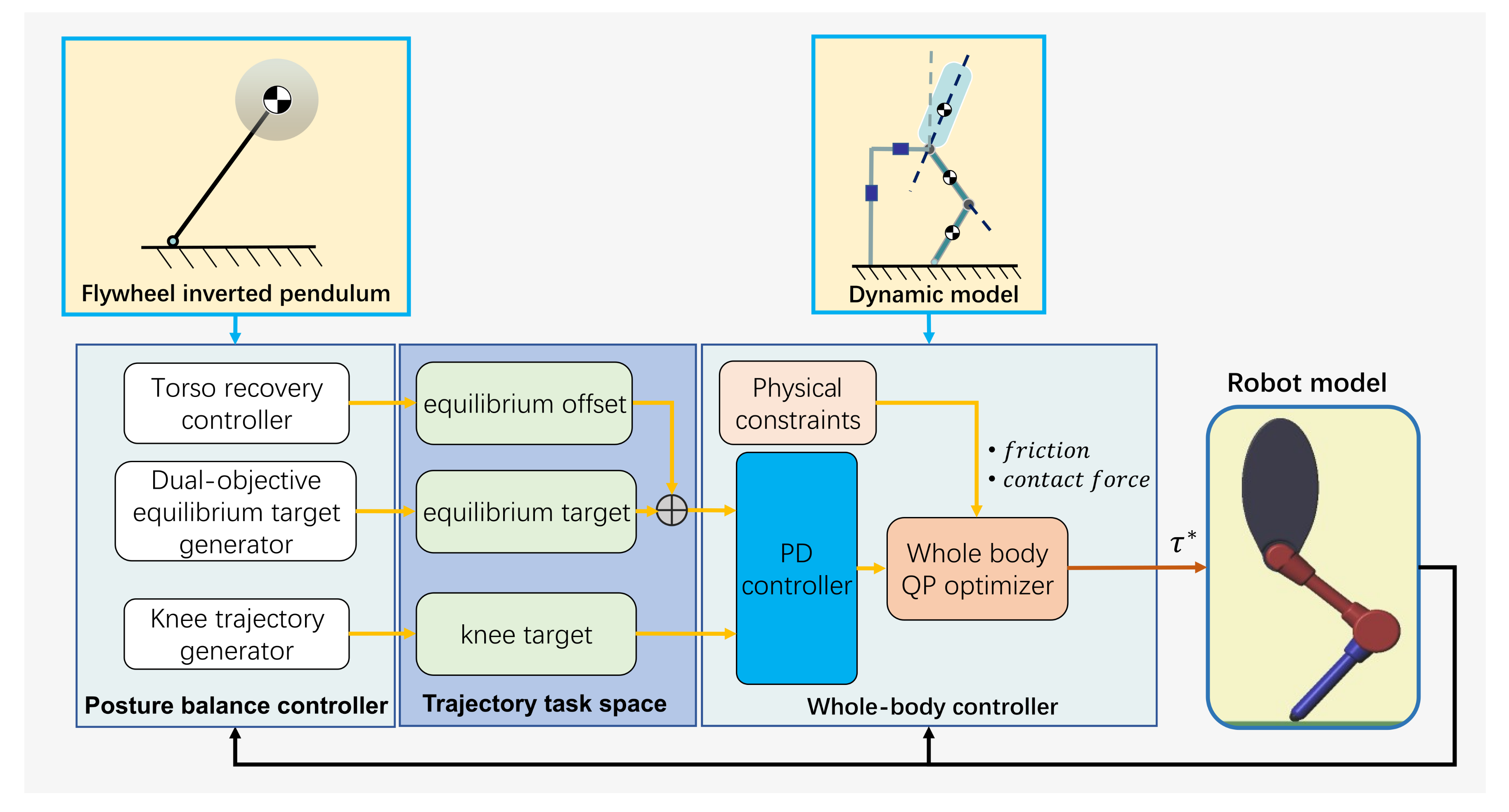
2. Dual-Objective Convergence Equation for the Biped Robot

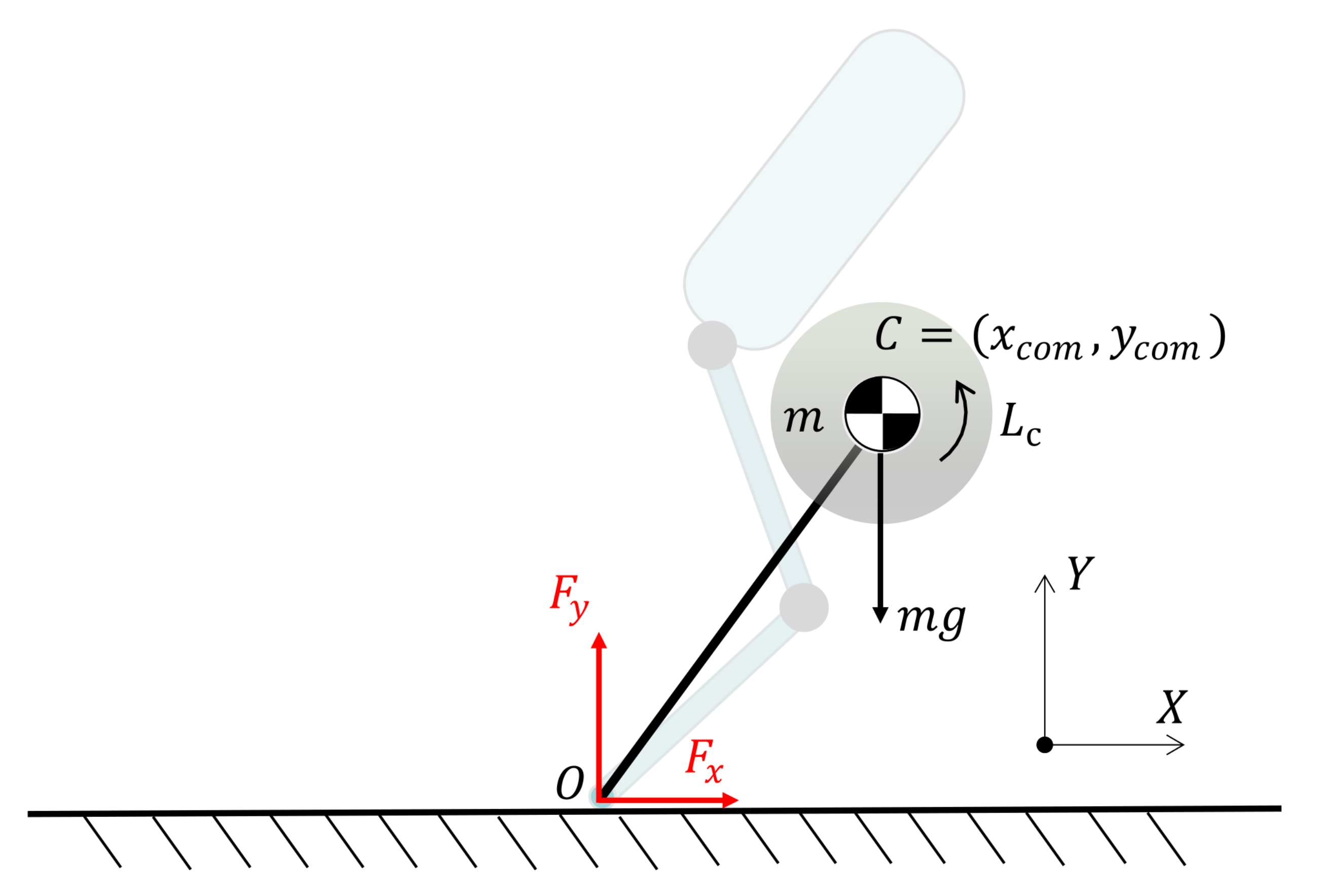
2.1. Model Configuration

In studying the balance problem, the robot model is considered to be a three-link rigid body comprising a torso, thigh and calf in the sagittal plane (as shown in Figure 2). Floating-base coordinates, $q_b={\left[x_b,y_b\right]}^T$, are used to describe the distance between the hip and ground. The robot’s posture is described by the posture coordinates $q_p={\left[\theta ,q_1,q_2\right]}^T$. The coordinates of the whole model are denoted $q={\left[x_b,y_b,\theta ,q_1,q_2\right]}^T$.

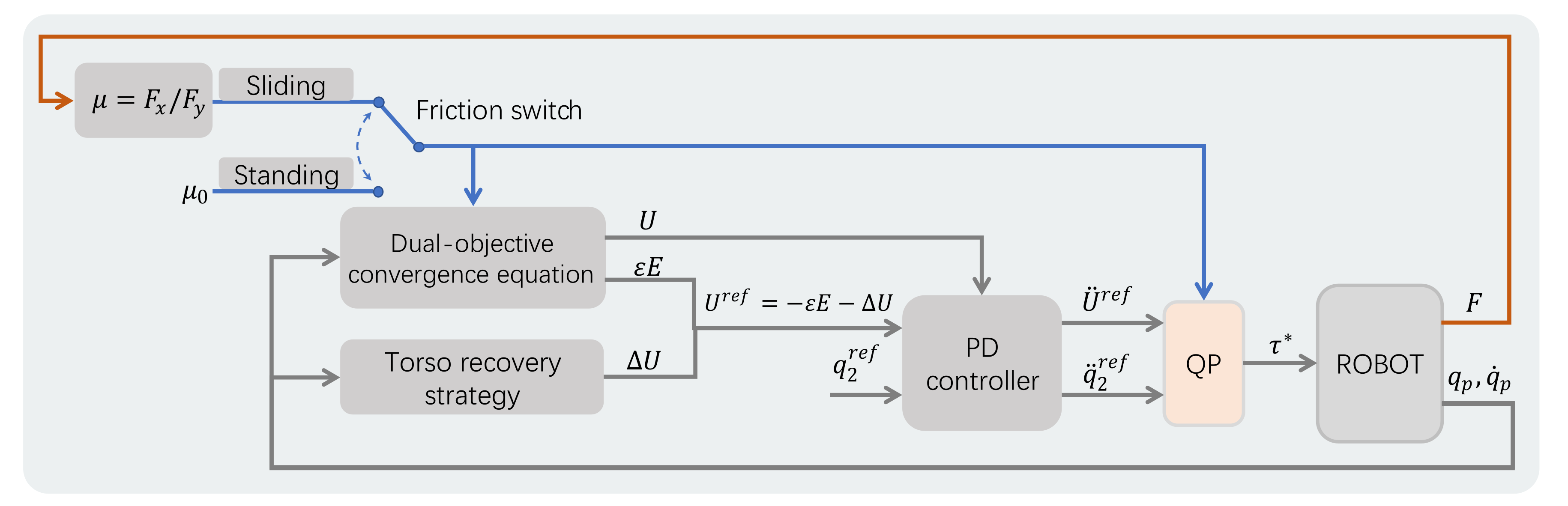
2.2. Dual-Objective Convergence Equation

To maintain a stable posture during sliding or standing, the derivative of the posture coordinate $\dot{q_p}={\left[\dot{\theta },\dot{q_1},\dot{q_2}\right]}^T$ should converge to zero. However, with one degree of under-actuation, the point-foot model, which has only two actuating joints at the hip and knee, is unable to drive these variables to zero directly. To control more variables with fewer DoFs, we design a virtual generalized velocity variable $E=J_E\left(q_p\right)\dot{q_p}$ as the posture stability criterion. We then use the variable to construct the dual-objective convergence equation:

$$\dot{E}=J_E\ddot{q_p}+{\dot{J}}_E\dot{q_p}=U\left(q_p\right)·P\left(q_p,\dot{q_p},\ddot{q_p}\right),$$

(1)

where $J_E\left(q_p\right)\in R^{1\times 3}$ is the matrix of the mapping from the derivative of the posture coordinate $\dot{q_p}$ to the posture stability criterion E, $U\left(q_p\right)\in R$ is a generalized coordinate that represents the equilibrium variable, and $P\left(q_p,\dot{q_p},\ddot{q_p}\right)\in R$ is an instantaneous constraint, the value of which can be controlled directly using $\ddot{q_p}$. We treat U as the controlled variable. If U can track E according to

$$U\left(q_p\right)=U^{ref}=-\epsilon E$$

(2)

with

$$P\left(q_p,\dot{q_p},\ddot{q_p}\right)>0,$$

(3)

then the posture stability criterion E can converge to zero over time. Here, $\epsilon \in R$ is the dual-objective proportional constant and $U^{ref}$ is regarded as a reference equilibrium target for $U\left(q_p\right)$. Furthermore, in the case that $E\equiv 0$ and $P>0$, U can be quantificationally calculated using (1), we have

$$U\left(q_p\right)\equiv 0.$$

(4)

Therefore, the first derivative of U is written as

$$\dot{U}=J_U\dot{q_p}=0,$$

(5)

where $J_U\left(q_p\right)\in R^{1\times 3}$ is the Jacobian matrix of $U\left(q_p\right)$. Therefore, through the dual-objective convergence equation, the stabilization of E and $\dot{U}$ can be realized simultaneously while controlling only one variable, U. This approach can thus stabilize more variables than the number of DoFs of the robot. The method of formulating the dual-objective convergence equation and the QP optimization controller for tracking $U^{ref}$ are discussed in later sections.

2.3. Convergence Equation for Sliding

Suppose that the robot slides at a high speed on the ground with constant friction $\mu$. A flywheel inverted-pendulum model is established to mathematically describe the trajectory of the CoM. As shown in Figure 3, point $C={\left[x_{com},y_{com}\right]}^T$ denotes the coordinates of the CoM, m is the total mass of the robot, and $L_c$ is the total angular momentum of all rigid bodies around the CoM. The magnitude of the gravitational action is $mg$. $F_x$ and $F_y$ are the x-axis and y-axis components of the contact force.

Because the rate of change of the centroidal angular momentum depends on the sum of torque around the CoM generated by the contact forces, the mathematical expression of the flywheel inverted-pendulum model is established as

$${\dot{L}}_c=y_{com}{F}_x-x_{com}{F}_y.$$

(6)

According to Coulomb’s law of friction, the contact force of the robot during sliding is

$$F_x={-\mu F}_y.$$

(7)

$F_y$ can be expressed as the acceleration of the CoM:

$$F_y=m\left({\ddot{y}}_{com}+g\right)=m\left(J_y\left(q_p\right)\ddot{q_p}+{\dot{J}}_y\left(q_p,\dot{q_p}\right)\dot{q_p}+g\right),$$

(8)

where $J_y\left(q_p\right)\in R^{1\times 3}$ is the Jacobian matrix of the y-axis component of the CoM. By substituting (7) and (8) into (6), the flywheel pendulum model is rewritten as

$${\dot{L}}_c=-\left({\mu y}_{com}+x_{com}\right)m\left(J_y\ddot{q_p}+{\dot{J}}_y\dot{q_p}+g\right).$$

(9)

Comparing the forms between (1) and (9), the dual-objective convergence equation for the sliding process is constructed as

$$E_{sl}=L_c,$$

(10)

$$U_{sl}\left(q_p\right)=-\left({\mu y}_{com}+x_{com}\right),$$

(11)

$$P_{sl}\left(q_p,\dot{q_p},\ddot{q_p}\right)=m\left(J_y\ddot{q_p}+{\dot{J}}_y\dot{q_p}+g\right),$$

(12)

where $E_{sl}$ is the posture stability criterion in sliding, $U_{sl}\left(q_p\right)$ describes the relation between the equilibrium variable and the CoM, and $P_{sl}\left(q_p,\dot{q_p},\ddot{q_p}\right)$ is the instantaneous constraint, which equals the y-axis component of the contact force.

Please note that (6) is tenable for any ground situation, while (7) is only suitable for horizontal ground. We suppose that the ground is flat with a constant friction coefficient ${\mu }_0$, but at a certain angle ${\theta }_g$ to the horizontal plane. The relation between $F_x$ and $F_y$ can be rewritten as

$$F_x={-{\mu }^{*}F}_y,$$

(13)

where

$${\mu }^{*}=tan\left({tan}^{-1}\left(\mu \right)+{\theta }_g\right).$$

(14)

During the actual sliding of the robot, ${\theta }_g$ is difficult to measure. However, ${\mu }^{*}$ can be estimated by measuring the actual contact force $F_x^{*}$ and $F_y^{*}$ at the feet:

$${\mu }^{*}=-\frac{F_x^{*}}{F_y^{*}}.$$

(15)

In this way, the convergence method can adapt to uneven ground with the replacement of $\mu$ in (11) with ${\mu }^{*}$.

2.4. Convergence Equation for Standing

When the robot stands on ground that provides a sufficient frictional force, the vertical force acting on the robot satisfies Equation (8) but the horizontal force acting on the robot is determined by the horizontal acceleration of the robot. When the robot no longer slides on the ground, $F_x$ can be obtained according to

$$F_x=m{\ddot{x}}_{com}=m\left(J_x\left(q_p\right)\ddot{q_p}+{\dot{J}}_x\left(q_p,\dot{q_p}\right)\dot{q_p}\right).$$

(16)

Considering that $F_x$ and $F_y$ can be expressed by Equations (8) and (16), the flywheel inverted-pendulum Equation (6) can be rewritten as

$${\dot{L}}_x+m\left(x_{com}{\ddot{y}}_{com}-y_{com}{\ddot{x}}_{com}\right)=-x_{com}mg.$$

(17)

According to the standard form of the dual-objective convergence equation in Equation (1), the convergence equation in the standing process is constructed as

$$E_{st}=L_c+m\left(x_{com}{\dot{y}}_{com}-y_{com}{\dot{x}}_{com}\right),$$

(18)

$$U_{st}\left(q_p\right)=-x_{com},$$

(19)

$$P_{st}=mg>0,$$

(20)

where $E_{st}$,$U_{st}\left(q_p\right)$ denotes the standard forms of the dual-objective convergence equation. Meanwhile, $P_{st}$ is a positive constant that automatically satisfies the restriction in Equation (3).

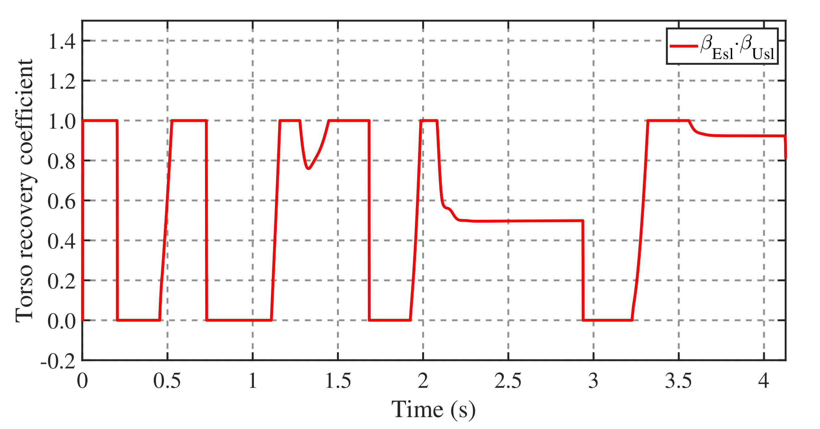
2.5. Torso Recovery Strategy

By controlling the equilibrium variable U to track the equilibrium target $U^{ref}$, both E and $\dot{U}$ are stabilized. To achieve whole-body control, however, all the controlled DoFs must be used up. Hence, the generalized coordinate of the joint of knee $q_2$ is expected to be another controlled variable that is used to drive the angle of the knee to a constant reference angle $q_2^{ref}$. By effectively controlling U and $q_2$, the robot will gradually tend to balance and eventually stay in some stationary posture, because the convergence of the triple variable (E, $\dot{U}$ and $q_2$) can be mapped to the convergence of the three-DoF posture coordinate $q_p$. However, while this method can stabilize the robot, it is unable to converge the torso to a desired angle. The following torso recovery strategy is thus adopted to adjust the angle of the upper body.

• First, reduce the difference (i.e., error) between U and $U^{ref}$ so that E begins to converge in the desired way.
• Then, wait for the amplitude of E to gradually decrease to within a permissible range, which indicates that the robot enters a stable state.
• Finally, add an equilibrium offset $\Delta U$ to the desired equilibrium target $U^{ref}$ according to the feedback states of the torso. Therefore, the angle of the torso $\theta$ gradually recovers to the reference value.

To put the above strategy into practice, we designed a torso position feedback control method based on coefficient regulation, which is summarized as

$${\beta }_E=clamp\left(\frac{{\rho }_E-\left|E_n\right|}{\Delta {\rho }_E},0,1\right),$$

(21)

$${\beta }_U=clamp\left(\frac{{\rho }_U-\left|U_{n-1}^{ref}-U_{n-1}\right|}{\Delta {\rho }_U},0,1\right),$$

(22)

$$\Delta U_{\theta }=clamp\left(\frac{{\theta }^{ref}-\theta }{{\Delta }_{\theta }},-1,1\right),$$

(23)

$$\Delta U_{\dot{\theta }}=clamp\left(\frac{\dot{\theta }}{{\Delta }_{\dot{\theta }}},-1,1\right),$$

(24)

$$\Delta U_n={\beta }_E·{\beta }_U·\left({\beta }_{\theta }·\Delta U_{\theta }+{\beta }_{\dot{\theta }}·\Delta U_{\dot{\theta }}\right),$$

(25)

$$clamp\left(x,a,b\right)=\left\{\begin{array}{ccc}x,& & a<x<b\\ a,& & x<a\\ b,& & x>b\end{array}\right..$$

(26)

Here, n is the current control period. ${\beta }_E$ is the coefficient regulator of the posture balance criterion E, and it increases linearly from 0 to 1 as $\left|E_n\right|$ decreases from ${\rho }_E$ to ${\rho }_E-\Delta {\rho }_E$. ${\beta }_U$ is the same regulator as ${\beta }_E$, and the product of these two coefficients ${\beta }_E$${\beta }_U$ is the torso recovery coefficient. $\Delta U_{\theta }$ and $\Delta U_{\dot{\theta }}$ are the proportional and differential limiters, ${\Delta }_{\theta }$ and ${\Delta }_{\dot{\theta }}$ are the linear ranges of the limiters. ${\beta }_{\theta }$ and ${\beta }_{\dot{\theta }}$ are the proportional and differential constants of the feedback controller. $\Delta U_n$ is the equilibrium offset of the current control period. The parameters in the equation are represented by a constant vector $K_{\theta }=\left[{\rho }_E,\Delta {\rho }_E,{\rho }_U,\Delta {\rho }_U,{\Delta }_{\theta },{\Delta }_{\dot{\theta }},{\beta }_{\theta },{\beta }_{\dot{\theta }}\right]$. After introducing the torso control strategy, compared with Equation (2), the equilibrium target $U^{ref}$ is modified as

$$U_n^{ref}=-\epsilon E-\Delta U_n.$$

(27)

3. QP Controller with Multiple Constraints

3.1. Qp Process

The QP method is widely used in the multi-task optimization of humanoid robots. In our control system (as shown in Figure 4), the control process starts with the friction switch, where the friction coefficient is calculated according to $\mu =F_x/F_y$ when the robot is sliding and is set as a reference value ${\mu }_0$ when the robot is standing. Next, the current equilibrium variable U and the equilibrium target $\epsilon E$ are calculated using the dual-objective convergence equation, where the equilibrium target is modified by the torso recovery strategy to obtain $U^{ref}$. A PD controller is then applied to calculate the reference input ${\ddot{U}}^{ref}$ and ${\ddot{q}}_2^{ref}$ according to the control tasks $U^{ref}$ and $q_2^{ref}$. Finally, the QP optimizer is used to solve optimal torque ${\tau }_{*}$ subject to the contact and dynamic constraints. By setting $u={\left[\ddot{q},\tau ,{\delta }_U,{\delta }_q\right]}^T$ as the optimization variable, the optimization problem for the control system is described as

$$u^{*}=\underset{u}{argmin}{u}^{T}Hu+Fu,$$

(28)

$$s.t.\left\{\begin{array}{ccc}{A}_X^{D}u=b_X^D& & \left(dynamicConstrain\right)\\ A_X^{c}u<b_X^c& & \left(contactConstrain\right)\\ \begin{array}{c}\ddot{U}={\ddot{U}}^{ref}+{\delta }_U\\ {\ddot{q}}_2={\ddot{q}}_2^{ref}+{\delta }_q\end{array}& & \left(controlConstrain\right)\\ u_{min}<u<u_{max}& & \left(variablelimit\right)\end{array}\right..$$

(29)

In the optimization problem, both the dynamic equation and contact inequation are strict constraints. For the solvability of QP, ${\delta }_U$ and ${\delta }_q$ are introduced into the control constraints as relaxation factors using a method similar to that adopted in [32]. Considering the minimization of $\left|{\delta }_U\right|$ and $\left|{\delta }_q\right|$, we introduce two positive weight coefficients, ${\rho }_U$ and ${\rho }_q$, to establish the cost function:

$$\underset{u}{min}{\rho }_U{\delta }_U^2+{\rho }_q{\delta }_q^2.$$

(30)

The matrix H and vector F of the cost function in the QP problem are thus set as

$$H=diag\left[0^{1\times 7},{\rho }_U,{\rho }_q\right],$$

(31)

$$F=0^{9\times 1},$$

(32)

and the standard form of the control constrain is constructed as

$$A_{i}u=b_i,$$

(33)

where

$$A_i=\left[\begin{array}{cccc}\begin{array}{c}{0}^{1\times 2}\\ 0^{1\times 4}\end{array}& \begin{array}{c}{J}_U\\ 1\end{array}& \begin{array}{c}{0}^{2\times 2}\\ 0^{2\times 2}\end{array}& \begin{array}{cc}-1& 0\\ 0& -1\end{array}\end{array}\right],$$

(34)

$$b_i=\left[\begin{array}{c}{\ddot{U}}^{ref}-{\dot{J}}_U\dot{q_p}\\ {\ddot{q}}_2^{ref}\end{array}\right].$$

(35)

3.2. PD Controller

The QP method can handle the conflict between the constraints and reference inputs to calculate a possible solution of the control variables. However, the control variables $\ddot{U}$ and ${\ddot{q}}_2$ solved by QP should not only be able to track $U^{ref}$ and $q_2^{ref}$ effectively but also have appropriate amplitudes. Therefore, a double-loop PD controller is adopted to generate the reference input:

$${\dot{X}}^{ref}=K_{p1}·clamp\left(\frac{X^{ref}-X}{{\Delta }_X},-1,1\right)-K_{d1}·clamp\left(k_c\dot{X},-1,1\right),$$

(36)

$${\ddot{X}}^{ref}=K_{p2}·clamp\left(\frac{{\dot{X}}^{ref}-\dot{X}}{{\Delta }_{\dot{X}}},-1,1\right),$$

(37)

where X stands for $U_{sl}$, $U_{st}$ and $q_2$. Thus, the first and second derivatives of the control variables U and $q_2$ are limited to a certain amplitude through $K_{p1}$, $K_{d1}$ and $K_{p2}$. Additionally, the sensitivity of the controller can be adjusted by ${\Delta }_X$ and ${\Delta }_{\dot{X}}$. The PD parameters are represented by the constant vector $K_X=\left[K_{p1},{\Delta }_X,K_{d1},k_c,K_{p2},{\Delta }_{\dot{X}}\right]$.

3.3. Dynamic Constraints

The dynamics of the model with the configuration described in Section 2.1 are expressed by the Euler–Lagrange equation:

$$D\left(q\right)\ddot{q}+C\left(q,\dot{q}\right)\dot{q}+G\left(q\right)=B\tau +{J\left(q\right)}^{T}F,$$

(38)

where $D\left(q\right)\in R^{5\times 5}$ is the inertia matrix, $C\left(q,\dot{q}\right)\in R^{5\times 5}$ is the matrix of Coriolis and centrifugal terms, $G\left(q\right)\in R^5$ is the gravity vector, $\tau \in R^2$ is the torque of joints, and $B\in R^{5\times 2}$ is the generalized force mapping matrix. For a point-foot model, $F=\left[F_x,F_y\right]$ is a vector comprising the x-axis and y-axis components of the contact force, and $J\left(q\right)\in R^{5\times 2}$ is the Jacobian of coordinates of the contact point.

During the process of high-speed sliding, the contact force needs to satisfy (7) and (8) so that the dynamics Equation (38) can be rewritten as

$$D_{sl}\ddot{q}+C_{sl}\dot{q}+G_{sl}=B\tau ,$$

(39)

where

$$D_{sl}=D\left(q\right)-{mJ\left(q\right)}^T\left[\begin{array}{cc}{0}^{2\times 2}& \begin{array}{c}-\mu J_y\\ J_y\end{array}\end{array}\right],$$

(40)

$$C_{sl}=C\left(q,\dot{q}\right)-{mJ\left(q\right)}^T\left[\begin{array}{cc}{0}^{2\times 2}& \begin{array}{c}-\mu {\dot{J}}_y\\ {\dot{J}}_y\end{array}\end{array}\right],$$

(41)

$$G_{sl}=G\left(q\right)-{mJ\left(q\right)}^T\left[\begin{array}{c}-\mu g\\ g\end{array}\right].$$

(42)

Similarly, according to Equations (8) and (16), the dynamic equation for standing is rewritten as

$$D_{st}\ddot{q}+C_{st}\dot{q}+G_{st}=B\tau ,$$

(43)

where

$$D_{st}=D\left(q\right)-{mJ\left(q\right)}^T\left[\begin{array}{cc}{0}^{2\times 2}& \begin{array}{c}{J}_x\\ J_y\end{array}\end{array}\right],$$

(44)

$$C_{st}=C\left(q,\dot{q}\right)-{mJ\left(q\right)}^T\left[\begin{array}{cc}{0}^{2\times 2}& \begin{array}{c}{\dot{J}}_x\\ {\dot{J}}_y\end{array}\end{array}\right],$$

(45)

$$G_{st}=G\left(q\right)-{mJ\left(q\right)}^T\left[\begin{array}{c}0\\ g\end{array}\right].$$

(46)

Using X to represent $sl$ and $st$, the dynamic Equations (39) and (43) are rewritten in the standard form of dynamic constraints in QP:

$$\left[\begin{array}{ccc}{D}_X& -B& 0^{1\times 2}\end{array}\right]u=-C_X\dot{q}-G_X.$$

(47)

3.4. Contact Constraints

The QP controller should be subject to (3) so that the validity of the dual-objective convergence equation is maintained. However, $P_{st}$ in Equation (20) is a positive constant and $P_{sl}$ in Equation (12) is equal to the vertical contact force $F_y$. Therefore, the constraint in (3) can be included in the contact constraints.

3.4.1. Contact Constraint in Sliding

During the sliding process, in addition to satisfying the constraint in (12), $F_y$ also needs to be limited within a certain range, which not only ensures that the robot’s sole is in full contact with the ground but also avoids an excessive contact force. Therefore, the constraint inequation ${\Phi }_{sl}$ is established:

$${\Phi }_{sl}:{{\alpha }_{min}mg<F}_y<{\alpha }_{max}mg,$$

(48)

where ${\alpha }_{min}$ and ${\alpha }_{max}$ are the max and min proportions of the vertical contact force. By dividing both sides of this inequality ${\Phi }_{sl}$ by the robot’s total mass m, the contact constraint is expressed as

$$\left[\begin{array}{ccc}{0}^{2\times 2}& \begin{array}{c}{-J}_y\\ J_y\end{array}& 0^{2\times 4}\end{array}\right]u<\left[\begin{array}{c}{\dot{J}}_y\dot{q_p}+g-{\alpha }_{min}g\\ -{\dot{J}}_y\dot{q_p}-g+{\alpha }_{max}g\end{array}\right].$$

(49)

3.4.2. Contact Constraint in Standing

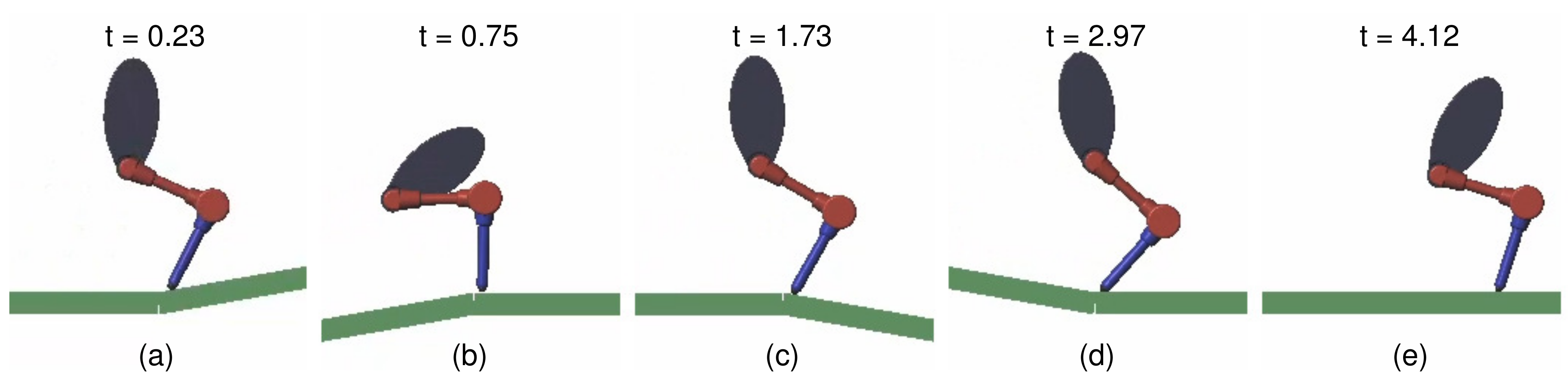
Standing on the ground without slipping requires the contact force to be inside the friction cone. Considering the same conditions as for ${\Phi }_{sl}$, the constraint equation ${\Phi }_{st}$ can be derived as

$${\Phi }_{st}:\left\{\begin{array}{c}\\ {{\alpha }_{min}mg<F}_y<{\alpha }_{max}mg\\ \begin{array}{c}\\ -\mu F_y<F_x<\mu F_y\end{array}\end{array}\right..$$

(50)

Similar to inequation (49), ${\Phi }_{st}$ can be converted to a contact constraint inequation:

$$\left[\begin{array}{ccc}{0}^{4\times 2}& \begin{array}{c}{-J}_y\\ J_y\\ -\mu J_y-J_x\\ -\mu J_y+J_x\end{array}& 0^{4\times 4}\end{array}\right]u<\left[\begin{array}{c}{\dot{J}}_y\dot{q_p}+g-{\alpha }_{min}g\\ -{\dot{J}}_y\dot{q_p}-g+{\alpha }_{max}g\\ {\dot{J}}_x\dot{q_p}+\mu {\dot{J}}_y\dot{q_p}+\mu g\\ -{\dot{J}}_x\dot{q_p}+\mu {\dot{J}}_y\dot{q_p}+\mu g\end{array}\right].$$

(51)

4. Results

We use Simscape Multibody software to verify the control methods mentioned above. Simscape Multibody is a Simulink toolbox for physical multibody modeling that provides a simulation environment for three-dimensional mechanical systems. To verify the applicability of the above balance control method, we design the bipedal rigid body structure by linking the trunk, thigh and calf through revolute joint blocks. The input to a joint is a torque while the output of a joint is an angle and angular velocity. The floating coordinates of the robot comprise a two-DoF prismatic joint and one-DoF revolute joint and are fixed connection with the torso. For contact, we use the sphere-to-plane contact block in the Simscape Multibody Contact Forces Library [33] to build the contact model of the end of the calf and the ground. The control system runs at a frequency of 1 kHz, and the optimization problem is solved using the quadprog solver in the Optimization Toolbox for Matlab.

The simulation comprises three parts. The first part verifies the sliding capability on uneven ground with a low-friction coefficient. The second part verifies the sliding balance ability on ground with a variable friction coefficient. The third part verifies the standing balance recovery for a low-friction coefficient. The total mass of the model is 26.9 kg, with the mass of the torso being 15.6 kg and the mass of the leg being 11.3 kg. The mechanical parameters used in the simulation are presented in

Table 1. Mechanical parameters used in the simulation.

Description	Symbol	Value	Unit
torso mass	$m_0$	15.6	Kg
thigh mass	$m_1$	6.8	Kg
calf mass	$m_2$	4.5	Kg
torso inertia	$I_0$	0.49	Kg · m${}^2$
thigh inertia	$I_1$	0.11	Kg · m${}^2$
calf inertia	$I_2$	0.09	Kg · m${}^2$
torso length	$l_0$	0.40	m
thigh length	$l_1$	0.33	m
calf length	$l_2$	0.33	m

.

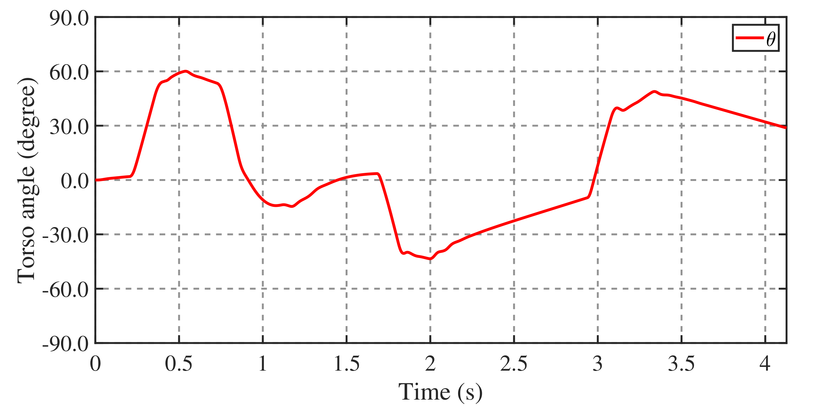
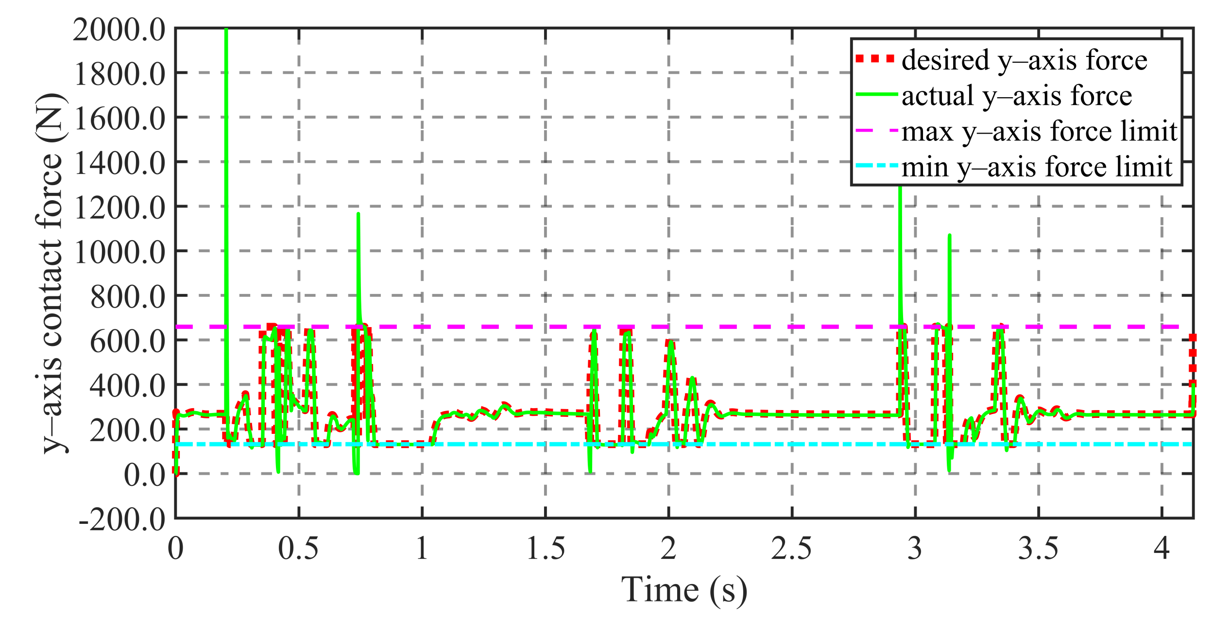
4.1. Balance in Sliding on Uneven Terrain

To verify the sliding capability on uneven terrain, a terrain including both uphill and downhill is modeled in the simulation scene. The robot is initially set to slide across the horizontal plane at an initial speed of 5 m/s and then slide into a trapezoidal terrain comprising an uphill, flat-top and downhill. The lengths of the uphill, flat-top and downhill sections are 2 m, the friction coefficient is 0.15, and the slope is 10 degrees. The robot is released from a balanced posture with the torso upright and the knees bent at 90 degrees. The parameters of the control system are given in

Table 2. Control parameters in sliding.

Description	Symbol	Value
dual-objective proportion	$\epsilon$	0.025
torso control parameter	$K_{\theta }$	[0.50, 0.25, 0.04, 0.02, 10$\pi$/180, 500$\pi$/180, 0.0125, 0.0156]
equilibrium variable PD parameter	$K_{U_{sl}}$	[2.5, 0.02, 3.0, 0.5, 50.0, 1.0]
knee PD parameter	$K_{q_2}$	[$\pi$, 10$\pi$/180, 1.5$\pi$, 0.5, 20$\pi$, 200$\pi$/180]
equilibrium variable relaxations weight in QP	${\rho }_{U_{sl}}$	1000
knee relaxations weight in QP	${\rho }_{q_2}$	1
max Vertical contact force proportion	${\alpha }_{max}$	2.5
min Vertical contact force proportion	${\alpha }_{min}$	0.5

and the friction coefficient of the control system is estimated according to Equation (15) during the sliding. Figure 5 shows snapshots of the sliding simulation when the slope changes and the sliding stops. The sliding slope changes at 0.23, 0.75, 1.73 and 2.97s, after which the robot adjusts its attitude and recovers to the torso recovery state. The simulated motion is shown in the supplemental video.

Figure 6 shows the results of the friction coefficient estimation. The estimated friction coefficient changes as the robot slides onto a new slope. On the uphill and downhill, the estimated friction coefficient finally stabilizes at 0.338 and −0.025, which correspond to ground angles of 10.1 and −10.0 degrees estimated using Equation (14). Therefore, the friction coefficient estimated by the contact force effectively compensates for the ground slope angle.

Figure 7 shows the tracking result for the equilibrium variable. Abrupt changes in the estimated friction coefficient led to mutations in the equilibrium variable. There are a total of four mutations in the simulation, and the time from mutation to a reduction in the tracking error to less than ${\rho }_U-\Delta {\rho }_U$ (the maximum allowable error in Equation (22) for fully activating the equilibrium buffer) is 0.14, 0.12, 0.12 and 0.18 s. This result indicates that the dynamics-based control system can quickly converge from an unbalanced state to a stable torso recovery state.

Figure 8 shows the trajectory of the postural stability criterion. The tracking error of $U_{sl}$ will increase when the slope angle changes. Therefore, the control state of the system will deviate from the dual-objective convergence state and the posture stability criterion will diverge. The maximum deviation amplitude of the postural stability criterion in the sliding process is 2.1 Kg · m${}^2$/s. At t = 2.2 to 2.9 s and at t = 3.6 s to the moment of that the robot stops, $E_{sl}$ maintains an offset of −0.38 kg · m${}^2$/s and 0.27 kg · m${}^2$/s, respectively. This is because the robot is in the torso recovery state, where the robot recovers its torso posture while maintaining the equilibrium position.

The trajectory of the torso recovery coefficient is shown in Figure 9. In the sliding process, the maximum time interval between the robot sliding to a new sliding angle and the torso recovery coefficient rising to 1 is 0.43 s. When the robot is in the torso recovery stage, the torso control strategy proposed in this article can adjust the ratio of the torso recovery coefficient to ensure that the amplitude of $E_{sl}$ will not diverge during the sliding process. Figure 10 shows the simulation result for the torso angle. During the sliding process, the torso angle is effectively controlled within 60 degrees.

When the robot is sliding rapidly and especially when the torso is swinging rapidly, a large Coriolis force will act on the robot’s leg. Through the contact constraint proposed in this article, the vertical contact force is limited to between 132 and 659 N as shown in Figure 11. This simulation demonstrates that the robot can quickly stabilize its posture and gradually adjust its torso angle on terrain with a variable sliding angle.

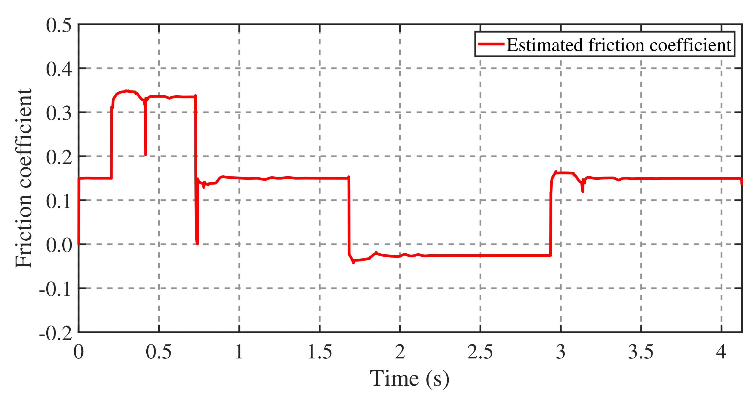
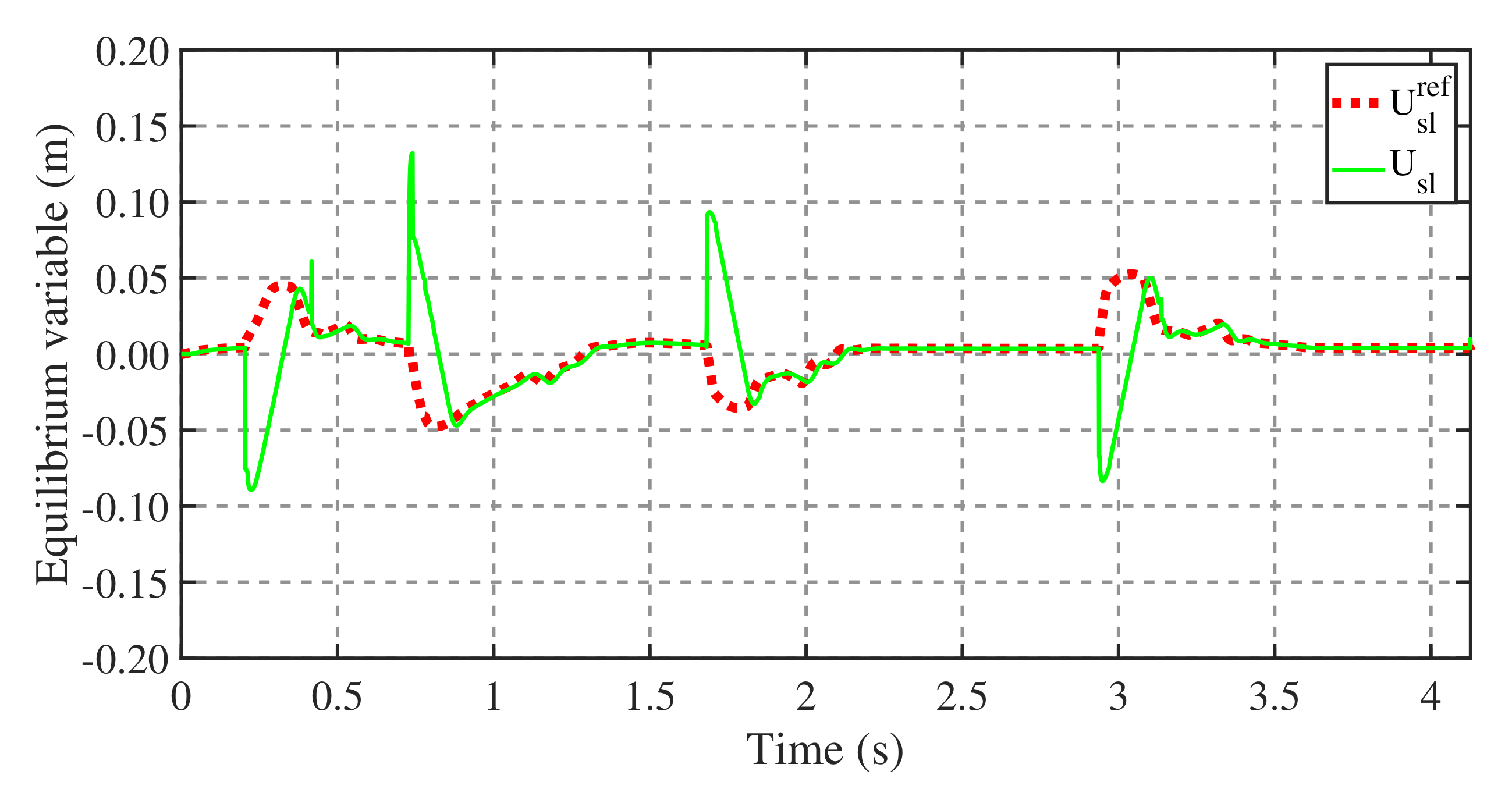
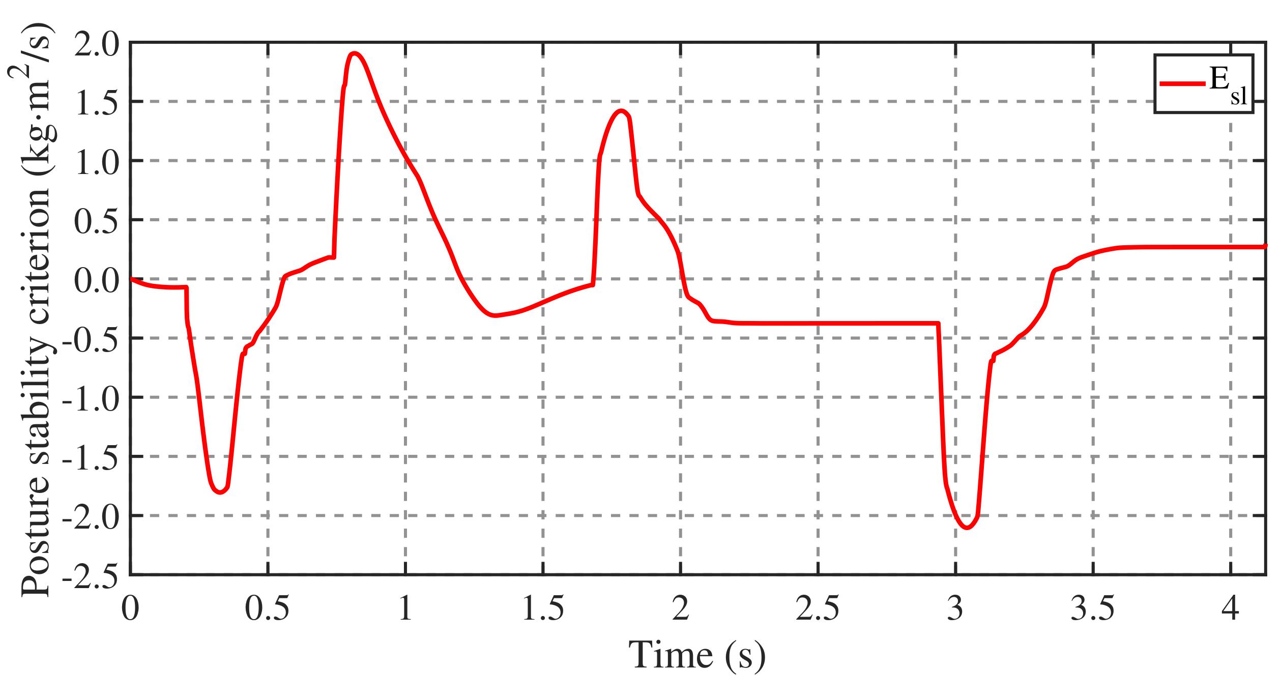
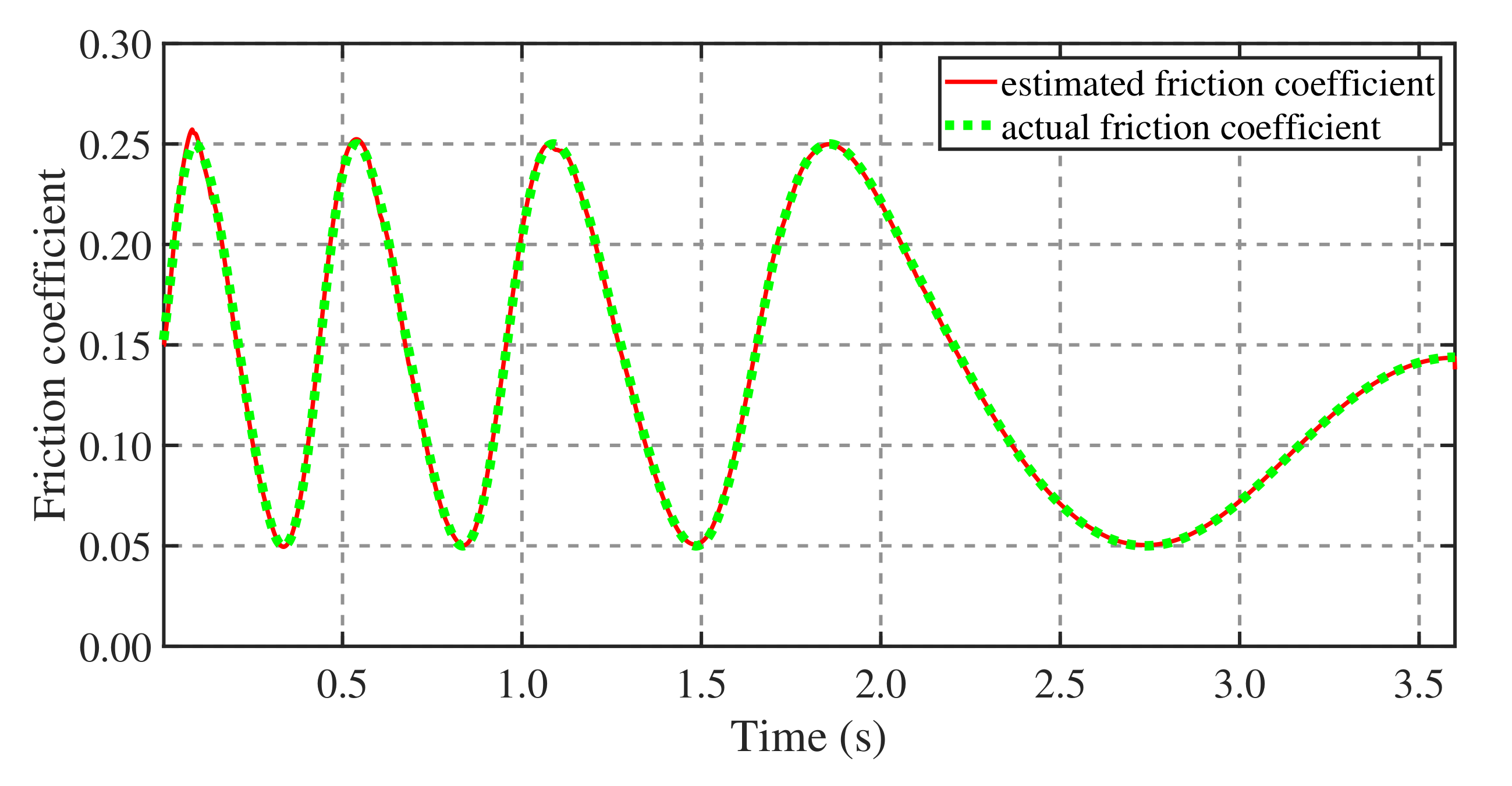
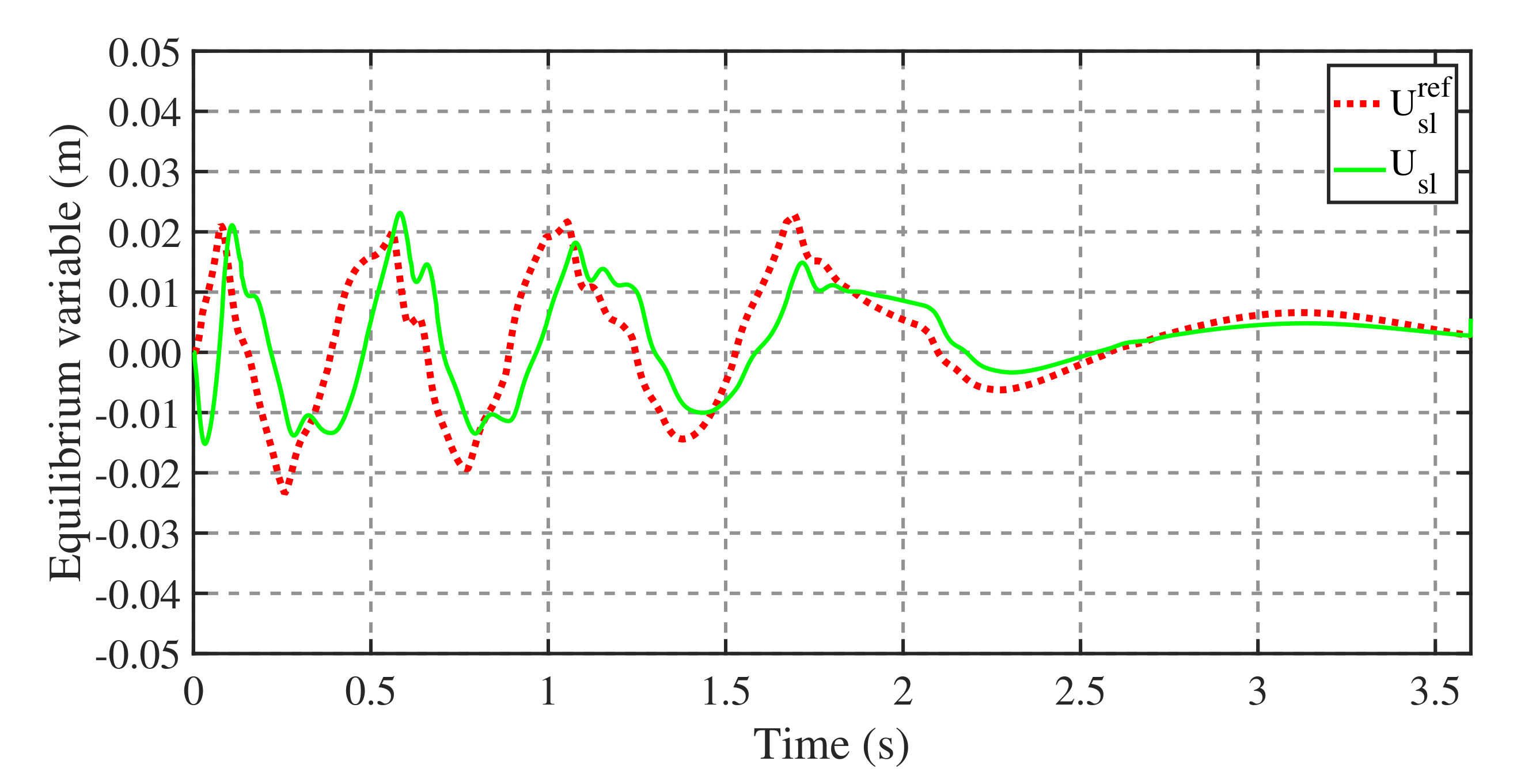
4.2. Balance Recovery on Terrain with a Variable Coefficient of Friction

The proposed control method has good adaptability on the ground with a variable friction coefficient. We use the same control parameters adopted in the previous experiment, and the friction coefficient of the ground is again estimated by measuring the contact force. In the simulation, the robot is released from the equilibrium position at a speed of 5 m/s. The friction coefficient of the ground is set as a sinusoidal function of the ground length with a magnitude range of 0.05 to 0.25. The equation for the friction coefficient is

$${\mu }_{ground}=0.15+0.1\times sin\left(2\pi \times \frac{groundlength}{2}\right).$$

Figure 12 shows the trajectories of the estimated friction coefficient and the actual friction coefficient. With the deceleration of the robot’s sliding, the fluctuating frequency of the friction coefficient gradually decreases, and the robot finally stops sliding after 3.6 s. Figure 13 shows the tracking result for the equilibrium variable. The tracking error gradually decreases as the sliding decelerates. The tracking error during the sliding has a maximum value of 0.024 m and decreases to 0.005 m at 1.48 s before the sliding stops. Figure 14 shows the trajectory of the robot’s torso angle. Throughout the sliding process, the robot’s torso angle remains within 20 degrees. The simulation results show that the control method proposed in this article can maintain the balance of the robot on terrain that has a continuous change in the friction coefficient.

4.3. Balance Recovery in Standing

We use the proposed method to realize self-balancing when the robot stands on ground with a low-friction coefficient consistent with the first case of simulation. The control parameters of the robot are given in

Table 3. Control parameters in standing.

Description	Symbol	Value
dual-objective proportion	$\epsilon$	0.01
torso control parameter	$K_{\theta }$	[1.0, 0.5, 0.02, 0.01, 10$\pi$/180, 1000$\pi$/180, 0.002, 0.003]
equilibrium variable PD parameter	$K_{U_{st}}$	[1.0, 0.02, 1.5, 1.5, 9.8, 0.2]
knee PD parameter	$K_{q_2}$	[$\pi$, 10$\pi$/180, 1.5$\pi$, 0.5, 20$\pi$, 200$\pi$/180]
equilibrium variable relaxations weight in QP	${\rho }_{U_{st}}$	1
knee relaxations weight in QP	${\rho }_{q_2}$	1
max Vertical contact force proportion	${\alpha }_{max}$	2.5
min Vertical contact force proportion	${\alpha }_{min}$	0.5

. Meanwhile, to verify the control performance, we set an x-axis offset of the CoM of 0.02 m and release the robot in a static posture. Figure 15 shows snapshots of the simulation video. On the horizontal ground, the robot stably recovers its torso without slipping and finally restores its torso to a vertical posture after 6.0 s.

Figure 16 shows the tracking results for the equilibrium variable when the robot is standing. The equilibrium variable reaches a maximum positive deviation of 0.012 m at t = 0.33 s and converges to within 0.001 m at t = 0.66 s. Figure 17 shows the torso angle trajectory. At t = 0.5 s, the torso angle reaches a maximum deflection angle of 78 degrees, and the torso angle is then in a stable convergence state. For the underactuated robot in the standing state, the CoM adjustment needs to be realized by rotating the torso, and the proposed control method provides an efficient stability criterion, so that the torso enters the convergence state after a major overshoot, thus avoiding the reciprocating swing of the torso. Figure 18 shows the expected force, actual force and friction limit of the model in the horizontal direction. In the case of standing on low-friction terrain, the horizontal friction falls to 85 N and is limited to the allowable range by the friction constraint in this article. The simulation demonstrates that the method proposed in this article can effectively solve the problem of a foot slipping as a result of an adjustment of the CoM when a robot stands on terrain with a low-friction coefficient, and that it can control the horizontal contact force within the limit of friction.

5. Discussion

In this article, we introduced a novel dual-objective convergence method for constructing the balance controller in sliding and standing states. Simulation demonstrated that the controller has good performance in both states. The dual-objective convergence equation was constructed using the flywheel inverted-pendulum model, and the balance criterion of the point-foot sliding model is the central angular momentum, which is similar to the CMP criterion used for balance in the standing and walking of a humanoid. However, the CMP method emphasizes the active control of the position relationship between the CMP and CoM through ankle and hip strategies. In the case of the robot sliding on terrain with a constant friction coefficient, as in the first simulation in this article, the CMP maintains a certain angle with the CoM owing to the constant friction angle of the contact surface, which makes it difficult to change the positional relationship. In contrast, the dual-objective convergence method proposed in this article focuses on the adaptive adjustment of the equilibrium position by changing the robot’s posture to adapt to the change in angular momentum, which is suitable for sliding friction conditions. In addition, the dual-objective convergence equation can be established using the robot’s dynamics model or other models, while the physical meaning of the dual-objective convergence equation established using a flywheel inverted pendulum is more explicit and more convenient for tuning the control parameters.

For task tracking, on the one hand, the QP optimization method proposed in this article can effectively handle the limitation of the contact force, which is an important balance requirement for the robot when changing posture rapidly. In addition, the QP framework can easily extend constraints to meet further requirements for constraints on more complex terrain. However, the QP method is an instantaneous optimization, and owing to the lack of feed-forward information, a certain delay will occur during task tracking. It is predicted that adopting differential dynamic programming or nonlinear model predictive control will achieve a better tracking effect, but this will increase the computational occupancy of the control algorithm, which is problematic for a high-frequency real-time control system. In addition to our research, the underactuated point-foot structure requires a sufficient and appropriate mass and inertia configuration to achieve effective task control. The larger mass and inertia of the torso allow for a faster posture balance with a smaller torso rotation. In contrast, the excessively small mass and inertia of the torso may result in multiple turns of torso rotation during the posture balance control, and even lead to the failure of the control algorithm.

6. Conclusions

This article presented a control framework based on the dual-objective convergence method and quadratic programming optimization to realize the sliding balance of a point-foot bipedal model. It was demonstrated that the point-foot model can cover a ${10}^{\circ }$ trapezoidal terrain and maintain balance on flat ground with a sinusoidal friction coefficient between 0.05 and 0.25 (whereas a robot sliding on ice has a friction coefficient of around 0.1). The main contribution of this article is that we designed a dual-objective convergence equation for the balance control of an underactuated point-foot system. First, through the double-convergence equation, we provided a control system with an equilibrium target that can control several degrees of freedom of the robot system that is greater than the number of its own dimensions. Second, we used a torso recovery strategy based on coefficient regulation and torso state feedback control to adjust the equilibrium target, which allowed the torso to eventually return to its upright posture instead of remaining in any other position. Finally, the quadratic programming optimization was adopted to realize efficient task tracking under constraints of dynamics, friction and contact forces. Furthermore, by switching to the standing model to rebuild the convergence equation and additional standing constraints, the dual-objective convergence method could be extended to standing balance, where the simulation results show that the control model can recover from an unstable state with a center of mass offset of 0.02 m to a stable posture with an upright torso. The method will have good scalability when the research scope is extended to more point-foot motion scenes and other balance control platforms, which is conducive to building stability criteria, generating balance tasks, and adapting to environmental constraints. In future work, first, we will introduce reinforcement learning to investigate the adaptive equilibrium position adjustment method under unexpected and undefined loads. Second, we will use machine vision to estimate the robot’s sliding speed and thus establish the switching control of the process from sliding to standing. Third, we will conduct experiments with a physical robot platform, which will face practical challenges such as state estimation, execution error and mechanism limits. Finally, we expect to extend the application of our method to bipedal jumping and running control.

References

1. Westervelt, E.R.; Grizzle, J.W.; Chevallereau, C.; Choi, J.H.; Tokyo, L. Feedback Control of Dynamic Bipedal Robot Locomotion; CRC Press: Boca Raton, FL, USA, 2007. [Google Scholar]
2. Kajita, S.; Hirukawa, H.; Harada, K.; Yokoi, K. Introduction to Humanoid Robotics; Springer: Berlin/Heidelberg, Germany, 2014. [Google Scholar]
3. Kajita, S.; Tani, K. Study of dynamic biped locomotion on rugged terrain-theory and basic experiment. In Proceedings of the Fifth International Conference on Advanced Robotics’ Robots in Unstructured Environments, Pisa, Italy, 19–22 June 1991. [Google Scholar]
4. Zhao, J.; Gao, J.; Zhao, F.; Liu, Y. A search-and-rescue robot system for remotely sensing the underground coal mine environment. Sensors 2017, 17, 2426. [Google Scholar] [CrossRef] [Green Version]
5. Waldron, K.J. Mobility and controllability characteristics of mobile robotic platforms. In Proceedings of the IEEE International Conference on Robotics and Automation, St. Louis, MO, USA, 25–28 March 1985. [Google Scholar]
6. Zheng, Y.; Wang, H.; Li, S.; Liu, Y.; Oh, P. Humanoid robots walking on grass, sands and rocks. In Proceedings of the IEEE International Conference on Technologies for Practical Robot Applications, Woburn, MA, USA, 22–23 April 2013. [Google Scholar]
7. Quan, N.; Hereid, A.; Grizzle, J.W.; Ames, A.D.; Sreenath, K. 3D dynamic walking on stepping stones with control barrier functions. In Proceedings of the 2016 IEEE 55th Conference on Decision and Control (CDC), Las Vegas, NV, USA, 12–14 December 2016. [Google Scholar]
8. Jo, S.H.; Chu, J.U.; Lee, Y.J. Motion planning for biped robot with quad roller skates. In Proceedings of the 2008 International Conference on Control, Automation and Systems, Seoul, Korea, 14–17 October 2008; pp. 1173–1177. [Google Scholar]
9. Hashimoto, K.; Hosobata, T.; Sugahara, Y.; Mikuriya, Y.; Takanishi, A. Realization by Biped Leg-wheeled Robot of Biped Walking and Wheel-driven Locomotion. In Proceedings of the 2005 IEEE International Conference on Robotics and Automation, Barcelona, Spain, 18–22 April 2005; pp. 2970–2975. [Google Scholar]
10. Lahajnar, L.; Kos, A.; Nemec, B. Skiing robot-design, control, and navigation in unstructured environment. Robotica 2009, 27, 567–577. [Google Scholar] [CrossRef] [Green Version]
11. Abdallah, M.E.; Goswami, A. A Biomechanically Motivated Two-Phase Strategy for Biped Upright Balance Control. In Proceedings of the IEEE International Conference on Robotics and Automation, Barcelona, Spain, 18–22 April 2005. [Google Scholar]
12. Mosadeghzad, M.; Li, Z.; Tsagarakis, N.G.; Medrano-Cerda, G.A.; Dallali, H.; Caldwell, D.G. Optimal ankle compliance regulation for humanoid balancing control. In Proceedings of the IEEE/RSJ International Conference on Intelligent Robots and Systems, Tokyo, Japan, 3–7 November 2013; pp. 4118–4123. [Google Scholar]
13. Stephens, B. Integral control of humanoid balance. IEEE/RSJ International Conference on Intelligent Robots and Systems. In Proceedings of the 2007 IEEE/RSJ International Conference on Intelligent Robots and Systems, San Diego, CA, USA, 29 October–2 November 2007. [Google Scholar]
14. Macchietto, A.; Zordan, V.; Shelton, C.R. Momentum control for balance. Acm Transactions on Graphics. ACM Trans. Graph. 2009, 28, 1–8. [Google Scholar] [CrossRef]
15. Lee, S.H.; Goswami, A. A momentum-based balance controller for humanoid robots on non-level and non-stationary ground. Auton. Robot. 2012, 33, 399–414. [Google Scholar] [CrossRef]
16. Yoshida, Y.; Takeuchi, K.; Sato, D.; Nenchev, D. Postural balance strategies for humanoid robots in response to disturbances in the frontal plane. In Proceedings of the 2011 IEEE International Conference on Robotics and Biomimetics, Karon Beach, Thailand, 7–11 December 2011. [Google Scholar]
17. Goswami, A.; Kallem, V. Rate of change of angular momentum and balance maintenance of biped robots. In Proceedings of the IEEE International Conference on Robotics and Automation, New Orleans, LA, USA, 26 April–1 May 2004; pp. 3785–3790.
18. Stephens, B. Humanoid push recovery. In Proceedings of the IEEE-RAS International Conference on Humanoid Robots, Pittsburgh, PA, USA, 29 November–1 December 2007. [Google Scholar]
19. Mayr, J.; Gattringer, H.; Bremer, H. Bipedal balancing control based on the centroidal momentum pivot and the best COM-CMP regulator. In Proceedings of the IECON 2013-39th Annual Conference of the IEEE Industrial Electronics Society, Vienna, Austria, 10–13 Novemeber 2013; pp. 4061–4066. [Google Scholar]
20. Shafiee-Ashtiani, M.; Yousefi-Koma, A.; Mirjalili, R.; Maleki, H.; Karimi, M. Push Recovery of a Position-Controlled Humanoid Robot Based on Capture Point Feedback Control. In Proceedings of the 2017 5th RSI International Conference on Robotics and Mechatronics, Tehran, Iran, 25–27 October 2017; pp. 126–131. [Google Scholar]
21. Zutven, P.V.; Kostiand, D.; Nijmeijer, H. Foot placement for planar bipeds with point feet. In Proceedings of the 2012 IEEE International Conference on Robotics and Automation, Saint Paul, MN, USA, 14–18 May 2012; pp. 983–988. [Google Scholar]
22. Kim, D.; Thomas, G.; Sentis, L. A method for dynamically balancing a point foot robot. In Proceedings of the 2015 IEEE-RAS 15th International Conference on Humanoid Robots, Seoul, Korea, 3–5 November 2015; pp. 901–907. [Google Scholar]
23. Peng, S.J.; Shui, H.T.; Tao, S.; Ma, H.X. A novel stability criterion for underactuated biped robot. In Proceedings of the 2009 IEEE International Conference on Robotics and Biomimetics, Guilin, China, 19–23 December 2009; pp. 1912–1917. [Google Scholar]
24. Grasser, F.; D’Arrigo, A.; Colombi, S.; Rufer, A.C. Joe: A mobile, inverted pendulum. IEEE Trans. Ind. Electron. 2002, 49, 107–114. [Google Scholar] [CrossRef]
25. Ha, J.; Lee, J. Position control of mobile two wheeled inverted pendulum robot by sliding mode control. In Proceedings of the 2012 12th International Conference on Control, Automation and Systems, Jeju, Korea, 17–21 October 2012; pp. 715–719. [Google Scholar]
26. Huang, C.; Wang, W.; Chiu, C. Design and Implementation of Fuzzy Control on a Two-Wheel Inverted Pendulum. IEEE Trans. Ind. Electron. 2011, 58, 2988–3001. [Google Scholar] [CrossRef]
27. Jeong, S.; Takahashi, T. Wheeled inverted pendulum type assistant robot: Design concept and mobile control. Intell. Serv. Robot. 2008, 1, 313–320. [Google Scholar] [CrossRef]
28. Khatib, O. A unified approach for motion and force control of robot manipulators: The operational space formulation. IEEE J. Robot. Autom. 1987, 3, 43–53. [Google Scholar] [CrossRef] [Green Version]
29. Hutter, M.; Hoepflinger, M.; Remy, C.; Siegwart, R. Hybrid Operational Space Control for Compliant Legged Systems. In Proceedings of the Robotics science and systems VIII, Sydney, Australia, 9–13 July 2012; pp. 129–136. [Google Scholar]
30. Zafar, M.; Hutchinson, S.; Theodorou, E.A. Hierarchical optimization for Whole-Body Control of Wheeled Inverted Pendulum Humanoids. In Proceedings of the 2019 International Conference on Robotics and Automation, Montreal, QC, Canada, 20–24 May 2019; pp. 7535–7542. [Google Scholar]
31. Klemm, V.; Morra, A.; Gulich, L.; Mannhart, D.; Rohr, D.; Kamel, M.; Viragh, Y.; Siegwart, R. LQR-Assisted Whole-Body Control of a Wheeled Bipedal Robot With Kinematic Loops. IEEE Robot. Autom. Lett. 2020, 5, 3745–3752. [Google Scholar] [CrossRef]
32. Ames, A.D.; Powell, M. Towards the unification of locomotion and manipulation through control lyapunov functions and quadratic programs. Lect. Notes Control. Inf. Sci. 2013, 449, 219–240. [Google Scholar]
33. Steve, M. Simscape Multibody Contact Forces Library. 2020. Available online: https://github.com/mathworks/Simscape-Multibody-Contact-Forces-Library/releases/tag/20.2.5.0 (accessed on 20 November 2020).
Figure 1. Block diagram of the balance control framework. τ * is the optimized joint torque.
Applsci 11 04016 g001
Figure 2. Coordinates and structural configuration. X b and Y b are the x and y floating-base coordinates. θ is the angle between the y-axis of the world frame and the torso. q 1 and q 2 are the joint coordinates of the hip and knee. m, I and l are the mass, inertia and length of a rigid body.
Applsci 11 04016 g002
Figure 3. Flywheel inverted-pendulum model of the biped robot.
Applsci 11 04016 g003
Figure 4. Robot control system.
Applsci 11 04016 g004
Figure 5. Snapshots of sliding on uneven terrain: (a) sliding from the bottom to the uphill, (b) sliding from the uphill to the flat-top, (c) sliding from the flat-top to the downhill, (d) sliding from the downhill to the bottom, (e) sliding having stopped.
Applsci 11 04016 g005
Figure 6. Trajectory of the estimated friction coefficient when the robot slides on uneven terrain.
Applsci 11 04016 g006
Figure 7. Trajectory of the equilibrium variable when the robot slides on uneven terrain.
Applsci 11 04016 g007
Figure 8. Trajectory of the postural stability criterion when the robot slides on uneven terrain.
Applsci 11 04016 g008
Figure 9. Trajectory of the torso recovery coefficient when the robot slides on uneven terrain.
Applsci 11 04016 g009
Figure 10. Trajectory of the torso angle when the robot slides on uneven terrain.
Applsci 11 04016 g010
Figure 11. Vertical contact force when the robot slides on uneven terrain.
Applsci 11 04016 g011
Figure 12. Trajectory of the estimated friction coefficient when the robot slides on terrain with a variable friction coefficient.
Applsci 11 04016 g012
Figure 13. Trajectory of the equilibrium variable when the robot slides on terrain with a variable friction coefficient.
Applsci 11 04016 g013
Figure 14. Trajectory of the torso angle when the robot slides on terrain with a variable friction coefficient.
Applsci 11 04016 g014
Figure 15. Snapshots of the posture recovery when the robot stands on ground with a low-friction coefficient.
Applsci 11 04016 g015
Figure 16. Trajectory of the equilibrium variable when the robot is sliding.
Applsci 11 04016 g016
Figure 17. Trajectory of the torso angle when the robot is sliding.
Applsci 11 04016 g017
Figure 18. Horizontal contact force when the robot is sliding on terrain with a variable friction coefficient.
Applsci 11 04016 g018