Kinematic-Model-Free Redundancy Resolution Using Multi-Point Tracking and Control for Robot Manipulation

Abstract

Robots have been predominantly controlled using conventional control methods that require prior knowledge of the robots’ kinematic and dynamic models. These controllers can be challenging to tune and cannot directly adapt to changes in kinematic structure or dynamic properties. On the other hand, model-learning controllers can overcome such challenges. Our recently proposed model-learning orientation controller has shown promising ability to simultaneously control a three-degrees-of-freedom robot manipulator’s end-effector pose. However, this controller does not perform optimally with robots of higher degrees-of-freedom nor does it resolve redundancies. The research presented in this paper extends the state-of-the-art kinematic-model-free controller to perform pose control of hyper-redundant robot manipulators and resolve redundancies by tracking and controlling multiple points along the robot’s serial chain. The results show that with more control points, the controller is able to reach desired poses in fewer steps, yielding an improvement of up to 66%, and capable of achieving complex configurations. The algorithm was validated by running the simulation 100 times, and it was found that, in 82% of the times, the robot successfully reached the desired target pose within 150 steps.

1. Introduction

Conventional robot controllers require both the kinematic and dynamic models (heron cumulatively referred to as kinodynamic model) of the robot in order to perform accurate control [1]. These controllers require an accurate model of the robot. However, soft robots, morphing robots, malleable robots, transforming robots, and evolving robots can be challenging to model accurately and control. Model-based approaches have remained the dominant control method for over 50 years [2]. Model-based control of soft/continuum robots underperform because modeling these structures are achieved by means of approximations. Therefore, learning-based or model-free techniques may be preferred to overcome some of these challenges.

Recently, a new class of model-learning controllers emerged, showing promising ability to bypass the need for any prior robot model. These controllers directly learn a kinodynamic model online to control a robot. In our original work, the Encoderless controller [3] and Kinematic-Free controller [4], the end-effector position of a two-degree-of-freedom (2-degrees-of-freedom) robot manipulator was controlled in task space. The controller works by generating local linear models that represent the robot’s local kinodynamics, which are used to actuate the robot’s end effector towards a given target position. In our most recent work, the model-learning orientation controller [5] has successfully controlled the position and orientation of a 3-degrees-of-freedom robot manipulator’s end effector in task space without any predefined kinodynamic model of the robot. However, this controller underperforms, taking longer than required to converge to the desired pose, when higher-degrees-of-freedom robots are to be controlled, leaving redundancies unresolved, as well.

The Kinematic-Model-Free (KMF) Multi-Point controller presented in this paper extends the state-of-the-art kinematic-model-free orientation controller, enabling the control of hyper-redundant robot manipulators and resolving redundancies in these manipulators by tracking and controlling multiple points along the kinematic chain of such robots.

1.1. Contributions

The contributions of this papers are as follows: (1) the novel kinematic-model-free multi-point controller presented in this paper expands the state-of-the-art kinematic-model-free controller to control the pose of multiple points along a robot’s kinematic chain; (2) the controller allows for the control of robots with high degrees-of-freedom, scaling up from the 3-degrees-of-freedom manipulator in our previous work; and (3) the controller is also capable of resolving redundancies in highly redundant system, such as continuum robots.

1.2. Paper Structure

Section 2 introduces work related to the research presented in this paper. Section 3 summarizes the fundamental mathematical background required to understand the working principles of the novel kinematic-model-free multi-point controller. Section 4 introduces the proposed controller along with its mathematical equations. Section 5 presents experimental results. Finally, Section 6 concludes the paper.

2. Related Work

Model-based controllers have been the predominant method of control for robot manipulation. The Jacobian of a robot, which relates the joint velocities to the end-effector velocity, is calculated prior to control [6], after which it is controlled using forward and inverse kinematics [7]. Using such models imposes many limitations [8] and assumes the Denavit-Hartenberg parameters, that define the robots kinematics, to be static. One example of model-based control is visual servoing that uses an external camera to calculate the required end-effector velocity to reach a desired target [9]. However, this assumption falls apart in the case of soft robots, when robots are damaged, or when robots transform or evolve in any way, such as altering the end effector by changing its gripper. Therefore, model-based conventional controllers are accurate but not adaptable.

Other researchers performed model-free control by approximating a Jacobian that is later used to actuate a robot. Researchers in Reference [10] controlled a deformable manipulator and in Reference [11] controlled a soft manipulator by approximating its Jacobian model. Other researchers controlled a dynamically-undefined robot by first estimating the robot’s dynamic parameters and then controlled a robot using conventional methods [12]. Learning methods, such as motor babbling, that start with no predefined model of a robot’s kinodynamics are used to approximate a model to control robots [13]. Other researchers use machine learning [14] and reinforcement learning algorithms [15] to control robots.

On the other hand, researchers in Reference [16] directly controlled current motors to actuate an unmanned underwater vehicle by means of deterministic artificial intelligence where uncertainties are ignored by making use of first principles. Researchers in Reference [17] controlled a SCARA robot’s position through motor voltages using extended state observer to estimate system dynamics. Other researchers studied hybrid model-free and model-based approaches to increase the performance of robot navigation [18]. However, most of these learning approaches require encoder feedback for estimating the robot’s pose.

The classical kinematic-model-free position controllers, the Encoderless [3] and Kinematic-Free [4] controllers, do not require any prior model of the robot. They operate by generating psuedo-random actuation signals that actuate a planar 2-degrees-of-freedom robot’s joints causing a positional displacement on the robot’s end effector. The effect on the robot’s end effector is observed using an external camera and is recorded. The recorded data are then used to generate a local linear model that actuates the robot’s end effector towards a given target. Any discrepancies will re-trigger another exploratory phase. The classical kinematic-model-free controller was then extended to simultaneously control the position and orientation of a 3-degrees-of-freedom robot’s end effector [5] using locally-weighted dual quaternions. These kinematic-model-free controllers, however, are unable to resolve redundancies in redundant robots, such as manipulators with high degrees of freedom [19] and continuum robots [20].

3. Mathematical Background

3.1. Quaternions

Quaternions, introduced by Hamilton in 1844 [21], are extend the complex number system used to represent rigid-body rotations. A quaternion $\mathbf{q}$ is the sum of a scalar s and a vector $\mathbf{v}=(q_1,q_2,q_3)$:

$$\mathbf{q}=s+\mathbf{v}=s+q_1\mathbf{i}+q_2\mathbf{j}+q_3\mathbf{k},$$

(1)

where i, j, k are unit vectors pointing in the x, y, z directions.

The conjugate of a quaternion $\mathbf{q}$ is defined as:

$${\mathbf{q}}^{*}=s-\mathbf{v}=s-q_1\mathbf{i}-q_2\mathbf{j}-q_3\mathbf{k},$$

(2)

which is used to calculate the norm of a quaternion as follows:

$$\Vert \mathbf{q}\Vert =\sqrt{{\mathbf{q}}^{*}\mathbf{q}}.$$

(3)

Unit quaternions satisfy $s^2+q_1^2+q_2^2+q_3^2=1$ or simply $\Vert \mathbf{q}\Vert =1$.

More information on quaternions can be found in Reference [22].

3.2. Dual Quaternions

Dual quaternions, presented by Clifford in 1871 [23], are extend the dual number system. A dual quaternion $\widehat{\mathbf{q}}$ is defined as the sum of two quaternions:

$$\widehat{\mathbf{q}}=\mathbf{p}+ϵ\mathbf{q},$$

(4)

where $\mathbf{p}=s_p+{\mathbf{v}}_p$ is the real part, and $\mathbf{q}=s_q+{\mathbf{v}}_q$ is the dual part. The dual element $ϵ$ is nilpotent, i.e., ${ϵ}^2=0$.

The conjugate of a dual quaternion is defined as:

$${\widehat{\mathbf{q}}}^{*}={\mathbf{p}}^{*}+ϵ{\mathbf{q}}^{*},$$

(5)

which is used to calculate the dual quaternion norm:

$$\Vert \widehat{\mathbf{q}}\Vert =\sqrt{{\widehat{\mathbf{q}}}^{*}\widehat{\mathbf{q}}}.$$

(6)

A unit dual quaternion satisfies $s_p^2+p_1^2\&+p_2^2+p_3^2=1$ and $s_p{s}_q+p_1{q}_1\&+p_2{q}_2+p_3{q}_3=0$, or simply $\Vert \widehat{\mathbf{q}}\Vert =1$ and $\langle \mathbf{p},\mathbf{q}\rangle =0$. The $ve{c}_8$ operator maps the elements of a dual quaternion to an 8-dimensional vector as follows:

$$ve{c}_8\left(\widehat{\mathbf{q}}\right)=(s_p,p_1,p_2,p_3,s_q,q_1,q_2,q_3).$$

(7)

3.3. Rigid Transformation

Rigid-body transformations are represented using dual quaternions as follows:

$$\widehat{\mathbf{q}}=\mathbf{r}+\frac{ϵ}{2}\mathbf{tr},$$

(8)

where $\mathbf{r}$ is the rotation quaternion, and $\mathbf{t}$ is the translation quaternion [24]. Note that the scalar part is always zero for the translation quaternion, i.e., $t=0+{\mathbf{v}}_t={\mathbf{v}}_t$.

3.4. Interpolation

Shoemake introduced the Spherical Linear Interpolation to interpolate between two quaternions [25]:

$$\mathbf{m}=\mathrm{\Phi }(\mathbf{p},\mathbf{q},t)=\mathbf{p}{\left({\mathbf{p}}^{*}\mathbf{q}\right)}^t,$$

(9)

where $t\in [0,1]$. On the other hand, Screw Linear Interpolation for dual quaternions is defined similarly as $\widehat{\mathbf{p}}{\left({\widehat{\mathbf{p}}}^{*}\widehat{\mathbf{q}}\right)}^t$.

3.5. Relative Dual Quaternions

The relative rotational displacement, ${\mathbf{b}}_{rel}$, between two quaternions, $\mathbf{p}$ and $\mathbf{q}$ is found as follows:

$${\mathbf{b}}_{rel}={\mathbf{p}}^{*}\mathbf{q}.$$

(10)

On the other hand, the relative dual quaternion between two dual quaternions, $\widehat{\mathbf{p}}$ and $\widehat{\mathbf{q}}$, is [5]:

$$DQrel(\widehat{\mathbf{p}},\widehat{\mathbf{q}})={\widehat{\mathbf{b}}}_{rel}={\mathbf{r}}_1^{*}{\mathbf{r}}_2+\frac{ϵ}{2}({\mathbf{t}}_1^{*}+{\mathbf{t}}_2){\mathbf{r}}_1^{*}{\mathbf{r}}_2.$$

(11)

Note that ${\widehat{\mathbf{b}}}_{rel}$ must be normalized if not.

3.6. Dual Quaternion Distance

The same distance metric defined in Reference [5] will be adopted for the proposed controller, which provides a measure of how close a control point is to a target point:

$$DQdist({\widehat{\mathbf{q}}}_1,{\widehat{\mathbf{q}}}_2)=\Vert vec8\left(\widehat{\mathbf{0}}\right)-vec8\left(DQrel({\widehat{\mathbf{q}}}_1,{\widehat{\mathbf{q}}}_2)\right)\Vert ,$$

(12)

where $\widehat{\mathbf{0}}$ is the null dual quaternion.

3.7. Dual Quaternion Regression

To find the regression coefficients or weights, $\mathbf{w}=[w_1,w_2,\dots ,w_n]$, of the dual quaternions $\widehat{\mathbf{Q}}=[{\widehat{\mathbf{q}}}_1,{\widehat{\mathbf{q}}}_2,\dots ,{\widehat{\mathbf{q}}}_n]$ that yield some desired dual quaternion ${\widehat{\mathbf{q}}}_d$, the following cost function is optimized:

$$DQreg({\widehat{\mathbf{q}}}_d,\widehat{\mathbf{Q}})=\underset{\mathbf{w}}{min}DQdist({\widehat{\mathbf{q}}}_d,{\widehat{\mathbf{q}}}_r),$$

(13)

where

$${\widehat{\mathbf{q}}}_r=DQLC(\widehat{\mathbf{Q}},\mathbf{w}),$$

(14)

which can be optimized using a generic optimization algorithm, such as MATLAB’s FMINCON optimization algorithm. The Dual Quaternion Linear Combination (DQLC) function is defined as:

$$DQLC(\widehat{\mathbf{Q}},\mathbf{w})=DQLC({\widehat{\mathbf{q}}}_1,\dots ,{\widehat{\mathbf{q}}}_n,w_1,\dots ,w_n),$$

(15)

$$=\prod _{i=1}^n{\mathbf{r}}_i^{w_i}+\frac{ϵ}{2}\sum _{i=1}^n{w}_i{\mathbf{t}}_i\prod _{i=1}^n{\mathbf{r}}_i^{w_i}.$$

(16)

4. Proposed Approach

After specifying the control points that are to be controlled via markers or trackers, the controller first goes through an actuators discovery phase. Each actuator, $j\in \mathbb{J}$, is moved one after another but in no particular order, where $\mathbb{J}$ is the set of all actuators. For each control point $i\in \mathbb{I}$, the actuators that can contribute to displacing it are assigned to that point, where $\mathbb{I}$ is the set of all control points. Thus, actuators could be assigned to multiple control points. The control point that can be displaced by all actuators, most probably being the end effector of the robot, is assigned an index $i=n$, where n is the cardinality of set $\mathbb{I}$. The discovery phase produces the following Boolean matrix:

$$S=\left[\begin{array}{c}{s}_1\\ s_2\\ ⋮\\ s_n\end{array}\right]=\left[\begin{array}{cccc}{\delta }_1^1& {\delta }_2^1& \cdots & {\delta }_m^1\\ {\delta }_1^2& {\delta }_2^2& \cdots & {\delta }_m^2\\ ⋮& ⋮& \ddots & ⋮\\ {\delta }_1^n& {\delta }_2^n& \cdots & {\delta }_m^n\end{array}\right],$$

(17)

where m is the cardinality of set $\mathbb{J}$. The function above is defined as: ${\delta }_j^i=1$ if actuator j can displace control point i and ${\delta }_j^i=0$ otherwise. To find the number of actuators that contribute to some control point i, the dot product can be used $a_i=s_i·s_i$. A vector of the number of such actuators can be defined as $a=[a_1,a_2,\cdots ,a_n]$.

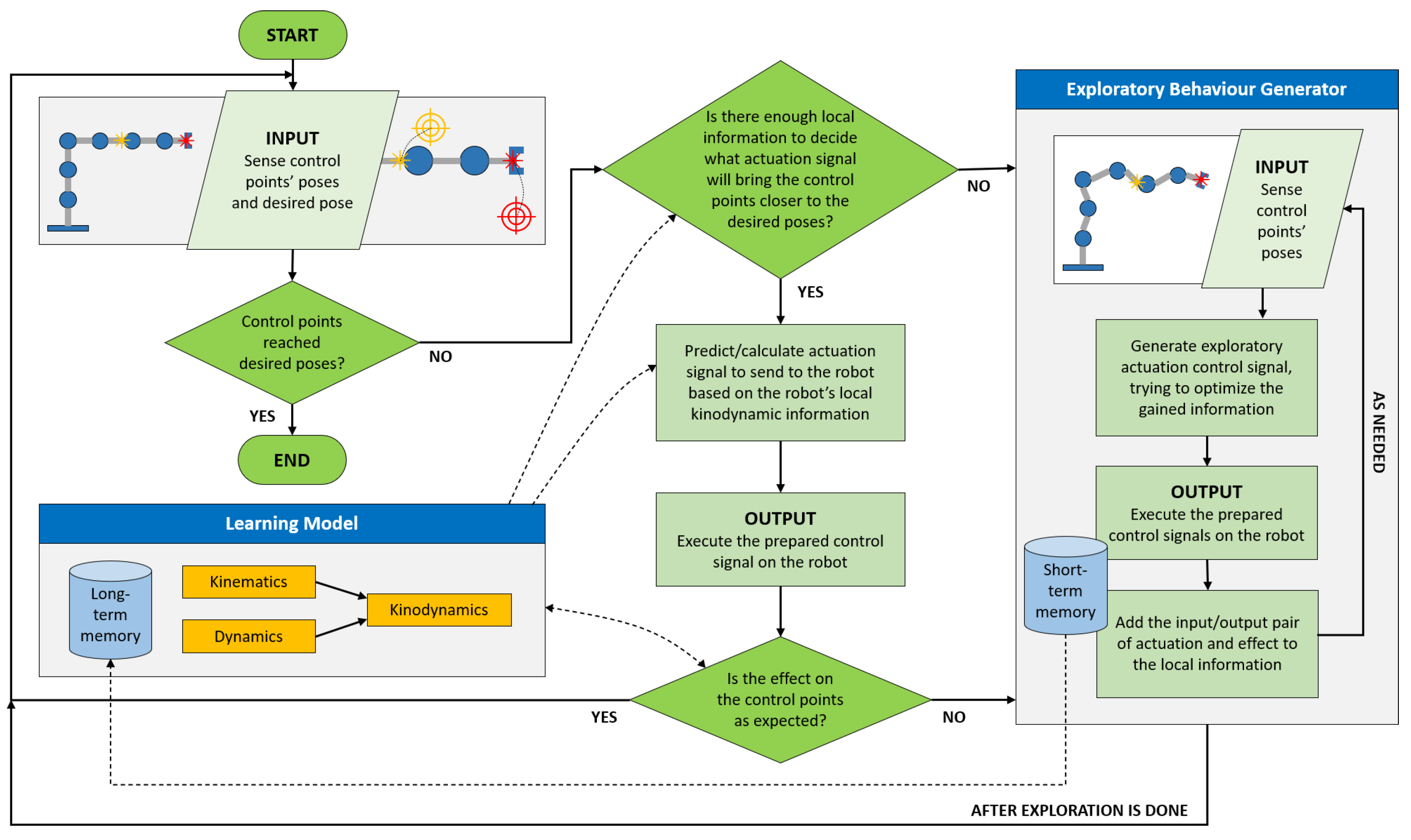
The kinematic-model-free multi-point controller, just like any other kinematic-model-free controller, assumes that the local kinodynamics information of the manipulator is attainable. This information is attained by generating pseudo-random actuation signals to actuate the robot joints and observing their result on the robot’s control point(s). A high-level diagram summarizing the kinematic-model-free multi-point approach is shown in Figure 1.

The actuation primitives produce signals $\tau \left(t\right)$ which are sent to each of the robot’s actuators and are defined as:

$$\tau \left(t\right)=\left\{\begin{array}{cc}{\tau }_p\hfill & t\in [t_0,t_0+\frac{d_p}{2})\hfill \\ -{\tau }_p\hfill & t\in [t_0+\frac{d_p}{2},t_0+d_p]\hfill \\ 0\hfill & \mathrm{otherwise}\hfill \end{array}.\right.$$

(18)

Note that actuation primitives could be motor torques, motor currents, joint positions, etc. The controller tracks the poses of the control points, ${\widehat{\mathbf{q}}}_i$, using dual quaternion representation which yield the controlled points vector:

$$\widehat{\mathbf{\varphi }}=[{\widehat{\mathbf{q}}}_i,\cdots ,{\widehat{\mathbf{q}}}_n].$$

(19)

The controller attempts to bring the points ${\widehat{\mathbf{q}}}_i$ towards desired target poses ${\widehat{\mathbf{d}}}_i^f$, yielding the desired poses vector as follows:

$$\widehat{\mathbf{\gamma }}=[{\widehat{\mathbf{d}}}_i^f,\cdots ,{\widehat{\mathbf{d}}}_n^f].$$

(20)

By controlling multiple points, redundancies can be easily resolved by specifying the desired poses of other points along the robot’s serial chain. The controller terminates when $\widehat{\mathbf{\varphi }}=\widehat{\mathbf{\gamma }}$, i.e., when the poses of the controlled points of interest coincide with their corresponding desired poses. This condition can be relaxed by allow the controlled points’ poses to reach within some deviation $\sigma$ of their respective desired target poses. Otherwise, the controller is to actuate the control points towards a set of intermediate poses ${\widehat{\mathbf{d}}}_i^t$ that lead to the final desired target poses ${\widehat{\mathbf{d}}}_i^f$ in discrete steps. The intermediate poses are found using screw linear interpolation interpolation between the current poses of the controlled points, ${\widehat{\mathbf{q}}}_i$, and desired target poses, ${\widehat{\mathbf{d}}}_i^f$. At each step, the kinematic-model-free multi-point controller estimates actuation primitives, $b_i$, to move each controlled point $i\in \mathbb{I}$ towards their respective desired poses:

$$b_i=\left[\begin{array}{c}{\tau }_p^1\left(\widehat{p}\right)\\ {\tau }_p^2\left(\widehat{p}\right)\\ ⋮\\ {\tau }_p^m\left(\widehat{p}\right)\end{array}\right],$$

(21)

where ${\tau }_p^j\left(\widehat{p}\right)$ is the magnitude of the actuation primitive of actuator j. After each step where the robot joints have been actuated, the displacement of the control points are recorded as observations, which are calculated using the $DQrel$ function. The nearest k observation dual quaternions to each point $i\in \mathbb{I}$ form the observation matrix:

$$\widehat{\mathbf{\psi }}=\left[\begin{array}{c}{\widehat{\mathbf{\psi }}}_1\\ {\widehat{\mathbf{\psi }}}_2\\ ⋮\\ {\widehat{\mathbf{\psi }}}_n\end{array}\right]=\left[\begin{array}{cccc}{\widehat{\mathbf{o}}}_1^1& {\widehat{\mathbf{o}}}_2^1& \dots & {\widehat{\mathbf{o}}}_k^1\\ {\widehat{\mathbf{o}}}_1^2& {\widehat{\mathbf{o}}}_2^2& \dots & {\widehat{\mathbf{o}}}_k^2\\ ⋮& ⋮& \ddots & ⋮\\ {\widehat{\mathbf{o}}}_1^n& {\widehat{\mathbf{o}}}_2^n& \dots & {\widehat{\mathbf{o}}}_k^n\end{array}\right],$$

(22)

where ${\widehat{\mathbf{o}}}_k^i$ is the $k^{th}$ closest observation dual quaternion of controlled point i. The actuation primitives corresponding to these observations form the actuation matrix:

$$A_i=\left[\begin{array}{cccc}{\tau }_p^1\left(p_1\right)& {\tau }_p^1\left(p_2\right)& \cdots & {\tau }_p^1\left(p_k\right)\\ {\tau }_p^2\left(p_1\right)& {\tau }_p^2\left(p_2\right)& \dots & {\tau }_p^2\left(p_k\right)\\ ⋮& ⋮& \ddots & ⋮\\ {\tau }_p^{a_i}\left(p_1\right)& {\tau }_p^{a_i}\left(p_2\right)& \cdots & {\tau }_p^{a_i}\left(p_k\right)\end{array}\right].$$

(23)

The desired actuation primitives, $b_i$, is assumed to be a linear combination of the k nearest actuation primitives such that:

$$A_i{w}_i=b_i,$$

(24)

where $w_i={[w_1^i,w_2^i,\dots ,w_k^i]}^T$ is a set of unknown weights. The weights are estimated by minimizing the following:

$$DQreg({\widehat{\mathbf{d}}}_i^t,{\widehat{\mathbf{\psi }}}_i)=\underset{w_i}{min}DQdist({\widehat{\mathbf{d}}}_i^t,DQLC({\widehat{\mathbf{\psi }}}_i,w_i)).$$

(25)

With the weights for each control point, the desired actuation is then computed using Equation (24) for each control point. The respective actuation matrix is used in the calculation. After the primitive for each control point has been obtained, the following averaging is done to dampen and stir the actuation of joints that contribute to the displacement of the control points:

$$b_i^{\prime }=\frac{{\sum }_{r=1}^{r=i}{\eta }_r^{i}Z\left(b_r\right)}{{\sum }_{r=1}^{r=i}{\eta }_r^i},$$

(26)

where the operator Z adds zero padding to a vector to keep the length equal to m, and the averaging weights matrix is a lower triangular matrix:

$$H=\left[\begin{array}{cccccc}{\eta }_1^1& 0& 0& 0& \cdots & 0\\ {\eta }_1^2& {\eta }_2^2& 0& 0& \cdots & 0\\ {\eta }_1^3& {\eta }_2^3& {\eta }_3^3& 0& \cdots & 0\\ ⋮& ⋮& ⋮& ⋮& \ddots & ⋮\\ {\eta }_1^n& {\eta }_2^n& {\eta }_3^n& {\eta }_4^n& \ddots & {\eta }_n^n\end{array}\right].$$

(27)

In the case that the averaging weights for each control point is normalized, Equation (26) would simply be:

$$b_i^{\prime }=\sum _{r=1}^{r=i}{\eta }_i^{r}Z\left(b_r\right).$$

(28)

Alternatively, to reduce the number of optimizations required, it is possible to fuse the optimization of each control point together into a wholesome expression as follows:

$$DQreg(\widehat{\mathbf{\gamma }},\widehat{\mathbf{\psi }})=\underset{w}{min}\sum _{i=1}^{i=n}DQdist({\widehat{\mathbf{d}}}_i^t,DQLC({\widehat{\mathbf{\psi }}}_i,w)),$$

(29)

where the weights are later used in $A_{n}w=b$ to estimate the required actuation. After each discrete actuation, the resulting displacement on the pose of each control point is compared to the expected displacement. Should the difference be significant, a new exploratory phase is triggered to collect more data about the robot’s local kinodynamics as shown in Figure 1. The controller leaves the exploratory phase once it has completed a predefined number of exploratory steps. The controller terminates once all control point poses have reached the desired poses or close enough to them, $DQdist(\widehat{\mathbf{q}},\widehat{\mathbf{d}})<\sigma$.

This controller, just like its other kinematic-model-free predecessors, does not require any prior model of the robot’s kinodynamics. As such, the controller is agnostic to any kinodynamic changes in the robot, such as alteration in the robot’s link dimensions. Since the kinematic-model-free multi-point controller is not based on any accurate robot model, the accuracy of the controller is less than conventional controllers. Moreover, this controller operates in discrete steps, making it significantly slower than other controllers and the motion can be relatively jerky. As with other complex models, such as those found in References [26,27], it is difficult to proof the convergence of the kinematic-model-free controller due to the nonlinear functions that are involved.

5. Simulation Results

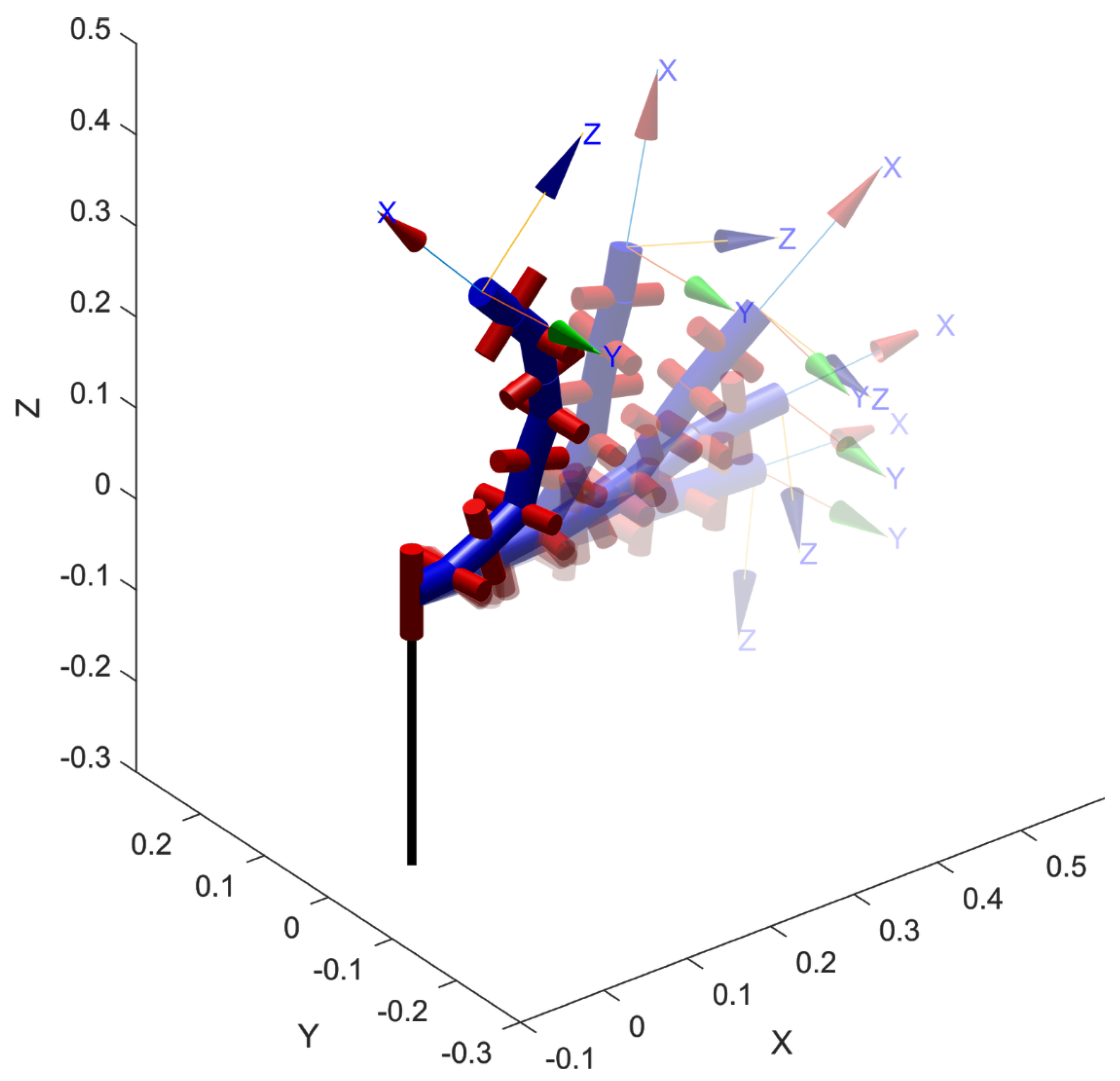
The controller is tested on a simulated redundant 9-degrees-of-freedom continuum robot, shown in Figure 2.

The robot was simulated using Matlab’s Robotics Toolbox [28] and DQ Robotics Toolbox [29]. The actuation primitives used were joint position command signals to drive the control points towards the target poses. The Denavit–Hartenberg parameters of the robot is listed in

Table 1. Denavit–Hartenberg parameters of redundant robot.

Link	${\mathit{d}}_{\mathit{i}}$	${\mathit{\theta }}_{\mathit{i}}$	${\mathit{a}}_{\mathit{i}}$	${\mathit{\alpha }}_{\mathit{i}}$
1	0	0	0.05	1.5708
2	0	0	0.05	1.5708
3	0	0	0.05	−1.5708
4	0	0	0.05	1.5708
5	0	0	0.05	−1.5708
6	0	0	0.05	1.5708
7	0	0	0.05	−1.5708
8	0	0	0.05	1.5708
9	0	0	0.05	0

.

The controller was programmed as described in Section 4 using $k=4$ nearest neighbors that comprise of actuation primitive and observation pairs. Since the experiments were conducted in simulation, a tracking camera was not needed to determine the poses of the control points. In addition, actuators discovery was also omitted in the simulation. Instead, the simulator provided these information directly. Furthermore, gravity was omitted in the simulation to keep the focus on multi-point pose control, deferring gravity compensation to future work.

Three experiments were performed to study the capabilities of the proposed kinematic-model-free multi-point controller. The first experiment involved end-effector pose control for the continuum robot with increasing number of degrees of freedom enabled. This experiment shows the degrading performance of the controller when increasing the number of degrees of freedom using a single control point. In the second experiment, the 9-degrees-of-freedom continuum robot was controlled using 1, 2, and 3 control point(s). This experiment highlights the capability of the kinematic-model-free multi-point controller to control robots of high degrees of freedom and resolve redundancies. Lastly, the robustness of the kinematic-model-free multi-point controller was measured by executing the simulation experiment 100 times with randomly-generated configurations.

5.1. Single-Point Control

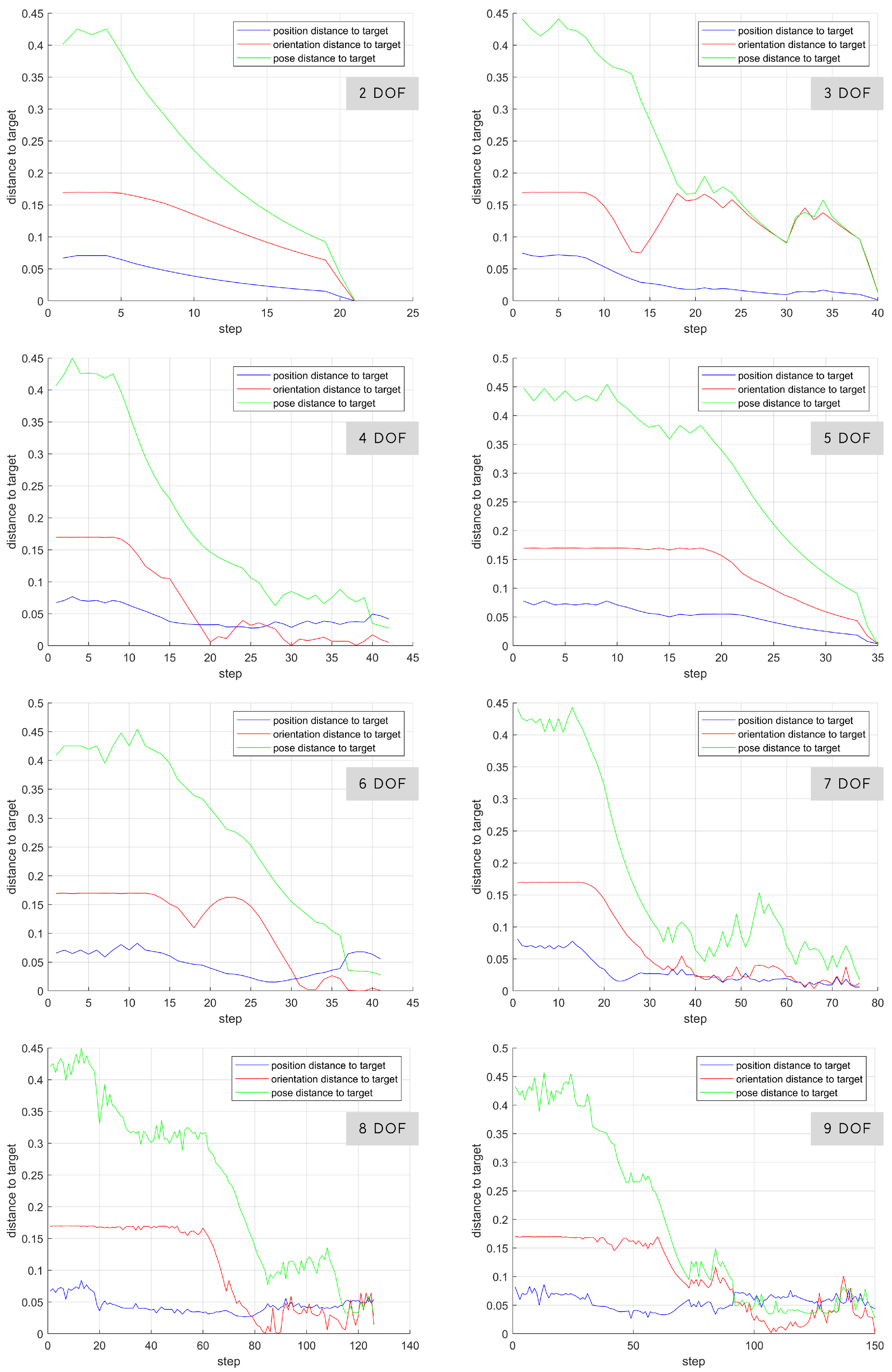
In the first experiment, a single control point situated at the end effector of the continuum robot was used to actuate the robot towards a desired target pose. Initially, only the last 2 joints of the robot were enabled. Gradually, an extra joint was enabled, increasing the robot’s degrees of freedom. The robot began from the home pose where the control-point’s task-space position was (0, 0, 0.4500), and orientation was (0, 0, 3.1416). Orientations in this paper are specified in ZYX Euler angle representation for simplicity. The target position was (0.4218, 0.0240, 0.0605) and orientation was (0.6202, −0.6009, 2.7578). The results are shown in Figure 3 and tabulated in

Table 2. Reaching steps for different degrees of freedom enabled.

Degrees of Freedom	Steps to Reach
2	21 steps
3	40 steps
4	42 steps
5	35 steps
6	41 steps
7	76 steps
8	127 steps
9	150 steps

.

In the simple 2-degrees-of-freedom case, the control point converged to the target pose within 25 steps. When increasing the degrees of freedom, it is noted that the controller takes longer to converge. Although it is evidently possible to reach the target pose within 25 steps, the added redundancies introduced additional nonlinearities that require excessive exploratory behavior. In the case where all 9 joints of the robot were enabled, the control point reached the target pose in 150 steps, a significant decrease in performance. With the stopping condition ($DQdist<\sigma$) applied, it can be seen that the controller can terminate before fully reaching the target pose.

5.2. Multi-Point Control

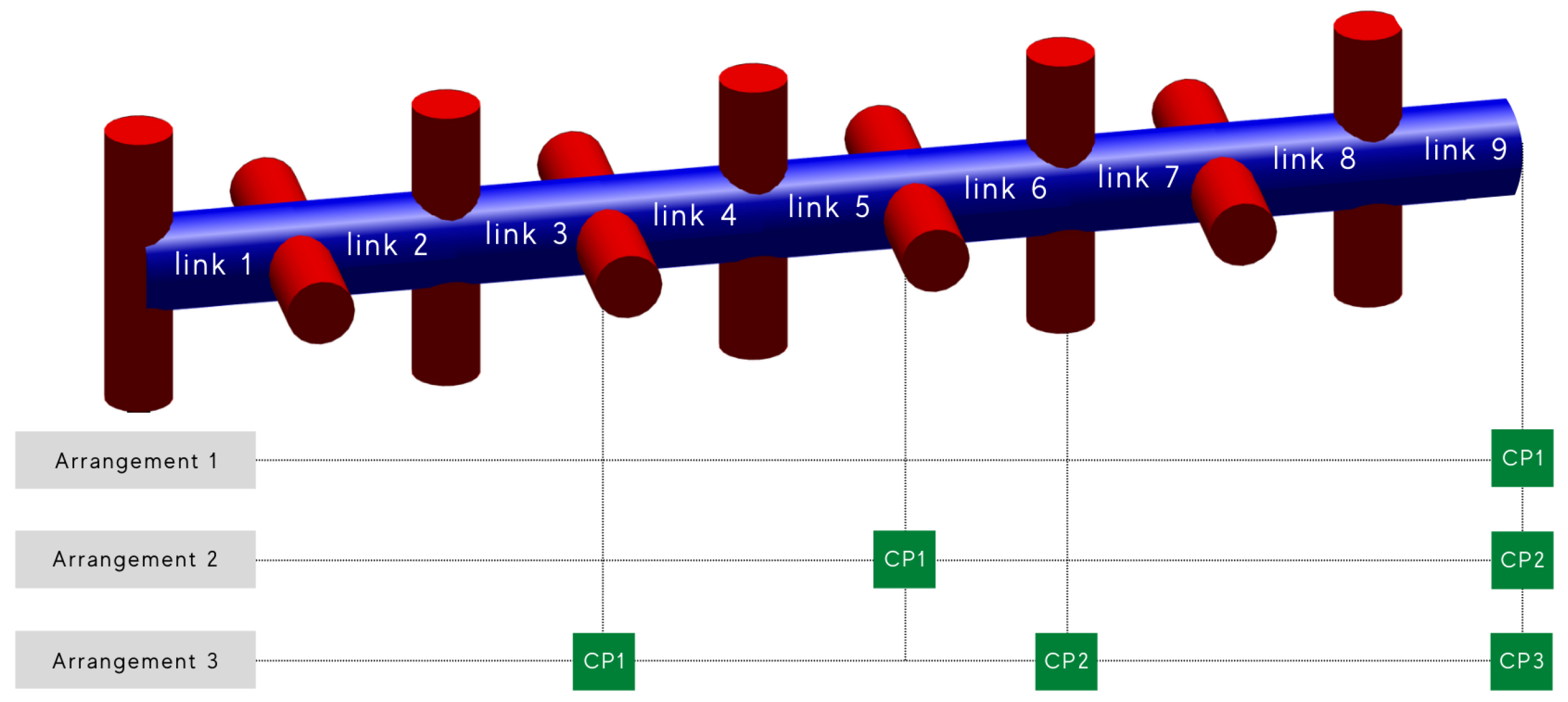
In this experiment, multiple control points were added to the continuum robot. In the first arrangement, only a single control point was added that was situated at the end effector. In the second arrangement, 2 control points were added, one at the end effector and one at the end of link 5. Finally, in the third arrangement, the 3 control points were added that were evenly distributed throughout the robot’s kinematic chain. The placements of the control point for each arrangement are summarized in

Table 3. Control points placement.

Arrangement	Control Point 1	Control Point 2	Control Point 3
1	end effector	-	-
2	end of link 5	end effector	-
3	end of link 3	end of link 6	end effector

.

These arrangements are depicted in Figure 4. Three reaching tasks were preformed with each arrangement. All desired poses were within the robot’s configuration space. See Figure 5. The reaching tasks increased in complexity in terms of dexterity required. We note that arrangement 1 corresponds to kinematic-model-free control of the end-effector pose. Thus, this experiment also serves as a comparison with the kinematic-model-free orientation controller in Reference [5]. The results are shown in Figure 6 and tabulated in

Table 4. Steps required to complete three reaching tasks using three arrangements of control points.

Task		Arrangement
	1	2	3
1	70 steps	64 steps	46 steps
2	93 steps	59 steps	35 steps
3	185 steps	147 steps	92 steps

.

Only the pose distance of the control point situated at the end effector is shown. It can be seen that the controller converges faster to the desired pose when using more control points situated along the robot’s kinematic chain. In task 1, we note that a 66% improvement in convergence speed when using 3 control points. In task 2 and 3, there was a 38% and 50% improvement was measured, respectively. These results indicate that adding more control points will improve convergence and resolve redundancies in hyper-redundant systems. As for accuracy, the termination criteria was set to DQdist < 0.03, achieving a close enough reaching accuracy.

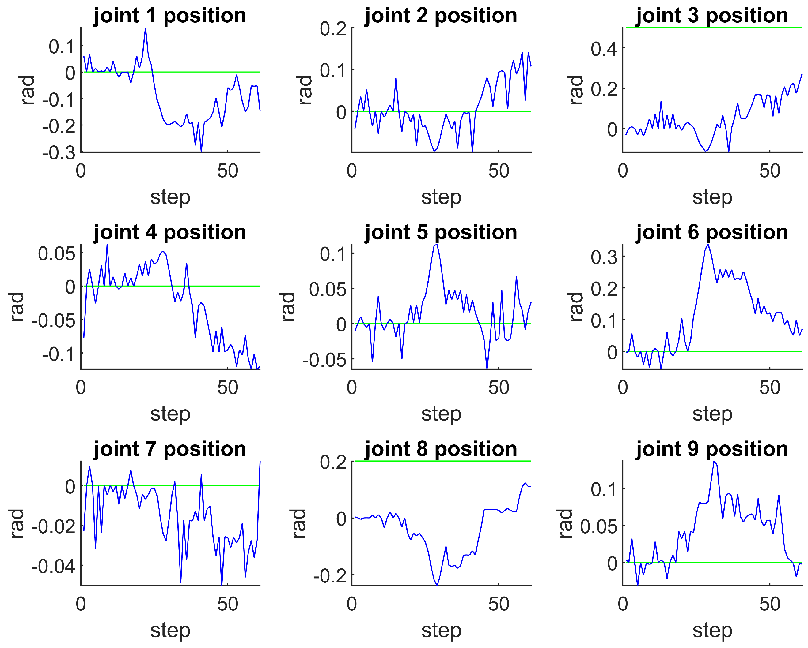
Furthermore, to demonstrate the joints’ position during an execution, the joint position are shown in Figure 7. The larger jitters in joint positions correspond to exploratory behavior, which is triggered whenever there is deficiency in local kinodynamic information.

5.3. Robustness

The robustness of the algorithm was measured by executing the simulation 100 times. Each time, the robot must reach a randomly-generated pose that is within its configuration space and it reachable within 150 steps. If the controller takes longer, the simulation is restarted. Three control points were used. One interesting configuration is shown in Figure 8. The controller managed to achieve this bent arch configuration within 150 steps.

It was observed that 82% of the runs, the controller manages to reach to the target pose. However, in 18% of the runs, the controller did not successfully converge to the solutions that brought the robot’s end effector to the desired poses. This can occur when the optimization is stuck in a local minimum, which results in an inaccurate actuation signal that does not optimally move the control points towards the target poses.

6. Conclusions

This paper presents a novel kinematic-model-free control for controlling the pose of multiple points along the kinematic chain of a continuum robot. The proposed controller is able to resolve redundancies and converge faster to a desired configuration. The controller works by actuating the robot using randomly-generated actuation primitives and observing their effects on the control points. This information is then used to build a local linear model using locally weighted dual quaternions. The local linear model is then used to calculate an actuation primitive and actuate the continuum robot towards a desired pose.

In the first experiment, it was evident that the performance of the controller worsened in terms of convergence when increasing the degrees of freedom of the robot. The higher the degrees of freedom, the longer it took to converge. This is due to the nonlinearities introduced, making the local linear model less accurate.

We presented the generalized kinematic-model-free multi-point controller and the method by which observations are used to calculate actuation primitives that will reduce the distance between a robot’s current pose and its desired target pose. The simulation results in the second experiment show that this novel controller is capable of performing reaching tasks without any prior kinematic model of the robot, successfully actuating the poses of the control points towards some desired configuration.

Three arrangements for the control points were tested on a simulated 9-degrees-of-freedom continuum robot. Three different robot configurations were targeted, all of which are within the robot’s configuration space. It was noted that, when more control points were used, the controller performed better and converged faster to the desired target robot pose. Controlling multiple points along a robot did not only resolves redundancies, but proved to converge faster to the desired pose.

Finally, the controller’s robustness was tested by executing the simulation 100 times using random target configurations which the controller had to reach. The random target configurations lied within the robot’s configuration space. The kinematic-model-free multi-point controller succeeded in reaching the target poses within 150 steps 82% of the times.

The proposed controller can be used in applications where simultaneous translational and rotational reaching of redundant robots is required. The controller is useful for resolving redundancies of continuum robots. The kinematic-model-free approach in general can be used for new robots where a model is not readily-available or for robots that are hard to model. In general, the controller is applicable where flexibility is favored over precision and speed. Examples of such applications include use of soft robots for reaching, drawing, picking-and-placing, etc. As for future work, continuous control, gravity compensation, joint limits, joint friction, and physical implementations, are promising research directions to be investigated. These challenges must be addressed before deploying the kinematic-model-free controller on any physical system.