Development and Evaluation of the Traction Characteristics of a Crawler EOD Robot

Abstract

Today, terrestrial robots are used in a multitude of fields and for performing multiple missions. This paper introduces the novel development of a family of crawling terrestrial robots capable of changing very quickly depending on the missions they have to perform. The principle of novelty is the use of a load-bearing platform consisting of two independent propulsion systems. The operational platform, which handles the actual mission, is attached (plug and play) between the two crawler propulsion systems. The source of inspiration is the fact that there are a multitude of intervention robots in emergency situations, each independent of the other. In addition to these costs, there are also problems with the specialization of a very large number of staff. The present study focused on the realization of a simplified, modular model of the kinematics and dynamics of the crawler robot, so that it can be easily integrated, by adding or removing the calculation modules, into the software used. The designed model was integrated on a company controller, which allowed us to compare the results obtained by simulation with those obtained experimentally. We appreciate that the analyzed Explosive Ordnance Disposal (EOD) robot solution represents a premise for the development of a family of EOD robots that use the same carrier platform and to which a multitude of operational platforms should be attached, depending on the missions to be performed.

1. Introduction

The most serious threat to the civilized world, following nuclear threats, is terrorist threats [1]. In recent decades, due to the expansion of civilization across the globe, and the ease of access to information, technology and culture, extremist actions and reactions have proliferated [2]. They are symmetrical with extremism in the process of globalization and aim to stop and destabilize the offensive growth of the civilized world against increased fragmentation, promiscuity, poverty and violence [3].

Terrorism does not have a generally accepted definition. The difficulty of defining it stems both from its complexity and from a wide divergence of positions of individuals, organizations or states involved in the fight against terrorism [4]. The simplest definition is “purpose and method”: Terrorism is an unconventional fighting tactic used to achieve strictly political goals that are based on acts of violence, sabotage or threat, executed against a state, organizations, social groups or against a group of civilians, with the precise purpose of producing a generalized psychological effect of fear and intimidation [5]. The ultimate goal is to put pressure on that entity to get it to act in accordance with the wishes of the terrorists if that goal cannot be achieved by conventional means [6].

The correct and complete definition and understanding of the phenomenon of terrorism are absolutely necessary for the elaboration of effective strategies and tactics in the fight against it [7]. As there is no valid general model, the definition and analysis of the terrorist act must be done on a case-by-case basis. The main defining elements of terrorism [8] are: Means: violent actions [9]; Method: inducing fear for citizens [10]; Target: civilians (non-combatants) [11]; Purpose: to bring about a major political change [12]; Actors: individuals or non-state groups [13].

On the other hand, terrorism uses only one type of action—surprise attacks of small magnitude but of maximum intensity on people, infrastructures and institutions. The procedures for such attacks are endless [14]. Among the most common terrorist acts, we mention: surprise attack with firearms; bomb attack; attack of infrastructures of any kind (sophisticated artisanal systems) [15]; attack on public places and public institutions [16]; radiological attack [17]; chemical attack [18]; biological attack [19].

There are, of course, many other forms of terrorist acts. Therefore, the main forms and procedures of counter-terrorism actions must respond promptly to these challenges, and must be anticipatory, preventive, effective and dissuasive [20].

In previous studies, no specific forms and procedures in the war on terrorism have been found, but actions and measures have been initiated by all structures, forces and institutions to protect themselves against terrorist attacks. That is why we followed the description, quite exhaustively, of the testing procedures, which allows for the validation of the developed analytical–numerical model.

In this stage of project development, the formulation of research hypotheses for our model refers to the validation of the analytical–numerical model regarding the ability of the robot to move in different environments (structured/unstructured), the validation being experimentally performed. The solution proposed in the article has already been implemented, and the obtained results encourage us to move towards the development of operational platforms with multi-role destinations. The software architecture is modular, and the proposed algorithm can be upgraded relatively easily, by simply inserting or removing modules. Additionally, the proposed mechanism can provide a basis for discussion/development for those interested in developing EOD robots. On this basis, the results showed that the robot can operate on an operational platform specific to the actions of taking over and relocating objects that are considered to be suspicious.

Regarding the novelty of the project, we consider that the possibility to assemble an intervention robot at the crime scene, according to the identified specific, is much more useful than more expensive and complex logistics. On top of that, the price of the prototype robot (designed and made) is 1/10 compared to a similar robot in the same class, respectively compared to TELEROB (https://www.telerob.com/de/ (accessed on 18 February 2021)); most robots in the same class are made to perform a single mission, it is a robot that at the maximum opening of the arm can support 15 kg, even when there is no power supply. This could be achieved by introducing electromagnetic brakes in each joint from R0 to R5; with the available resources we were able to make a multifunctional robot, only by changing the operational platform, given that the design and assembly were performed entirely in ATM, only the mechanical elements were made at the industrial partner.

The paper is structured as follows: Section 2 highlights the state of the art in the field of EOD; Section 3 shows how the geometric configuration of the crawler robot was established; Section 4 details the performance of simulations based on the defined analytical–numerical model; Section 5 details the evaluation tests of the propulsion system in order to validate the analytical–numerical model; Section 6 presents the conclusions.

2. State of the Art

Currently, mobile robotics is at the intersection of several fields of science. These systems include: Knowledge representation [21]: the field of artificial intelligence helps to obtain an internal model of the world associated with the task performed by the robot, and uses data structures and specific algorithms to represent the characteristics of objects in the environment; Natural language [22]: natural language changes quite frequently, so simple word recognition is no longer enough to understand the real meaning of a processed text; Learning [23]: ideally, a robot could learn the tasks it has to perform by simply repeating similar actions performed by a human operator; Planning and problem solving [24]: intelligence is inherently associated with the ability to plan actions needed to achieve a particular goal, as well as the ability to solve problems that arise when these action plans do not work; Inference [25]: by inference, it is possible to fill in the missing information to solve a certain problem; Search [26]: in terms of artificial intelligence, search means the efficient examination of a representation of knowledge, specific to a certain problem (search in a “space”) in order to determine a solution; Vision [27]: by creating artificial vision systems, the actions of the mobile robot can be made more precise and complex. Sometimes, mobile robots appear in the form of vehicles capable of operating autonomously on the ground (UGVs—Unmanned Ground Vehicles), in the air (UAVs—Unmanned Aerial Vehicles) or in the water (UUVs—Unmanned Undersea Vehicles). In the broadest sense of the definition, a mobile robot is a real-time integrated system (embedded real-time system), that has sensors [28] for environmental perception, execution elements for performing actions on the environment and a control system for mapping perception in action [29]. Perception and action are the major aspects that define a mobile robot. Depending on the organization of these three functional aspects, it can be considered that the mobile robot has a greater or lesser degree of autonomy.

The best-known type of mobile robot is the Automated Guided Vehicle (AGV—Automated Guided Vehicle). AGVs operate in pre-programmed environments and are inflexible and “fragile” in operation; thus, any unforeseen route changes (objects on the runway) can lead to a compromise of the entire mission [30].

The alternative to AGV is to build mobile robots with autonomy in motion to travel in the environment to perform various tasks; adapt to changes in the environment; learn from experience and change their behavior accordingly (how to act); build internal representations of the world around them that can be used for decision-making processes (for example, for navigation).

These characteristics allow for the use of these robotic structures in specific applications (Figure 1): transport operations, exploration, surveillance, orientation, inspection, evolution in environments inaccessible or hostile to the human operator such as robots intended to combat terrorist actions, or robots operating in contaminated environments, underwater robots, planetary exploration vehicles, etc. [31].

2.1. The Functions of a Crawler Mobile Robot

From a functional point of view, a mobile robot consists of three modules: the role of the sensor module is to estimate the speed and position of the mobile robot [32,33,34]; the orientation module is the reference generator for the orientation of the mobile robot in space [33]; the control module is the subsystem that generates the control quantities for the execution elements based on the data provided by the orientation module [34].

The following essential functions of a mobile robot can be defined according to the functional modules:

A.

Navigation function [35]: workspace representation; avoidance of obstacles; location function; motion planning; motion control.

B.

Task Planning Function [36]:

C.

Interaction and communication function [37].

2.2. Justification for the Use of a Crawler Mobile Robot for EOD Actions

Anti-terrorism intervention requires the use of robots to limit risks for the following reasons: performing procedures during IED intervention missions, which include observation and inspection, X-ray analysis, disruption, etc.; no matter how careful the operator is in responding to the IED, there is always the possibility that the attacker may be nearby so that he can operate the explosion-proof device remotely; even if a robot cannot neutralize an IED, it can still be used to provide information on the choice of procedure and devices needed to evacuate/eliminate the dangerous object from the threatened area.

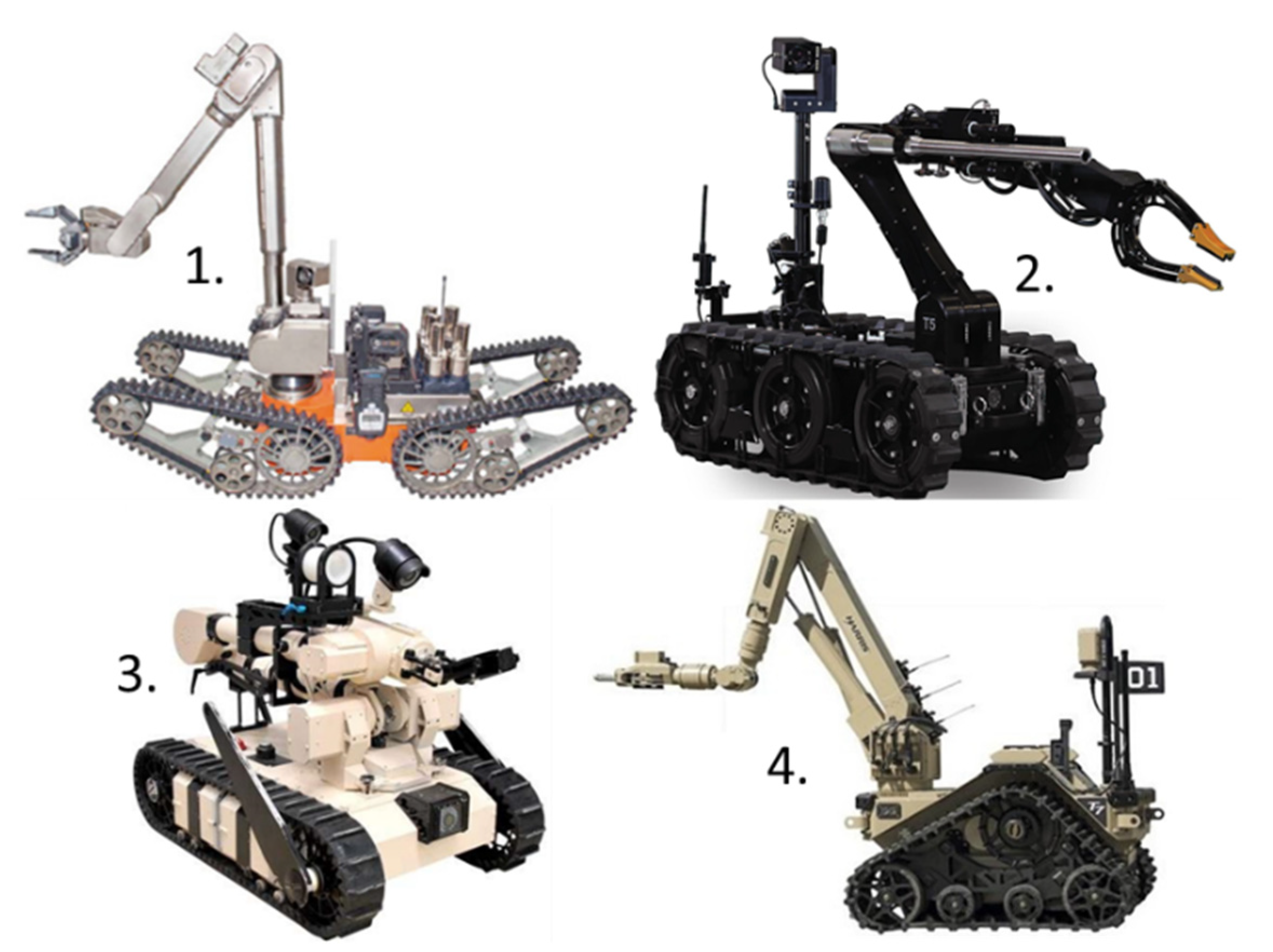
2.3. Features of Crawler Mobile Robots

Named mobile robots and controlled/autonomous vehicles, robot trailers or robotics, have a structure consisting of (Figure 2):

Mobile intervention robots have the following main features: degree of mobility: following a varied trajectory in terms of shape, length, and number of parking/stopping points [44]; speed: it is between 1–10 m/s, depending on the environment in which it moves inside/outside [45]; autonomy: is the dependence on own power sources or the length of the power cord [46]; remote control and automation of operations [47].

2.4. Requirements for Crawler Mobile Robots, Resulting from an Anonymized Market Study

The robot should be affordable, if the designers meet the following requirements, simultaneously or individually: is intended only for specific missions and threats, for example pyrotechnic intervention [48]; is built modularly [49]; subsystems to be redesigned so that the solution is as simple and reliable as possible [50]; can use a disruptor [51]; should be equipped with video cameras [52]; must have an adequate lifting capacity [53]; can use X-ray systems [54]; should be equipped with omnidirectional cameras [55]; the robot must be able to communicate with an operator [56]; can easily climb stairs it can be said that only 10% of the threats targeted easily accessible open areas; should be easy to maintain and repair; must operate in a wide range of terrains [57]; arm should have high mobility [58].

3. Geometric Configuration of the Crawler Propeller

In order to achieve the geometric configuration of the crawler engine, one must consider the influence of the geometric characteristics of the tracked engine on the following: mobility of the robot on terrain with various configurations and consistencies; stability of the robot during movement and during the execution of the specific mission. The effects of the terrain on the robot can be grouped into the categories presented in Figure 3.

Analyzing the requirements formulated by the potential beneficiaries, as well as the current stage of technological development of mobile robots, the main functional parameters were quantified, and the main functional characteristics were estimated (

Table 1. Type-dimensional and actuation requirements for the EOD robot under analysis.

Characteristics	U.M.	Amount
Fully equipped mobile robot table	kg	250
Maximum speed on horizontal terrain	m/s	1
Maximum slope when walking straight	deg	30
The height of the steps	mm	150
Average ground pressure	MPa	0.05
The height of the stepped obstacle crossed	mm	225
The width of the ditch crossed	mm	800
Depth of water on hard horizontal ground	mm	100
Race of turns	mm	continuously variable
Minimum turning radius	mm	0–rotation
Travel control	-	wireless
The mass of the manipulated object	kg	25
Range of the manipulator arm	mm	1000
Rotate the manipulator arm to the side	deg	30
The gripping length of the gripping mechanism	mm	150
Arm displacement position	-	folded/extended
Omnidirectional video camera for travel	buc.	2
Video camera for inspection	buc.	2
Riding the platform while working	-	no
Working autonomy	h	6
Construction type	-	modular

).

The global analysis of the problem of locomotion on surfaces leads to the identification of four types of forces, among them including the propulsive force: Propulsion; Adhesion; Cohesion; Support.

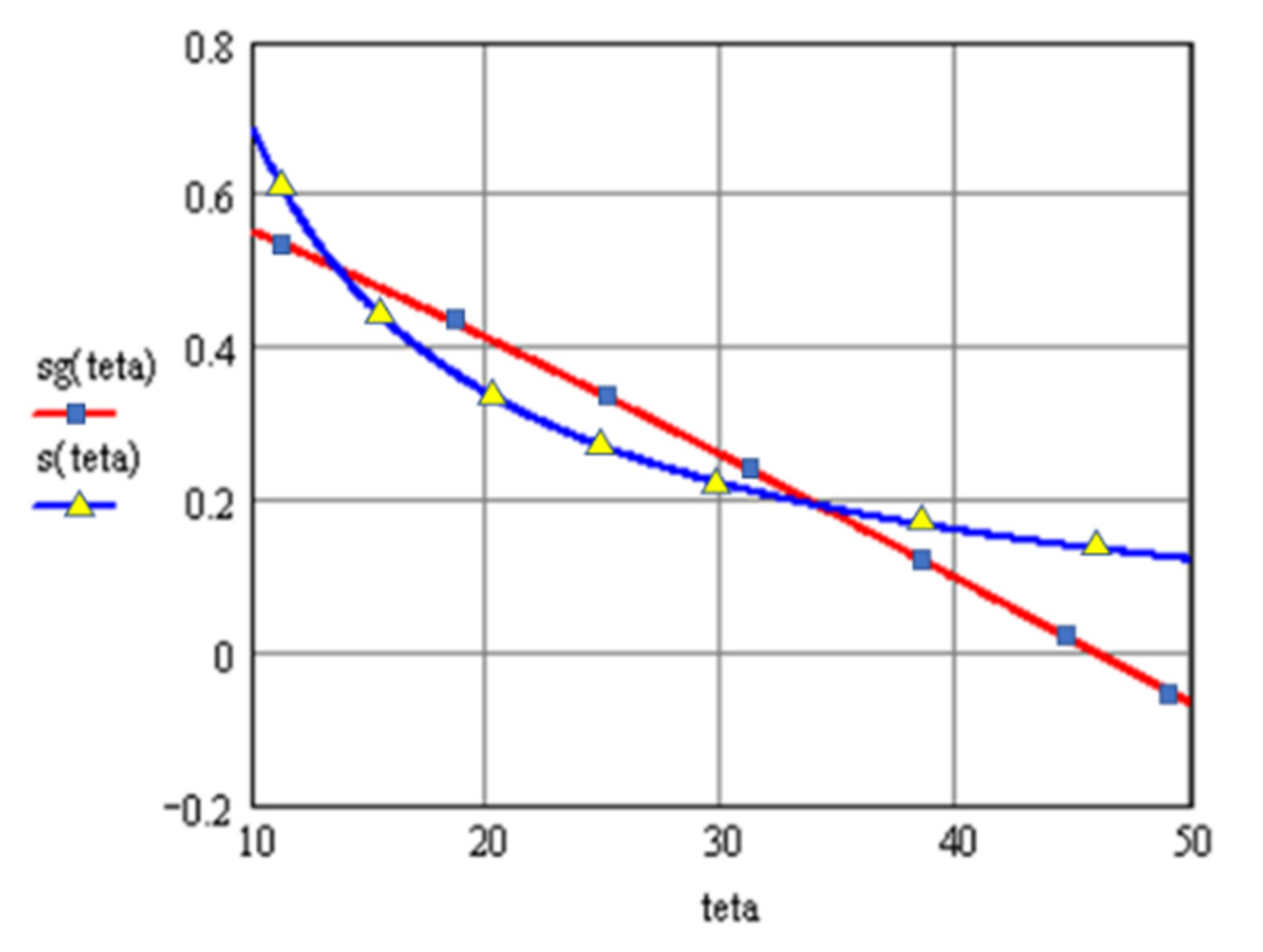
3.1. Conditions Regarding the Crossing of the Step Type Obstacle

The step type obstacle is often encountered in urban environments (curbs, stairs in buildings, etc.), which requires a detailed study of this process for an optimal geometric configuration of the crawler engine (Figure 4). The crossing of the step-type obstacle presupposes the obligatory completion of two successive stages: the approach to the obstacle; crossing the obstacle.

The ascending force arises T_asc [N]. Its value is limited by: φ_t [−] and φ_obs [−].

$$T_t={\mathsf{\phi }}_t\cdot G \left[N\right],$$

(1)

where: $T_t\left[N\right]$—traction force, manifested at the wheel; $G\left[N\right]$—the weight of the robot.

The ascending force is given by the following relation:

$$T_{asc}={\mathsf{\phi }}_{obs}\cdot Z={\mathsf{\phi }}_{obs}\cdot T_t={\mathsf{\phi }}_{obs}\cdot {\mathsf{\phi }}_t\cdot G \left[N\right],$$

(2)

where: $T_{asc}\left[N\right]$—the ascending force, manifested in front of the tensioning roller, at the contact of the track with the obstacle.

The limiting condition for them of climbing the obstacle is:

$$T_{asc}(L_a+l_a)=G\cdot x_G \left[N\right],$$

(3)

$${\mathsf{\phi }}_{obs}{\mathsf{\phi }}_t\ge \frac{x_G}{L_a+l_a}\equiv {\mathsf{\phi }}_{obs}{\mathsf{\phi }}_t\ge \frac{x_G}{L},$$

(4)

where: CG—weight center; $y_G\left[m\right]$—distance from the CG to the running surface, on the axle Oy; $r_m\left[m\right]$—drive wheel radius; $r_a\left[m\right]$—the radius of the tension roller; $h_a\left[m\right]$—distance from the axis of the tension roller to the tread, on the axis Oy; ${\alpha }_a\left[\mathrm{deg}\right]$—the angle of inclination of the ascending branch of the track to the axis Ox; $x_G\left[m\right]$—distance from the CG to the axle of the drive wheel, on the axle Ox; $L_a\left[m\right]$—the distance from the axle of the drive wheel to the last roller, the one at the beginning of the ascending branch of the track, on the axis Ox; $l_a\left[m\right]$—distance from the center of the last roller to the center of the tension roller, on the axis Ox.

The coefficient of friction between the tracked thruster and the obstacle (Figure 5), μ [−], is given by the following calculation relation [60,61,62]:

$$\mathsf{\mu }\ge \frac{L-L_1}{L_1+R/\sqrt{1-{\left(\frac{h-R}{L}\right)}^2}} [-],$$

(5)

where: $h\left[m\right]$—the height of the obstacle step, on the axis Oy; $\Delta =h-h_a \left[m\right]$—the difference between the height of the step obstacle and the height of the axis of the tension roller, on the axis Oy; $L_1\left[m\right]$—the distance from the axis of the drive wheel to the CG, along the longitudinal axis of the robot; $L-L_1\left[m\right]$—the distance from the CG to the axis of the tension roller, along the longitudinal axis of the robot; $\mathsf{\beta }\left[\mathrm{deg}\right]$—the angle of inclination of the longitudinal axis of the robot with respect to the axis Ox.

Which is denoted by λ, the ratio:

$$\lambda =\frac{L_1}{L} [-],$$

(6)

Thus, (5) becomes:

$$\mathsf{\mu }\ge \frac{1-\lambda }{\lambda +R/L\sqrt{1-{\left(\frac{h-R}{L}\right)}^2}} [-],$$

(7)

In order to assess the influence of the length of grip and the position of the center of gravity, the height of the obstacle shall be considered to be: $h=1,5\cdot r_m$. It is denoted as $\gamma =r_m/L$, so that inequality (7) becomes:

$$\mathsf{\mu }(\lambda ,\gamma )\ge \frac{1-\lambda }{\lambda +\frac{2\gamma }{\sqrt{4-{\gamma }^2}}} [-],$$

(8)

The above relation allows for the evaluation of the influence that the position of the center of mass has on the conditions of escalation of the obstacle (Figure 6).

Given the notation presented in Figure 7, the following equations result:

$$s_G=r\sin \mathsf{\theta }+x_G\cos \mathsf{\theta }-y_G\sin \mathsf{\theta } \left[m\right],$$

(9)

$$h=r-r\cos \mathsf{\theta }+d\sin \mathsf{\theta } \left[m\right],$$

(10)

$$d=\frac{\left(h-r+r\cos \mathsf{\theta }\right)}{\sin \mathsf{\theta }} \left[m\right],$$

(11)

$$s=r\sin \mathsf{\theta }+d\cos \mathsf{\theta }=r\sin \mathsf{\theta }+\frac{\left(h-r+r\cos \mathsf{\theta }\right)}{\sin \mathsf{\theta }} \left[m\right],$$

(12)

where: r [m]—the running radius of the support wheel (bucket), including the thickness of the track; h [m]—the height of the step obstacle.

Analyzing the way in which the vehicle climbs onto the obstacle, the following distinct situations can be distinguished: $s_G<s$—the vehicle can climb over the obstacle; $s_G>s$—the vehicle cannot climb over the obstacle; $s_G=s$—critical condition, at the limit.

From the analysis of the Equations (9)–(12), from the graphical representation of these equations (Figure 8) and of the presented limit conditions, it results in (13):

$$r\sin \mathsf{\theta }+x_G\cos \mathsf{\theta }-y_G\sin \mathsf{\theta }=r\sin \mathsf{\theta }+\frac{\left(h-r+r\cos \mathsf{\theta }\right)\cos \mathsf{\theta }}{\sin \mathsf{\theta }} \left[m\right].$$

(13)

$$x_G\sin \mathsf{\theta }\cos \mathsf{\theta }-y_G{\sin }^2\mathsf{\theta }=\left(h-r\right)\cos \mathsf{\theta }+r{\cos }^2\mathsf{\theta } \left[m\right].$$

(14)

Solving Equations (13)–(14) was performed for a running radius of 0.0425 m (Figure 9).

How to vary the maximum angle of arrangement of the support branch of the track to the ground θ is shown in Figure 9 and Figure 10. It can be seen that the angle of inclination decreases as the center of mass moves forward.

The schematic of the tracked platform geometry for the trench crossing limit situation is presented in Figure 11. In the initial phase, the vehicle (drawn in blue) remains horizontal until the vertical passing through the center of mass coincides with the edge of the ditch. The vehicle starts to oscillate around the point of contact with the edge of the ditch (point marked with P). The limit position, at which it is still possible to cross the ditch (drawn in red) occurs when contact is made with the other edge of the ditch at a point on the circumference of the front wheel on its horizontal axis of symmetry. The above-mentioned approach scenario neglects inertial forces due to the low travel speeds of the mobile robot platform. For the limit situation, the following geometric equations can be written:

$$(L-L_1)\cos \mathsf{\phi }+h_r\sin \mathsf{\phi }+R\cos \mathsf{\phi }=L_s \left[m\right].$$

(15)

$$(L-L_1)\sin \mathsf{\phi }-h_r\cos \mathsf{\phi }+R\sin \mathsf{\phi }=0 \left[m\right].$$

(16)

for the general case, in which it was assumed that $h_r>r_m$ $h_r>r_m$.

Eliminating the unknown φ, the width of the ditch that can be crossed was calculated according to the horizontal position of the center of mass and using the notation $\gamma =L/L_1$, the results shown in Figure 12 are obtained.

There is an inversely proportional dependence between the maximum width of the ditch that can be crossed and the horizontal distance from the rear wheel axle and the center of mass. It turns out that the forward movement of the center of mass leads to an increase in the height of the step that can be climbed, but also to a decrease in the width of the ditch that can be crossed.

3.2. Conditioning Imposed by the Average Pressure on the Ground

The average pressure exerted by the tracks on the ground is given by the following relation:

$$p_{med}=\frac{G}{2\cdot b\cdot L_a} \left[\raisebox{1ex}{$N$}\!\left/ \!\raisebox{-1ex}{$m^2$}\right.\right].$$

(17)

where: b [m]—width of the track; L_a [m]—adhesion length of the track to the ground.

Using the relation (17) the “Contour Plot” type graph was obtained (Figure 13).

In Figure 13, it can be naturally concluded that the area located in the upper right, for which $p_{med}<6 \left[\mathrm{kPa}\right]$, is the most advantageous. An average–low ground pressure can be obtained by increasing the adhesion length and/or by increasing the track width.

However, reporting to military vehicles is not able to generate consistent values for the recommended average ground pressure due to the “scale effect” [62,63] (Figure 14).

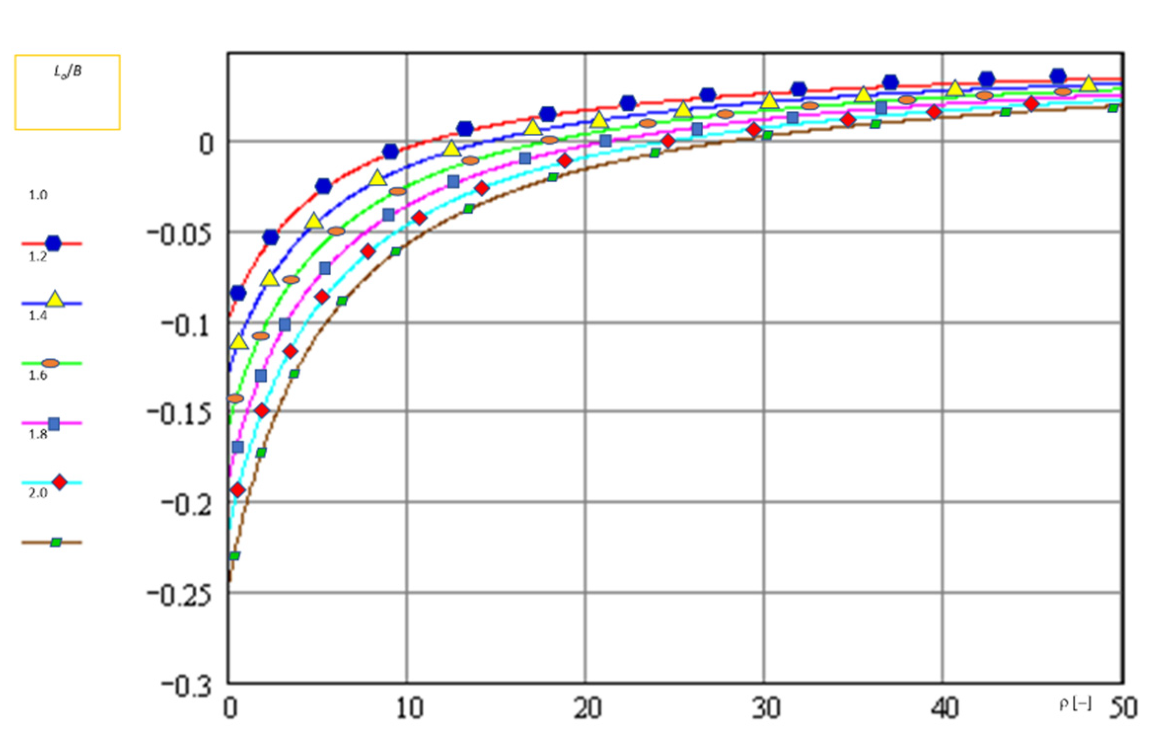
3.3. Geometric Conditions Imposed by the Execution of the Turn

From the point of view of cornering, there are two major conditioning factors: the position of the center of mass and the gauge (the distance between the planes of symmetry of the two tracks).

The position of the center of mass (CG) directly conditions the distribution of the pressure exerted by the support branch of the track on the ground. The value of the displacement of the turning poles is obtained by solving the following equation [64]:

$$\frac{12x}{L_a{}^2}{x}_0{}^2+2x_0-3x=0,$$

(18)

and the moment of resistance in the turn is determined by the relationship:

$$M_{re}=\mathsf{\mu }\frac{G{L}_a}{4}k \left[Nm\right],$$

(19)

where μ [−] = the steering resistance coefficient, and k [−] = a coefficient that takes into account the displacement of the turning poles.

$$k=\left(1+\frac{4x_0{}^2}{L_a{}^2}\right)\cdot \left(1+\frac{4x_0{x}^{}}{L_a{}^2}\right)-\frac{16x_0{x}^{}}{L_a{}^2} [-].$$

(20)

It can also be seen that a relative displacement of a maximum of 0.27 to the front contributes to the decrease in the resistant movement in cornering Figure 15. The track gauge, denoted by B, determines the magnitude of the traction forces on the two tracks:

$$F_1=f\frac{G}{2}-\mathsf{\mu }\frac{G}{4}\frac{L_a}{B}k \left[N\right],$$

(21)

$$F_2=f\frac{G}{2}+\mathsf{\mu }\frac{G}{4}\frac{L_a}{B}k \left[N\right],$$

(22)

where F_1,2 [N] = the traction forces at the inner and outer tracks of the turn, respectively; f [−] = the coefficient of resistance to progress in rectilinear gait; μ [−] = the steering resistance coefficient,

$$\mathsf{\mu }=\frac{{\mathsf{\mu }}_{\max }}{0.85+0.15\frac{R_2}{B}} [-],$$

(23)

in which μ_max [−] = the steering resistance coefficient for the turning radius equal to the track gauge; R₂ [m] = the turning radius measured at the outer track of the turn.

For constant values of the coefficient k, the weight of the platform and the maximum coefficient of cornering resistance, the value of the traction forces at the two tracks depends on the ratio L_a/B and the specific turning radius (Figure 16):

$$\mathsf{\rho }=\frac{R_2}{B} [-].$$

(24)

It follows that it is rational to adopt a track gauge value as close as possible to the value of the track length of the track.

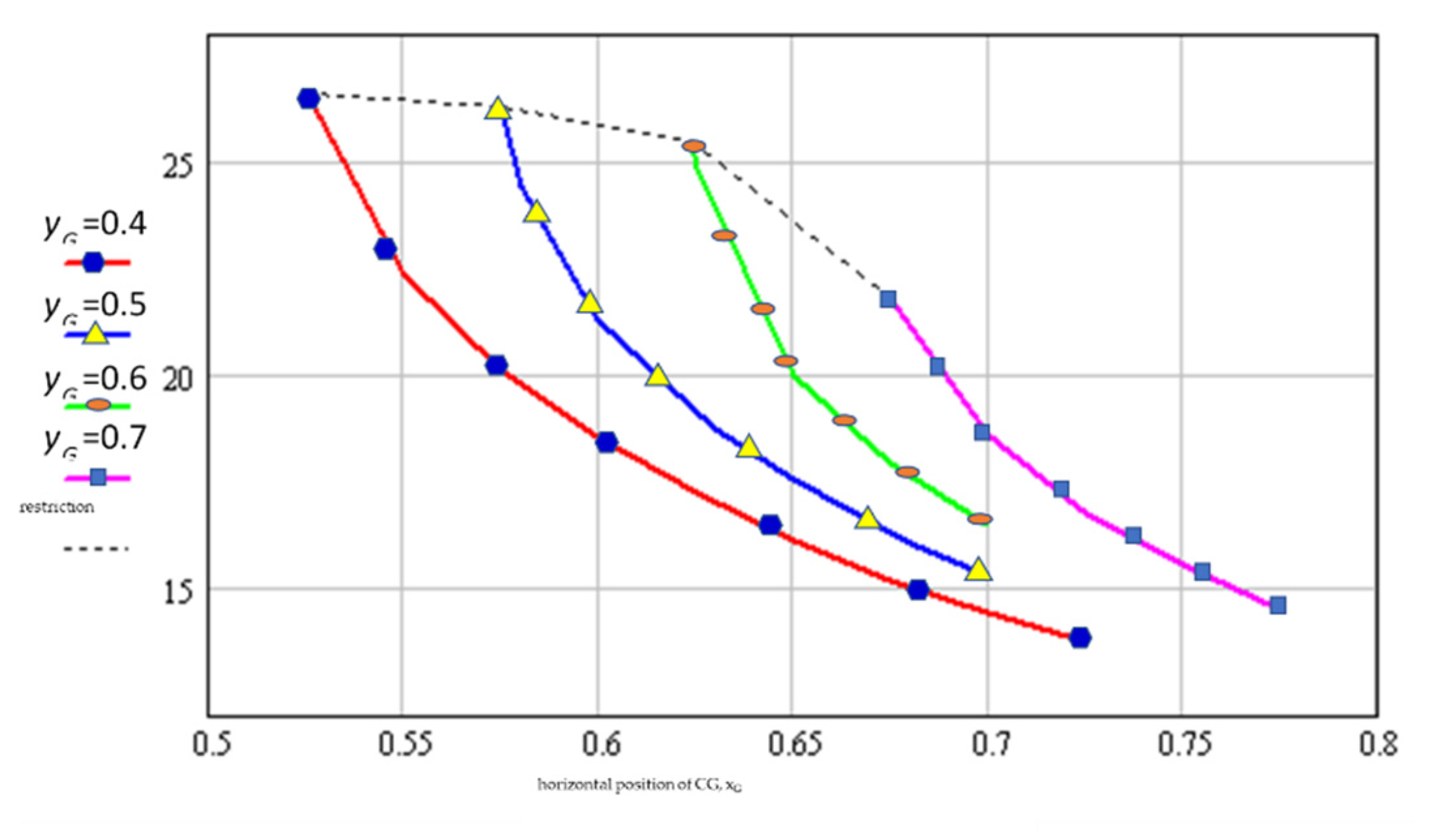
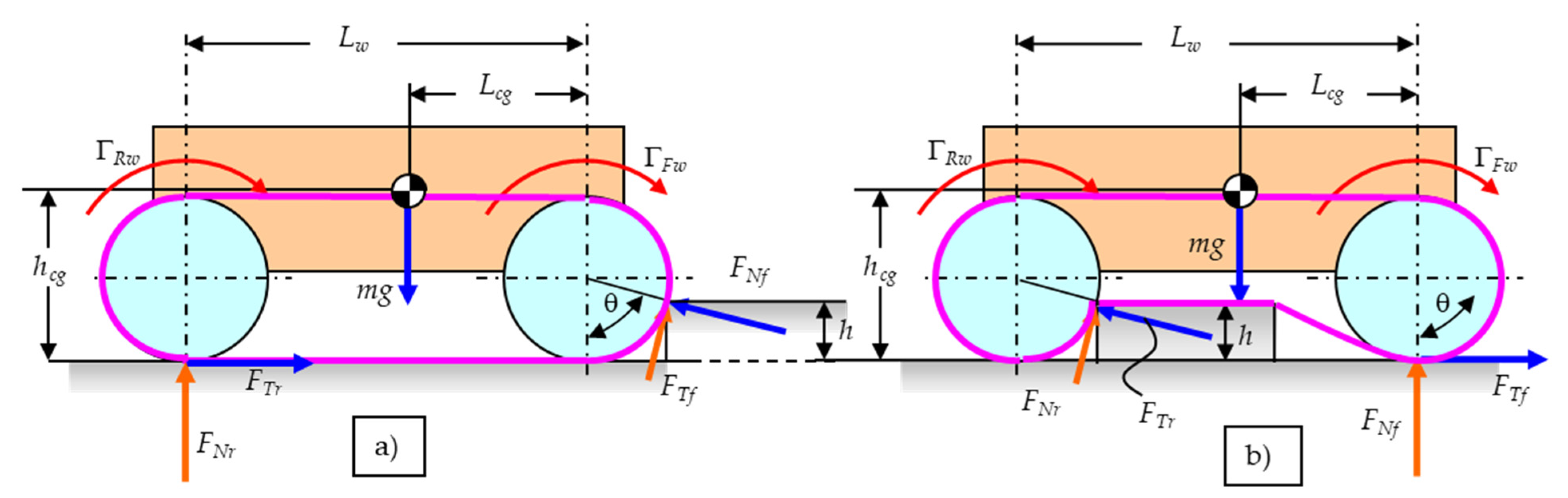
3.4. Static Stability Study of the Crawler Engine

The geometric characteristics of the crawler propeller, as well as the position of the center of mass of the mobile robot, are critical for ensuring stability in static mode: movement on the longitudinal slope; crossing the slope; turning with a stable radius; cargo handling.

From the point of view of the stability of the tracked platform when moving on the longitudinal slope, the most difficult situation occurs when braking during the descent of the slope (Figure 17), which is denoted for the deceleration of the platform during braking: $a=\frac{{\mathrm{d}}^{2}x}{\mathrm{d}{t}^2} \left[\raisebox{1ex}{$m$}\!\left/ \!\raisebox{-1ex}{$s^2$}\right.\right]$. At the limit, the misalignment x of the ground pressure center becomes equal to L-L1, so that the equation of equilibrium of the moments with respect to the point P of the forces acting on the platform results in the expression:

$$a=\frac{{\mathrm{d}}^{2}x}{\mathrm{d}{t}^2}=g\left(\frac{L-L_1}{h_g}\cos \alpha -\sin \alpha \right) \left[\raisebox{1ex}{$m$}\!\left/ \!\raisebox{-1ex}{$s^2$}\right.\right].$$

(25)

It can be concluded that the increase in the height of the center of gravity, as well as its movement towards the front of the platform leads to a substantial decrease in the braking deceleration at which the overturning occurs (Figure 18).

$$a=\frac{{\mathrm{d}}^{2}x}{\mathrm{d}{t}^2}=g\left(\frac{L-L_1}{h_g}\right) \left[\raisebox{1ex}{$m$}\!\left/ \!\raisebox{-1ex}{$s^2$}\right.\right].$$

(26)

Resuming the calculations that led to the plot of the graph presented above, we obtain the variation of the maximum deceleration when braking on the horizontal terrain, graphically presented in Figure 19.

The deceleration during braking is constant and the initial speed is v; it follows that the minimum time required for braking is given by the relation: $t_{\min }=v/a \left[s\right]$.

Stability on the transverse slope is a particular case of the issue of lateral stability. The geometric scheme, as well as the forces acting on the platform during the crossing of the slope, are shown in Figure 20. The overturning stability condition is satisfied as long as the resultant of the ground reactions is inside the support polygon:

$$y\le \frac{B+b}{2}=h_g\frac{G\sin \alpha +F_c}{G\cos \alpha } \left[m\right],$$

(27)

where F_c [N]—the centrifugal force, $b \left[m\right]$—track width; $B \left[m\right]$—track gauge; $F_C \left[N\right]$—centrifugal force.

For a transverse slope angle of 30°, it results in $h_g=0.866\cdot (B+b)$, which does not imply severe conditions.

4. Simulation Singularity Crossing Obstacles

4.1. Simulation of the Slope Ascent

In order to evaluate the simulation potential of the simulation performed on the basis of a simple 2D model, a two-axle vehicle was schematized in the situation of longitudinal displacement on the slope Figure 21.

$${\displaystyle \sum _{}^{}{F}_X=0=\mathsf{\mu }{\gamma }_r{F}_{Nf}-mg\sin \mathsf{\theta }} \left[N\right],$$

(28)

$${\displaystyle \sum _{}^{}{F}_Y=0=F_{Nr}+F_{Nf}-mg\cos \mathsf{\theta }} \left[N\right],$$

(29)

$${\displaystyle \sum _{}^{}M=0=F_{Nr}{L}_w-mg\left(L_{cg}\cos \mathsf{\theta }+h_{mg}\sin \mathsf{\theta }\right)} \left[Nm\right].$$

(30)

Equations (28)–(30) allow for the determination of the expressions for the normal forces acting on the drive wheels and of the minimum coefficient of adhesion that ensures the capitalization of the traction forces:

$$F_{Nr}=\frac{mg\left(L_{cg}\cos \mathsf{\theta }+h_{cg}\sin \mathsf{\theta }\right)}{L_w} \left[N\right],$$

(31)

$$F_{Nf}=\frac{mg\left[\left(L_w-L_{cg}\right)\cos \mathsf{\theta }-h_{cg}\sin \mathsf{\theta }\right]}{L_w} \left[N\right],$$

(32)

$$\mathsf{\mu }\ge \frac{L_w\sin \mathsf{\theta }}{\left({\gamma }_r-{\gamma }_f\right)\left(h_{cg}\sin \mathsf{\theta }+L_{cg}\cos \mathsf{\theta }\right)+{\gamma }_f{L}_w\cos \mathsf{\theta }} [-],$$

(33)

$$\mathsf{\theta }=\mathrm{arctg}\left(\frac{L_w-L_{cg}}{h_{cg}}\right) \left[\mathrm{deg}\right].$$

(34)

where: m [kg]—weight of the vehicle; F_Tr,f [N]—rear and front traction force, respectively; F_{Nr, Nf} [N]—normal force back, respectively front; θ [deg]—angle of the longitudinal slope; L_cg [m]—distance of the center of mass from the axis of the front axle; h_cg [m]—distance of the center of mass from the running surface; L_w, [m]—the distance between the axes of the axles; γ [−]—coefficient of indication of the driving axis, with value 1 if the axis is driving and 0 if the axis is not driving.

The data that were considered for the simulation are contained in

Table 2. Characteristics of the crawler robot used for simulation.

Characteristics	U.M.	Amount
Rear wheel diameter, Drw	mm	350
Front wheel diameter, Dfw	mm	350
Wheelbase, Lw	mm	1200
Distance between front axle and center of gravity, Lcg	mm	600
Height of the center of gravity relative to the running track, hmg	mm	650
The mass of the vehicle, m	kg	250
The weight of the vehicle, mg	N	2450
Coefficient of adhesion, μ	-	0.8

.

From the analysis of the obtained results, it results that the all-wheel drive solution is the most favorable.

4.2. Simulation of Crossing the Step-Type Obstacle

The simulation of crossing a step-type obstacle was performed in two variants (Figure 22): when climbing the obstacle; and suspended on the obstacle.

Using the schematic in Figure 22, the following geometric relationships are calculated:

$$\cos \theta =\frac{R-h}{R} [-], \sin \theta =\frac{\sqrt{h\left(2R-h\right)}}{R} [-]$$

(35)

The equilibrium equations for the forces and moments acting on the vehicle are as follows:

$${\displaystyle \sum {{\displaystyle F}}_X}=0=\mu {{\displaystyle \gamma }}_r{{\displaystyle F}}_{Nr}+\mu {{\displaystyle \gamma }}_f{{\displaystyle F}}_{Nf}\cos \theta -{{\displaystyle F}}_{Nf}\sin \theta \left[N\right],$$

(36)

$${\displaystyle \sum {{\displaystyle F}}_Y}=0={{\displaystyle F}}_{Nr}-mg+{{\displaystyle F}}_{Nf}\cos \theta +\mu {{\displaystyle \gamma }}_f{{\displaystyle F}}_{Nf}\sin \theta \left[N\right],$$

(37)

$${\displaystyle \sum M}=0={{\displaystyle -F}}_{Nr}\left({{\displaystyle L}}_w+R\sin \theta \right)+mg\left({{\displaystyle L}}_{cg}+R\sin \theta \right) \left[Nm\right].$$

(38)

The following notations are introduced:

$$\begin{array}{c}A=L_{CG}+R\sin \theta \left[m\right], B=L_w-L_{cg} \left[m\right], S=\sin \theta [-],\\ C=\cos \theta [-]\end{array}$$

(39)

From Equations (35)–(42), the following second-degree equation is finally obtained:

$${{\displaystyle \mathsf{\mu }}}^2{{\displaystyle \gamma }}_r{{\displaystyle \gamma }}_{f}AS+\mathsf{\mu }C\left(A{{\displaystyle \gamma }}_r+B{{\displaystyle \gamma }}_f\right)-SB=0,$$

(40)

with the next positive solution:

$$\mathsf{\mu }\ge \frac{-C\left(A{{\displaystyle \gamma }}_r+B{{\displaystyle \gamma }}_f\right)+\sqrt{{{\displaystyle C}}^2{{\displaystyle \left(A{{\displaystyle \gamma }}_r+B{{\displaystyle \gamma }}_f\right)}}^2+4{{\displaystyle \gamma }}_r{{\displaystyle \gamma }}_{f}AB{{\displaystyle S}}^2}}{2{{\displaystyle \gamma }}_r{{\displaystyle \gamma }}_{f}AS}.$$

(41)

Relationship (41) allows one to determine the coefficient of adhesion required to cross the obstacle. From Equations (36)–(38) result the expressions of the normal forces acting on the drive wheels:

$${{\displaystyle F}}_{Nr}=\frac{mgA}{{{\displaystyle L}}_w+RS} \left[N\right], F_{Nf}=\frac{mgB}{\left({{\displaystyle L}}_w+RS\right)\left(C+\mathsf{\mu }{{\displaystyle \gamma }}_{f}S\right)} \left[N\right]$$

(42)

If the obstacle is crossed by a single axis, the following equations are used:

$${\displaystyle \sum {{\displaystyle F}}_X}=0=\mu {{\displaystyle \gamma }}_r{{\displaystyle F}}_{Nr}+\mu {{\displaystyle \gamma }}_f{{\displaystyle F}}_{Nf}\cos \theta -{{\displaystyle F}}_{Nf}\sin \theta /2 \left[N\right].$$

(43)

$$\mu \ge \frac{-C\left(A{{\displaystyle \gamma }}_r+B{{\displaystyle \gamma }}_f\right)+\sqrt{{{\displaystyle C}}^2{{\displaystyle \left(A{{\displaystyle \gamma }}_r+B{{\displaystyle \gamma }}_f\right)}}^2+2{{\displaystyle \gamma }}_r{{\displaystyle \gamma }}_{f}AB{{\displaystyle S}}^2}}{2{{\displaystyle \gamma }}_r{{\displaystyle \gamma }}_{f}AS} [-].$$

(44)

$${{\displaystyle F}}_{Nr}=\frac{mgA}{{{\displaystyle L}}_w+RS} \left[N\right]., {{\displaystyle F}}_{Nf}=\frac{mgB}{\left({{\displaystyle L}}_w+RS\right)\left(C+\mu {{\displaystyle \gamma }}_{f}S\right)} \left[N\right]$$

(45)

The calculations were performed tabularly in Microsoft Excel. The results obtained are presented in

Table 3. The results of the simulation for crossing the step-type obstacle with a single track.

h, mm	50	75	100	125	150
Normal force at the rear axle wheels, N	669.2	678	684	687	689.8
Minimum adhesion coefficient, μ2, μmin2	0.2	0.26	0.33	0.41	0.51
Normal force on the front axle wheels, N	650	693	741	788	829.3
Total traction force, N	2514	2514	2514	2514	2171
Limited tensile strength of grip, N	1070	1085	1094	1100	1104

and

Table 4. The results of the simulation for crossing the step-type obstacle with a single track.

h, mm	50	75	100	125	150
Normal force at the rear axle wheels, N	669.2	678	684	688	689.8
Minimum adhesion coefficient, μ2, μmin2	0.37	0.47	0.56	0.66	0.76
Total traction force, N	2514	2514	2514	2514	2171
Limited tensile strength of grip, N	1070	1085	1094	1100	1104

.

The data obtained allow for an assessment of the demands of the driving wheels that attack the obstacle; the coefficient of adhesion required for the development of the traction force; the requirements imposed on the energy aggregate (engine and transmission) to overcome the obstacle.

From the analysis of the obtained data, it can be seen that the most important variation is the coefficient of adhesion necessary to allow for the crossing of the obstacle. For the two situations studied, Figure 23 and Figure 24 show the variation in the minimum adhesion coefficient that ensures the crossing of the obstacle, depending on its height.

As the height of the obstacle increases, so does the need for traction. The variation in the traction force required to cross the obstacle is shown in Figure 25 and Figure 26.

From the analysis of the presented graphs, it can be concluded that crossing the obstacle with both tracks leads to the increase in the required traction force with a value of about 250–350 N, approximately constant depending on the height of the obstacle.

The simulations were performed for a disposition of the center of mass, arranged symmetrically with respect to the two axes, and the traction force was evenly distributed over the entire adhesion length of the track: the model is simple and easy to operate, providing important and relevant information; the correlation between the constructive parameters and the functional characteristics is easy to highlight and to be optimized at a coarse level; the simplicity of the model makes it quickly integrated into complex models for simulating mobility.

4.3. Simulation of Crossing the Step-Type Obstacle with Recurdyn

The virtual model of a crawler engine was made using the specialized program Recurdyn. After making the virtual model, we proceeded to check the arrangement of all elements in order to eliminate interference or incorrect positioning (Figure 27).

These simulations refer to the decomposition of the traction forces on the three directions of the orthogonal axis system. Each track element (patina) displaces the tread in the three directions. The graphs in Figure 28 refer to those stated.

Simulating the contact of a skid in the composition of the track with the ground allows for the extraction of information on vertical stresses on the ground (ground pressure), as well as the evaluation of reactions in the direction of travel, which allows for the study of the ground lift in the direction of traction.

The study of the contact between the skate and the buckets allows for the evaluation of the contact force with implications for the dimensioning of the rubber bandage, but also for the identification of possible shocks when the bucket passes over two skates due to the intersection between them (Figure 29).

The simulation study of the torque variation at the driving wheel indicates its important variations, in the conditions of a stationary movement, with constant speed (Figure 30).

Studying the simulation of travel speed for a value of about 45% of the maximum travel speed indicates the existence of irregularities that can have disruptive adverse effects on the image stability recorded by the video cameras installed on the platform (Figure 31).

An attenuation of these variations will be recorded by taking into account the moment of inertia of the electric motor and gearboxes.

5. Testing and Evaluation Propulsion Systems

The following main objectives of the experimental research were determined: the functional characteristics of the mobile platform; the functional characteristics of some main components of the mobile platform;

The testing of the mobility of the mobile robot had the following important objectives: the operation of the propulsion system when moving rectilinearly; when cornering; the control mode of the controller; the operation of the engine: in reverse and reverse; at rapid changes of the operating mode; the road holding of the mobile robot.

5.1. Testing and Evaluation on the Stand

The testing of electric motors had the following objectives: the operation of motors at supply voltages of 12 Vcc and 24 Vcc; the controller and the electrical connections between the motor and the controller; the way of simultaneously changing the speed of electric motors; how to differentiate the speed of electric motors.

Stand-up testing of electric motors followed, checking the way of making the electrical connections between the motor and the controller; the RS232 and ANALOG control modes of the motors; the operation of the motors in simultaneous and differentiated speed regime; the efficiency of the engine failure stop system.

The following operations were performed prior to the actual execution of the tests (Figure 32): the smooth rotation of the shafts of the electric motors was verified; integrity of the electrical conductors connecting the electric motors was checked; motors were mounted on the test stand. The schematic of the electrical connections is included in Figure 33. The electrical connections were made with conductors of large section so as to avoid voltage drops when high currents occur.

In the case of designing the DasyLab application, a decision was made to monitor and record the measured values. Butherworth type 3 digital filters were used to reduce the noise associated with the acquired signals. A first set of data was purchased during the stand test of electric motors. Next, a vacuum test was performed at different speeds of the two engines. The results are shown in Figure 32 For these tests, the digital control of the controller was used through the RS232 interface of the computer.

From the analysis of the presented graph, the following can be noticed (Figure 34): the value of the current varies relatively little with the speed due to the fact that the mechanical load of the electric motor is zero, so that the absorbed current has relatively small values; control through the RS232 interface provided by the RoboteQ program leads to the execution of the turn by differentiating the speeds as follows: the outer track of the turn: $v+\Delta v$; and the inner track of the turn: $v-\Delta v$; where $\Delta v$ it is proportional to the turn command (Figure 35).

5.2. Engine Testing by Suspension Test

Suspended testing of electric motors followed the same things as in Section 5.1.

The results of the test for simulating rectilinear gait are shown in Figure 36.

The analysis of the graphically represented data shows the dependence between speed and absorbed current, which can be explained by the increased level of friction torque in the gearboxes.

Figure 37 shows examples of results obtained when simulating the turn in the suspended test.

The development of experimental research allowed the formulation of the following: the testing program was completed and complied with procedural requirements; when the electric motors are idle, they absorb a current of about 3 A rms; in the case of a rapid change of speed by about 10%, there were short-term increases in the absorbed current of up to 8 A rms; due to the technological and adjustment non-uniformity, the speeds of the two engines differ by about 1–2% when idling; no abnormal noises or overheating were found during the operation of the gearboxes. During the operation of the tracks, the test was suspended: the occurrence of the phenomenon of hooking the tip of the tooth flank of the crawler chain roller was noted, as the phenomenon was found both at the entry into the gear and at the exit of the gear, given that the support branch of the track is a free-forming an arrow of about 35–40 mm, as can be easily seen from Figure 38; the current absorbed by the motors, corresponding to a speed regime close to the maximum speed, by 18–20 A rms.

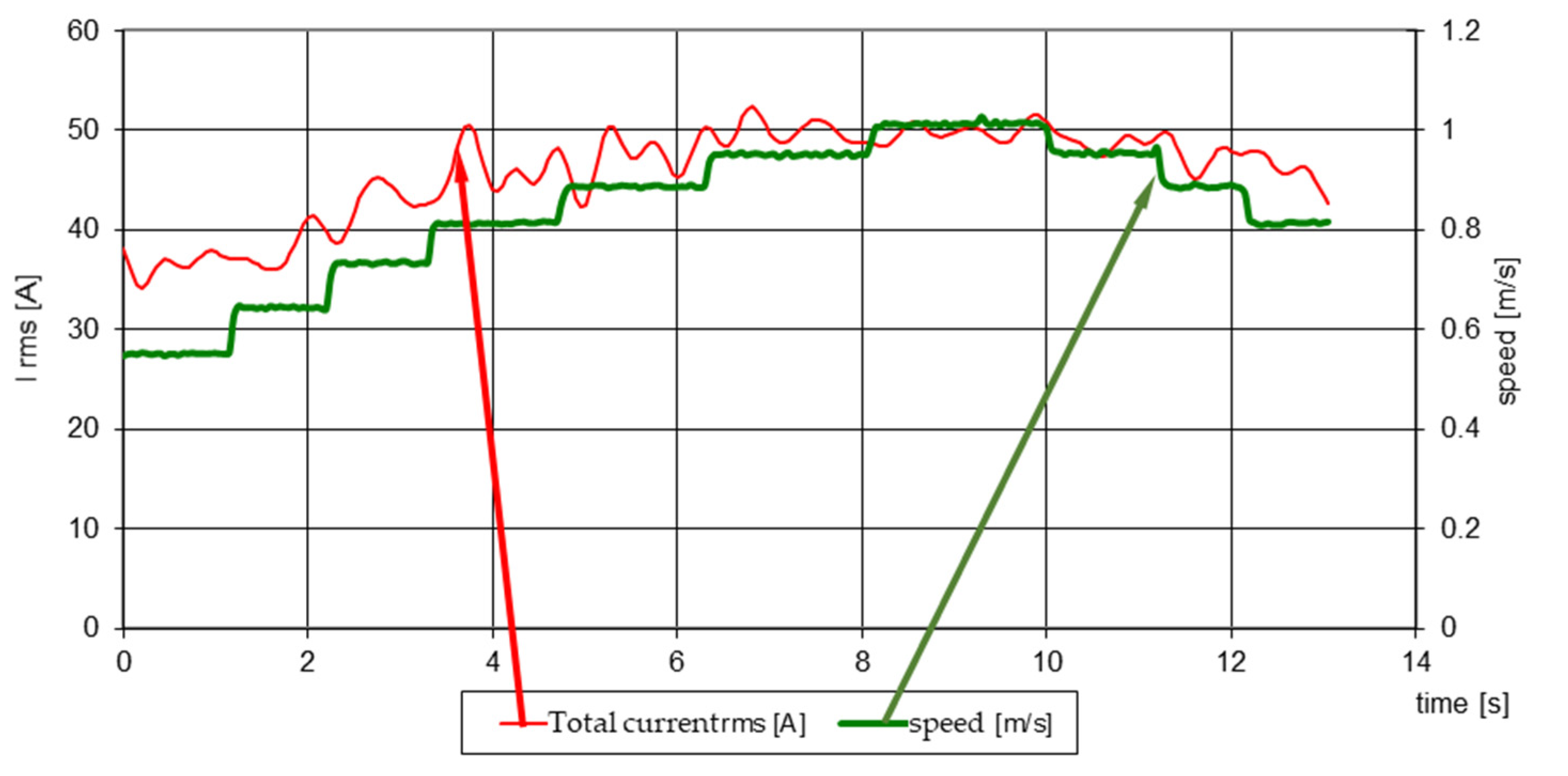
5.3. Testing and Evaluation of Rectilinear Displacement Capacity

Rectilinear gait testing was followed: testing the robot’s ability to move forward in a straight line; backwards in a straight line; the ability to accelerate the mobile robot; determination of the maximum speed. A data acquisition system assisted by a portable PC using the specialized program DasyLab was used to perform the measurements.

An example of recording data at rectilinear motion at maximum speed is shown in Figure 39. The maximum speed obtained was higher than 1 m/s.

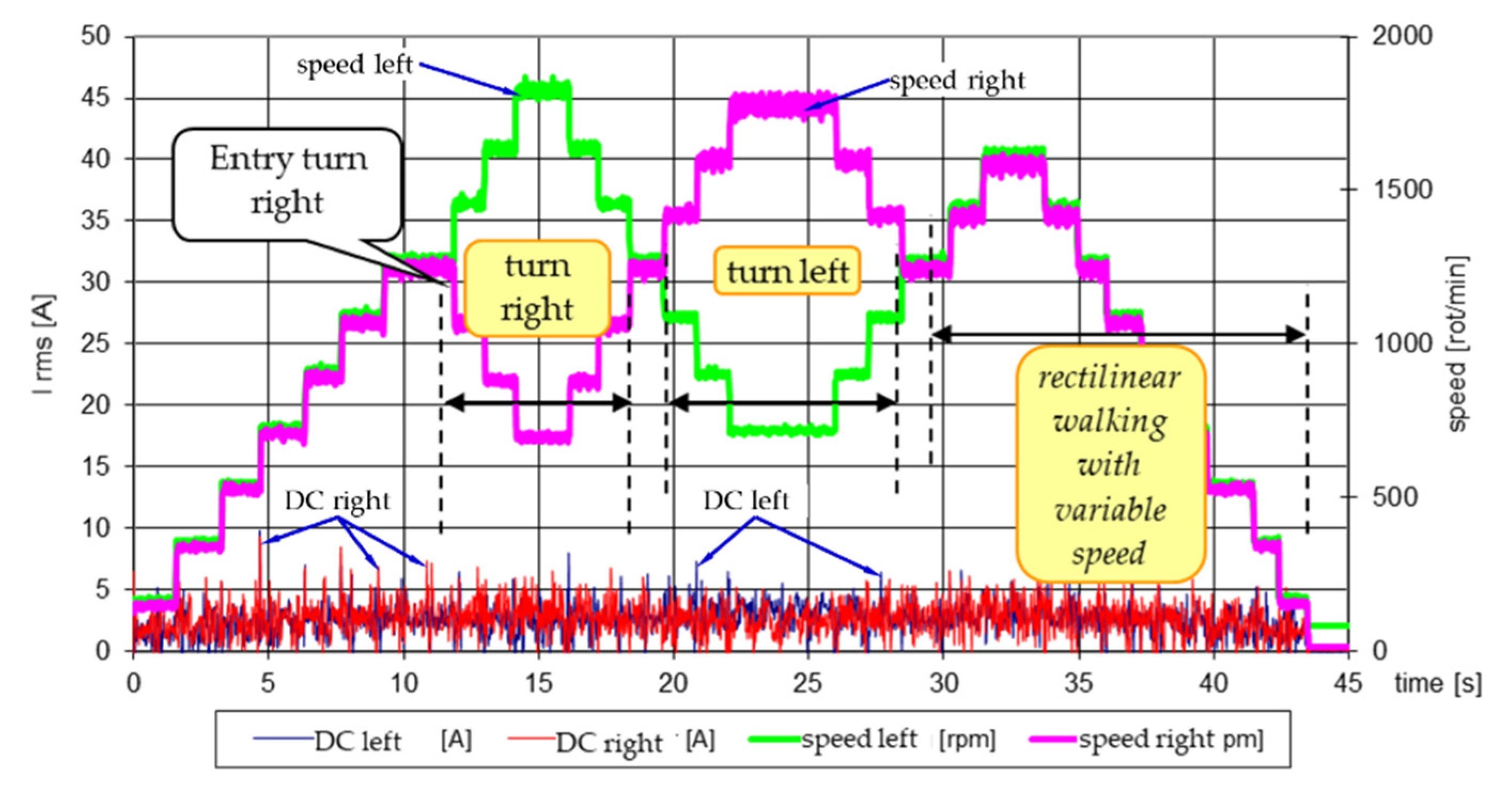
5.4. Testing and Evaluation of the Ability to Make the Turn

Testing of ability to make the turn followed the same things as in Section 5.1.

The same data acquisition systems described above were used to perform the measurements. On-the-go testing at two different engine speeds was performed by analog control, maintaining a relatively long time the command to be able to record data at constant operating speeds. During the suspended test, the following steps were performed: straight forward movement followed by turning right and then left; rectilinear movement backwards followed by the execution of the right and then left turn; execution of the turn with minimum radius only by driving only one track. In the first two stages, the following aspects were pursued: ability to make turns with different radius; the quality of the crawler gear drive; firmness and accuracy of the analog control. In the third stage, the following aspects were further pursued: ability to execute the turn with a minimum radius; smooth, noiseless operation of the tracks; control of the controller in analog mode; efficiency of the track guidance and stretching mechanism. The turning radius was determined:

$${\mathsf{\rho }}_2=B{v}_2/v_2-v_1 \left[m\right].$$

(46)

where B [m]—the gauge of the mobile robot; v [m/s]—left track speeds (index 2) and right track (index 1), respectively.

From the analysis of the graphically represented data, it is found that, at the rectilinear course for which v₂ = v₁, the turning radius tends to take an infinite value (Figure 40). During the test when performing the turn by operating a single track, it was found that a turning radius of 0.68 ÷ 0.72 (m) was achieved, depending on the landslide of the immobilized track. During testing the ability to travel for a long time, the robot performed the following travel categories for 80 min: rectilinear movement back and forth; turning left and right; crossing singular obstacles. When operating the robot at maximum speed, the electric motors absorb a current of about 50 A rms, representing less than 50% of the maximum current set for the controller (110 A) and about 35% of the maximum capacity of the controller (140 A), the values recorded differ from those determined by simulation with a maximum of 6.52%, which confirms the validity of the calculation model developed.

5.5. Experimental Research on the Ability to Approach Obstacles

Testing the ability of the mobile obstacle robot had the following more important objectives: testing the operation of the propulsion system when crossing obstacles; the control mode of the controller; the operation of the engine at rapid changes in operating mode; the road holding of the mobile robot when approaching obstacles (Figure 40).

The rectilinear gait test aimed at testing the ability to approach the obstacle in terms of energy resource and the characteristics of the track’s adhesion to the ground.

An example of data recorded at rectilinear displacement at maximum speed is shown in Figure 41. It is noted that, although the displacement speed was approximately constant (red line), the current shows significant variations due to the corresponding change in the overall resistance coefficient to advance.

The height of the obstacle was 160 mm and the average speed of approaching the obstacle was 0.363 m/s. During the obstacle approach, the absorbed current had an average value of 57.22 A with a maximum of over 120 A. During the obstacle approach the robot control was firm, and its speed remained at an approximately constant value, the variations being generated by the entry/exit of/in contact with the edges of the obstacle of the support rollers of the track.

6. Conclusions and Discussion

The engine test program was completed in full and complied with the procedural requirements. The test program had a complex character, including the running of motors, reducers and tracks. When the electric motors are idle, they absorb a current of about 3 rms. In the case of a rapid change in speed of about 10%, there were short-term increases in the absorbed current of up to 8 A rms.

When operating during the test, the current absorbed by the motors, corresponding to a speed regime close to the maximum speed, was suspended at 18–20 A rms. Thus, regardless of the speed regimes, when driving in a straight line and/or in a corner, as well as for both directions, no warm-ups of the motors or reducers were found. The temperature of the MOSFET power components in the controller exceeded the ambient temperature by 1–2 °C. The values of the absorbed current represent 12–15% of the maximum current allowed by the controller.

The values obtained differ from those calculated by a simulation with a maximum of 4.7%. Increased current values were recorded at the transient regimes. The tests followed the following functional algorithm:

Through the program of experimental research, the following important issues related to the functional characteristics of the mobile platform were revealed: the constructive characteristics of the ROBTER crawler robot allowed for stable and fully controllable rolling; the ROBTER crawler robot did not lose its grip, and there was no skidding or tilting; the ability to cross the individual obstacles (longitudinal slope) of the ROBTER crawler robot is considered to be in accordance with the formulated requirements;

The main advantages of the studied solution are the possibility of creating a family of intervention robots by replacing the operational platform; simplicity of the calculation logarithm; making modular software; the use of relatively cheap materials and components, the aim being to increase the degree of efficiency and annihilation of potential risks with minimal costs. In addition, this functional model can also be used for research activities in the subject, as well as for doctorates. As the structure is extremely versatile, future users develop it to conduct in-depth research. In further research, we want to focus on describing the influence of the crawler propeller on the ground and on the development of at least two new operational platforms.

The previously-performed and presented study had as main objective the highlighting of the influences that the main geometric parameters exert on the functional characteristics of the mobile robot. The following conclusions regarding the geometric configuration of the mobile robot platform result: the increase in the height at which the center of mass is arranged leads to more favorable conditions for approaching step-type obstacles but generates conditions of loss of stability when sloping and braking, especially when braking when descending the slope; increasing the height of the axis of the drive wheel leads to the corresponding increase of the height of the step-type obstacle that can be approached, but also to the increase of the width of the ditch that can be crossed; the forward movement of the horizontal position of the center of gravity leads to more advantageous conditions for tackling step-type obstacles, but appropriately reduces the width of the ditch that can be crossed and increases the value of the forces required to perform the turn; increasing the adhesion length of the crawler propeller with the ground leads to the corresponding increase in the width of the ditch that can be crossed but also to the increase in the traction forces in turning; the increase of the track width allows to obtain a lower average pressure on the ground, reducing the sinking of the tracked propeller in the deformable ground and, therefore, the resistance to advance; the lower sinking in the deformable soil also leads to the reduction of the lateral excavation effect during the execution of the turn, which leads to the decrease of the resistance moment in the turn.

All these conclusions highlight the contradictory nature of the influence exerted by the main geometric parameters of the crawler engine on the functional characteristics of the mobile robot. This results in the need to optimize the geometrical parameters of the crawler engine according to the characteristics of the specific mission for which the mobile robot is intended. All these considerations were taken into account when making the prototype, which is the subject of this paper.

References

1. Luxton, A.; Marinov, M. Terrorist Threat Mitigation Strategies for the Railways. Sustainability 2020, 12, 3408. [Google Scholar] [CrossRef] [Green Version]
2. Kaewunruen, S.; Alawad, H.; Cotruta, S. A Decision Framework for Managing the Risk of Terrorist Threats at Rail Stations Interconnected with Airports. Safety 2018, 4, 36. [Google Scholar] [CrossRef] [Green Version]
3. Kanji, A. Framing Muslims in the “War on Terror”: Representations of Ideological Violence by Muslim versus Non-Muslim Perpetrators in Canadian National News Media. Religions 2018, 9, 274. [Google Scholar] [CrossRef] [Green Version]
4. Gibbs, J.P. Conceptualization of Terrorism. Am. Sociol. Rev. 1989, 54, 329–340. [Google Scholar] [CrossRef]
5. Eikenberry, K.W. Thoughts on Unconventional Threats and Terrorism; Working Group on Foreign Policy and Grand Strategy, Hoover Institution, Stanford University: Stanford, CA, USA, 2014. [Google Scholar]
6. Available online: https://ec.europa.eu/echo/files/about/COMM_PDF_SEC_2010_1626_F_staff_working_document_en.pdf (accessed on 18 February 2021).
7. National Research Council. Technology Development for Army Unmanned Ground Vehicles. ISBN: 0-309-08620-5. Available online: http://www.nap.edu/catalog/10592.html (accessed on 22 February 2021).
8. Available online: https://www.unodc.org/e4j/en/terrorism/module-4/key-issues/defining-terrorism.html (accessed on 17 March 2021).
9. Cassese, A. The Multifaceted Criminal Notion of Terrorism in International Law. JICJ 2006, 4, 933–958. [Google Scholar] [CrossRef]
10. Dewulf, S. Human Rights in the Criminal Code: A Critique of the Curious Implementation of the EU and Council of Europe Instruments on Combating and Preventing Terrorism in Belgian Criminal Legislation. EJC CLCJ 2014, 22, 33–57. [Google Scholar] [CrossRef]
11. Liem, M.; van Buuren, J.; de Roy van Zuijdewijn, J.; Schönberger, H.; Bakker, E. European Lone Actor Terrorists Versus “Common”. Homicide Stud. 2018, 22, 45–69. [Google Scholar] [CrossRef] [Green Version]
12. Available online: https://www2.ohchr.org/english/bodies/chr/special/counter-terrorism.htm (accessed on 15 March 2021).
13. Duquet, N.; Goris, K. Firearms Acquisition by Terrorists in Europe, Research Findings and Policy Recommendations of Project SAFTE; Flemish Peace Institute: Brussels, Belgium, 2018; ISBN 9789078864912. [Google Scholar]
14. Available online: https://govinfo.library.unt.edu/911/report/911Report_Exec.htm (accessed on 2 March 2021).
15. Czop, A.; Hacker, K.; Murphy, J.; Zimmerman, T. Low-cost explosive ordnance disposal robot using off-the-shelf parts. In Proceedings of the Unmanned Ground Vehicle Technology VII, Defence and Security, Orlando, FL, USA, 27 May 2005; Volume 5804. [Google Scholar] [CrossRef]
16. Available online: https://www.un.org/sc/ctc/wp-content/uploads/2017/03/CTED-Trends-Report-March-2017-Final.pdf (accessed on 10 March 2021).
17. Van Moore, A., Jr. Radiological and nuclear terrorism: Are you prepared? Am. Coll. Radiol. 2004, 1, 54–58. [Google Scholar] [CrossRef]
18. Available online: https://www.ouvry.com/en/nrbce-terrorist-chemical-weapons-attacks/ (accessed on 2 March 2021).
19. Maynard, R.M.; Tetley, T.D. Bioterrorism: The lung under attack. 2004, 59, 188–189. [Google Scholar] [CrossRef] [Green Version]
20. Available online: https://www.un.org/sc/ctc/wp-content/uploads/2019/01/Compendium_of_Good_Practices_Compressed.pdf (accessed on 2 March 2021).
21. Paulius, D.; Sun, Y. A Survey of Knowledge Representation in Service Robotics. Robot. Auton. Syst. 2019, 118, 13–30. [Google Scholar] [CrossRef] [Green Version]
22. Matuszek, C.; Herbst, E.; Zettlemoyer, L. Learning to parse natural language commands to a robot control system. In Experimental Robotics; Desai, J., Dudek, G., Khatib, O., Kumar, V., Eds.; Springer: Berlin/Heidelberg, Germany, 2016; Volume 88, pp. 403–415. [Google Scholar]
23. Liu, R.; Webb, J.; Zhang, X. Natural-Language-Instructed Industrial Task Execution. In Proceedings of the ASME IDETC/CIE, Charlotte, NC, USA, 21–24 August 2016; p. v01bt02a043. [Google Scholar]
24. Tay, N.N.W.; Saputra, A.A.; Botzheim, J.; Kubota, N. Service robot planning via solving constraint satisfaction problem. Robomech. J. 2016, 3, 17. [Google Scholar] [CrossRef] [Green Version]
25. Zhang, S.; Sridharan, M.; Wyatt, J.L. Mixed logical inference and probabilistic planning for robots in unreliable worlds. IEEE Trans. Robot. 2015, 31, 699–713. [Google Scholar] [CrossRef] [Green Version]
26. Kress-Gazit, H.; Wongpiromsarn, T.; Topcu, U. Correct, reactive robot control from abstraction and temporal logic specifications. IEEE Robot. Autom. Mag. Spec. Issue Form. Methods Robot. Autom. 2011, 18, 65–74. [Google Scholar] [CrossRef]
27. Xie, M. Robot Vision: A Holistic View. In Climbing and Walking Robots; Springer: Berlin/Heidelberg, Germany, 2005. [Google Scholar] [CrossRef]
28. Carey, M.W.; Kurz, E.M.; Matte, J.D.; Perrault, T.D. Novel EOD Robot Design with a Dexterous Gripper and Intituitive Teleoperation. In Proceedings of the World Automation Congress 2012, Puerto Vallarta, Mexico, 24–28 June 2012; IEEE: New York, NY, USA, 2012; Volume 1, pp. 463–469. ISBN 9781467344975. [Google Scholar]
29. Belanche, D.; Casaló, L.V.; Flavián, C.; Schepers, J. Service robot implementation: A theoretical framework and research agenda. Serv. Ind. J. 2020, 40, 203–225. [Google Scholar] [CrossRef] [Green Version]
30. Saputra, R.P.; Rijanto, E. Automatic Giuded Vehicles System and Its Coordination Control for Containers Terminal Logistics Application. Conf. Int. Logist. Semin. Workshop 2012, 2, 4. [Google Scholar]
31. Grigore, L.Ș.; Priescu, I.; Grecu, D.L. Inteligența Artificială Aplicată în Sisteme Robotizate Fixe și Mobile; Editura AGIR: Bucuresti, Romania, 2020; p. 703. ISBN 978-973-720-767-8. [Google Scholar]
32. Grigore, L.Ș.; Gorgoteanu, D.; Molder, C.; Alexa, O.; Oncioiu, I.; Ștefan, A.; Constantin, D.; Lupoae, M.; Bălașa, R.I. A Dynamic Motion Analysis of a Six-Wheel Ground Vehicle for Emergency Intervention Actions. Sensors 2021, 21, 1618. [Google Scholar] [CrossRef]
33. Deng, W.; Zhang, H.; Li, Y.; Gao, F. Research on target recognition and path planning for EOD robot. Int. J. Comput. Appl. Technol. 2018, 57, 325–333. [Google Scholar] [CrossRef]
34. Rajan, K.; Saffiotti, A. Towards a science of integrated AI and robotics. Artif. Intell. 2017, 247, 1–9. [Google Scholar] [CrossRef] [Green Version]
35. Dudzik, S. Application of the Motion Capture System to Estimate the Accuracy of a Wheeled Mobile Robot Localization. Energies 2020, 13, 6437. [Google Scholar] [CrossRef]
36. Russo, M.; Raimondi, L.; Dong, X.; Axinte, D.; Kell, J. Task-oriented optimal dimensional synthesis of robotic manipulators with limited mobility. Robot. Comput. Integr. Manuf. 2021, 69, 102096. [Google Scholar] [CrossRef]
37. Sandry, E. Robots and Communication, 1st ed.; Palgrave Macmillan: London, UK, 2015; p. 129. ISBN 978-1-137-46837-6. [Google Scholar] [CrossRef]
38. Zhao, J.; Gao, J.; Zhao, F.; Xu, Z.; Liu, Y. A design Method for Multijoint Explosive-Proof Manipulators by Two Motors. Appl. Sci. 2018, 8, 712. [Google Scholar] [CrossRef] [Green Version]
39. Jian-Jun, Z.; Ru-Qing, Y.; Wei-Jun, Z.; Xin-Hua, W.; Jun, Q. Research on Semi-Automatic Bomb Fetching for an EOD Robot. Int. J. Adv. Robot. Syst. 2007, 4, 27. [Google Scholar] [CrossRef]
40. Chatziparaschis, D.; Lagoudakis, M.G.; Partsinevelos, P. Aerial and Ground Robot Collaboration for Autonomous Mapping in Search and Rescue Missions. Drones 2020, 4, 79. [Google Scholar] [CrossRef]
41. Liao, J.-C.; Chen, S.-H.; Zhuang, Z.-Y.; Wu, B.-W.; Chen, Y.-J. Designing and Manufacturing of Automatic Robotic Lawn Mower. Processes 2021, 9, 358. [Google Scholar] [CrossRef]
42. Chen, X.; Huang, F.; Zhang, Y.; Chen, Z.; Liu, S.; Nie, Y.; Tang, J.; Zhu, S. A Novel Virtual-Structure Formation Control Design for Mobile Robots with Obstacle Avoidance. Appl. Sci. 2020, 10, 5807. [Google Scholar] [CrossRef]
43. Alexa, O.; Coropețchi, I.; Vasile, A.; Oncioiu, I.; Grigore, L.Ș. Considerations for determining the coefficient of inertia masses for a tracked vehicle. Sensors 2020, 20, 5587. [Google Scholar] [CrossRef]
44. Niu, J.; Wang, H.; Shi, H.; Pop, N.; Li, D.; Li, S.; Wu, S. Study on structural modeling and kinematics analysis of a novel wheel-legged rescu robot. IJARS 2018, I-17, 17. [Google Scholar] [CrossRef] [Green Version]
45. Islam, A.J.; Alam, S.S.; Ahammad, K.T.; Nadim, F.K.; Barua, B. Design, kinematic and performance evaluation of a dual arm bomb disposal robot. In Proceedings of the 2017 3rd EICT, Khulna, Bangladesh, 7–9 December 2017; pp. 1–6. [Google Scholar] [CrossRef]
46. Scalera, L.; Palomba, I.; Wehrle, E.; Gasparetto, A.; Vidoni, R. Natural Motion for Energy Saving in Robotic and Mechatronic Systems. Appl. Sci. 2019, 9, 3516. [Google Scholar] [CrossRef] [Green Version]
47. Lei, C.; Chang, F.; Li, S.; Zhang, X. Control System of the Explosive Ordnance Disposal Robot Based on Active Eye-to-Hand Binocular Vision, Artificial Intelligence and Computational Intelligence; Springer: Berlin/Heidelberg, Germany, 2011; Volume 7004, ISBN 978-3-642-23895-6. [Google Scholar]
48. Available online: https://www.nationaldefensemagazine.org/articles/2019/2/15/harris-provides-eod-robots-to-british-army (accessed on 2 March 2021).
49. Yin, Q.; Xiong, Z.; Song, S.; Zhang, G. Modular design method of EOD robot based on genetic algorithm. Int. J. Wirel. Mob. Comput. 2018, 15. [Google Scholar] [CrossRef]
50. Available online: https://ceias.nau.edu/capstone/projects/EE/2018/OrdnanceDisposal2/design_subsystems.html (accessed on 2 March 2021).
51. Available online: https://www.militarysystems-tech.com/taxonomy/term/78 (accessed on 2 March 2021).
52. Yu, J.; Jiang, W.; Luo, Z.; Yang, L. Application of a Vision-Based Single Target on Robot Positioning System. Sensors 2021, 21, 1829. [Google Scholar] [CrossRef]
53. Ștefan, A.; Constantin, D.; Grigore, L.Ș. Aspects of kinematics and dynamics of a gripping mechanism. In Proceedings of the 2015 7th ECAI, Bucharest, Romania, 25–27 June 2015; IEEE: New York, NY, USA, 2015; pp. WF1–WF4. [Google Scholar] [CrossRef]
54. Available online: https://www.ocean-comms.com.sg/product/portable-xray/ (accessed on 10 March 2021).
55. Ceccarelli, M.; Gasparetto, A. Mechanism Design for Robotics. Robotics 2019, 8, 30. [Google Scholar] [CrossRef] [Green Version]
56. Toma, Ș.A.; Sebacher, B.; Focșa, A. On Anomalous Deformation Profile Detection through Supervised and Unsupervised Machine Learning. In Proceedings of the 2019 IEEE International Geoscience and Remote Sensing Symposium, Yokohama, Japan, 28 July–2 August 2019. [Google Scholar] [CrossRef]
57. Xu, L.; Zhang, L.; Zhao, J.; Kim, K. Cornering Algorithm for a Crawler In-Pipe Inspection Robot. Symmetry 2020, 12, 2016. [Google Scholar] [CrossRef]
58. Available online: https://www.antiterrorism.eu/portfolio-posts/expert/ (accessed on 20 March 2021).
59. Grigore, L.Ș.; Ileri, R.; Neculăescu, C.; Soloi, A.; Ciobotaru, T.; Vînturiș, A. A class of autonomous robots prepared for unfriendly sunny environment. In Proceedings of the CAR2011—2011 3rd International Asia Conference on Informatics in Control, Automation and Robotics, Xiamen, China, 25–26 June 2011; Volume 646. [Google Scholar]
60. Bruch, M.H.; Laird, R.T.; Everett, H.R. Challenges for Deploying Man-Portable Robots into Hostile Environments; Space and Naval Warfare Systems Center: San Diego, CA, USA, 2001. [Google Scholar] [CrossRef] [Green Version]
61. Ogorkiewicy, R.M. Technology of Tanks; Jane’s Information Group: Coulsdon, UK, 1991; Volume 1–2, p. 424. ISBN 978-0710605955. [Google Scholar]
62. Haueisen, B. Mobility Analysis of Small, Lightweight Robotic Vehicles; Brooke Haueisen: Huntington Beach, CA, USA, 2003; p. 46. [Google Scholar]
63. Johnson, C.P. Comparative Analysis of Lightweight Robotic Wheeled and Tracked Vehicle. Ph.D. Dissertation, Virginia Polytechnic Institute and State University, Blacksburg, VA, USA, 26 April 2012; p. 155. [Google Scholar]
64. Gigler, J.K.; Ward, S.M. A simulation model for the prediction of the ground pressure distribution under tracked vehicles. J. Terramechanics 1993, 30, 461–469. [Google Scholar] [CrossRef]
Figure 1. Examples of robotic structures, including for EOD missions: (1). https://www.nides.cz/en/telerob/ (accessed on 18 February 2021); (2). https://icortechnology.com/robots/caliber-t5/caliber-t5-swat-eod-robot-leveled/ (accessed on 18 February 2021); (3). https://www.rvconnex.com/eod-robot/ (accessed on 18 February 2021); (4). https://www.publictechnology.net/articles/news/introducing-harris-t7-%E2%80%93-mod%E2%80%99s-new-%C2%A31m-bomb-disposal-robot (accessed on 18 February 2021).
Applsci 11 03757 g001
Figure 2. The general structure of an EOD mobile robot [https://www.telerob.com/en/products/teodor-evo (accessed on 18 February 2021)] mechanical and drive system [38]; location system [39]; environmental perception and security system [40]; data interpretation and task management system [41]. Operation in the environment is defined by agility and maneuverability: agility is the ability of the mobile robot to overcome obstacles [42]; maneuverability is defined by the minimum area required for a maneuver [43].
Applsci 11 03757 g002
Figure 3. Representation of different types of environmental effects on the crawler engine [59]. This representation aims to allow us to establish algorithms for defining the kinematic and dynamic model depending on the type of terrain on which the crawler robot will move.
Applsci 11 03757 g003
Figure 4. Geometric diagramming of the robot while approaching the step-type obstacle.
Applsci 11 03757 g004
Figure 5. Representation of the beginning of the climbing of high obstacles by the robot.
Applsci 11 03757 g005
Figure 6. Variation in the minimum coefficient of friction required for escalating the step obstacle. Four different values were considered for the report γ = r m / L [ ] to highlight how the CG position leads to a change in the coefficient of friction between the tracked thruster and the obstacle μ.
Applsci 11 03757 g006
Figure 7. Schematic of the ascent of the step-type obstacle, considering that the lower branch of the track is already ascended on the obstacle. Explaining notations: d [ m ] —distance from the wheel axle to the point where the lower track branch is tangent to the obstacle edge; s [ m ] —distance from the wheel axle to the point where the lower track branch is tangent to the obstacle edge; θ [ deg ] —the angle of inclination of the longitudinal axis (of the track) with respect to the running surface in the conditions in which the lower branch of the track has already “climbed” on the obstacle; s G [ m ] —the horizontal distance between the rear point of contact and the edge of the obstacle.
Applsci 11 03757 g007
Figure 8. Graphical representation of Equations (9)–(12). The variations inf the two graphs mean that, as the obstacle escalates, the distance increases s G horizontally between the rear point of contact and the edge of the obstacle decreases to zero, at which point it can be stated that the robot remains stable at the obstacle stage and the distance s from the center of the driving wheel to the point where the lower branch of the track is tangent to the edge of the obstacle is moving towards the point of minimum, and “0”, followed with increasing distance from the edge of the obstacle, the proximity of the edge following the corresponding allure.
Applsci 11 03757 g008
Figure 9. Angle variation with the horizontal position of the center of mass for h = 0.20 m, depending on y G . The variation in the inclination angle of the longitudinal axis (of the caterpillar) is obviously θ compared to the running surface in the conditions in which the lower branch of the track has already “climbed” on the obstacle, in the sense that the increase in the CG height, compared to the axle Oy, leads to increased angle θ , enabling (exaggerating) the robot to overturn.
Applsci 11 03757 g009
Figure 10. Angle variation with the horizontal position of the center of mass for h = 0.15 m. Additionally, in this case, in which the height of the step obstacle has changed (reducing it), the allure of variation of θ according to y G [ m ] is similar; only the dimensions differ.
Applsci 11 03757 g010
Figure 11. Geometric schematization of the limit situation when crossing the ditch. The explanations of the notation in the figure are: L S [ m ] —the width of the ditch; φ [ deg ] —the angle of rotation of the CG relative to the vertical line passing through the CG and the point of contact with the first edge of the ditch; h r [ m ] —the radius of a bucket.
Applsci 11 03757 g011
Figure 12. Variation of the maximum width of the ditch that can be crossed depending on the horizontal position of the center of mass.
Applsci 11 03757 g012
Figure 13. Graph of the variation of the average pressure on the ground depending on the width of the track and the length of adhesion. The simple explanation of the graph is as follows: as the width of the track b (m) and the length of the adhesion (track) increase La (m), the average pressure on the ground decreases.
Applsci 11 03757 g013
Figure 14. Behavior of a crawler vehicle with elastic suspension versus one with rigid suspension [64]; Figure 8. We cannot draw an exhaustive conclusion on which suspension system.
Applsci 11 03757 g014
Figure 15. Variation of the coefficient k as a function of the relative displacement of the center of mass xr = x/La, for La = 1.0 m. The significance of the graph lies in the fact that, with the change in the CG, in the longitudinal plane, the turning radius increases.
Applsci 11 03757 g015
Figure 16. Variation of the specific force at the inner track of the turn. The representations of the five graphs show that, as the ratio increases L a B   [ ] , the traction forces required to make the turn decrease. The observation itself is useful for determining energy consumption, f = 0.1 [−]; G = 1962 [N]; μmax = 0.5 [−].
Applsci 11 03757 g016
Figure 17. Schematic of the forces acting on the braking during the descent of the longitudinal slope. R f — the force of resistance corresponding to the contact area of the track with the ground in front of the drive wheel; R — the force of resistance corresponding to the contact area of the track with the ground in front of the bucket; N —the normal force; α —the angle of the slope.
Applsci 11 03757 g017
Figure 18. The variation of the maximum deceleration when braking on the slope of 30° depending on the position of the center of mass. It is observed that with enlargement y G and the movement of CG towards the front of the robot in the longitudinal plane, when descending the slope, we will obtain a lower deceleration until the moment that coincides with the overturning of the robot.
Applsci 11 03757 g018
Figure 19. Variation in the maximum deceleration when braking in horizontal terrain (30° slope) depending on the position of the center of mass. These simulations were performed to predict how the robot would react if it was equipped with an arm used to transport suspicious objects.
Applsci 11 03757 g019
Figure 20. Schematic of the forces acting on the robot’s platform when crossing the slope.
Applsci 11 03757 g020
Figure 21. Schematic diagram of the vehicle moving on the longitudinal slope.
Applsci 11 03757 g021
Figure 22. Schematic of crossing a step-type obstacle: (a) shows the passage over the obstacle with the first cheek, in front of the robot; (b) follows the approach of the obstacle with the driving wheel.
Applsci 11 03757 g022
Figure 23. Variation in the minimum coefficient of adhesion when crossing the obstacle with a single track. The obstacle was positioned so that only one track could be passed over it.
Applsci 11 03757 g023
Figure 24. Minimum variation coefficient of adhesion crossing an obstacle with both tracks.
Applsci 11 03757 g024
Figure 25. Variation in traction force when crossing the obstacle with a single track.
Applsci 11 03757 g025
Figure 26. Variation in traction force when crossing the obstacle with both tracks.
Applsci 11 03757 g026
Figure 27. Detail representing the crawler gearing with the drive wheel. The simulation was performed using Recurdyn software.
Applsci 11 03757 g027
Figure 28. Simulation study of track contact with the ground.
Applsci 11 03757 g028
Figure 29. Study of the contact of a patina in the composition of the caterpillar with the buckets.
Applsci 11 03757 g029
Figure 30. Simulation study of the moment at the drive wheel.
Applsci 11 03757 g030
Figure 31. Study by simulation of travel speed.
Applsci 11 03757 g031
Figure 32. How to mount the motors and the controller on the stand.
Applsci 11 03757 g032
Figure 33. Diagram of electrical connections for connecting motors.
Applsci 11 03757 g033
Figure 34. Vacuum testing at constant speed of electric motors.
Applsci 11 03757 g034
Figure 35. Vacuum testing at variable speed of electric motors.
Applsci 11 03757 g035
Figure 36. Example of recording for the simulation of rectilinear motion in the suspended sample.
Applsci 11 03757 g036
Figure 37. Example of simulating the turn in the suspended test.
Applsci 11 03757 g037
Figure 38. Overview of the mobile platform of the robot with the lower branch of the track hanging, with an arrow within the admissible limits on making the turn.
Applsci 11 03757 g038
Figure 39. Example of data recorded at rectilinear displacement.
Applsci 11 03757 g039
Figure 40. Appearance during the test of the ability to move over a rectangular prism.
Applsci 11 03757 g040
Figure 41. Example of data recorded at rectilinear displacement.
Applsci 11 03757 g041