Covert Anti-Jamming Communication Based on Gaussian Coded Modulation

Abstract

In several wireless communication systems, robustness against jammers and covertness against eavesdroppers are required simultaneously. In this paper, we propose a novel covert anti-jamming communication system. The properties of both anti-jamming and covertness are achieved through the Gaussian-coded time-frequency modulation scheme. We propose two receiver algorithms based on the sparse signal recovery framework. The receiver algorithms estimate and remove the jamming signal from the received signal. In addition, it is difficult to distinguish the proposed signal from the actual Gaussian noise in both the time and frequency domains. We compare the covertness of the proposed communication system with that of a conventional digital modulation system in terms of the probability of detection. We numerically evaluated the bit error rate of the proposed system to demonstrate its anti-jamming performance.

1. Introduction

Wireless communication systems (WCSs) have become an essential part of the infrastructure for exchanging information. However, WCSs are exposed to various threats due to the open nature of wireless media. One of these threats is eavesdropping. Eavesdroppers means malicious receivers that harm innocent users using information on the radio transmission. Since the advent of wireless communication, security to prevent damage caused by eavesdroppers has been considered an important concern.

Computational complexity-based approaches at the application layer (e.g., encryption) have been implemented for security. However, such methods are not suitable for wireless networks that contain devices with low computational power. Physical layer security, which exploits the physical properties of the wireless channel, is another solution. The random nature of the channel makes physical layer security possible. Since Wyner defined the wire-tap channel model and secrecy criterion [1], a number of researchers have studied this approach to secrecy.

The aforementioned secrecy criterion is often referred to as (physical layer) information-theoretic security. Information-theoretic security defines how much information in a confidential message is revealed to eavesdroppers. However, sometimes the presence of a communication itself should be hidden from eavesdroppers. One example is a covert military communication in a hostile region. Eavesdroppers can recognize the covert operation by detecting the presence of the signal. To evade such threats posed by eavesdroppers, a low probability of detection (LPD) for covert communications has been considered as another secrecy criterion.

Covert communication [2,3] has received little attention, relative to its importance. Without covert communications, the physical location of wireless transmitters can be detected by an eavesdropper, owing to the wireless transmission of signals. In such scenarios, the presence of wireless communications should not be easily detectable by hostile eavesdroppers.

Intentional electromagnetic radiation, also called jamming, is another serious threat to the robustness of WCSs. Jamming attacks can disturb ongoing wireless communications by causing additional errors. Jamming attacks can become more destructive if the jammers cooperate with eavesdroppers. A follower jammer [4] is an example of such cooperation. It first measures the time-frequency band of the target signal and then concentrates its jamming energy onto that band. Covert communication decreases damage by jammers using the eavesdropping-and-jamming strategy by preventing the leakage of system parameters. Thus, to protect the security and robustness of WCSs, covertness and anti-jamming performances are required simultaneously.

A spread spectrum (SS) scheme is one common solution for overcoming jamming attacks in the physical layer. Through this scheme, the bandwidth of band-limited jamming becomes much smaller than that of the communication signals. Furthermore, the scheme makes communication difficult to detect by hiding communication signals under the noise level, thus reducing the threat of eavesdroppers and eavesdropper-aided smart jammers such as follower jammers.

The coded modulation method using Gaussian-distributed code can be a complement to the SS scheme. If the modulated symbols follow a Gaussian distribution, it is difficult for the eavesdropper to distinguish whether there is a communication signal or not without an exact codebook. Furthermore, the legitimate receiver can use the error-correction property of the coding scheme. The idea of real-valued channel coding has been used, and is known as analog coding [5]. The code can correct sparse errors (e.g., narrowband jamming). Researchers [6] have studied a generalization of this coding scheme: a complex-field coding using orthogonal frequency-division multiplexing (OFDM). Candes and Tao [7] proposed a sparse error-correction method for an arbitrary generator matrix, which is a polynomial–time linear programming method unified within a compressive sensing (CS) recovery framework [8]. Studies motivated by analog coding and many other CS-based anti-jamming approaches have exploited the sparse characteristic of jamming in both the time-frequency [9,10] and spatial domains [11]. Thus, analog coding can be applied to anti-jamming communication.

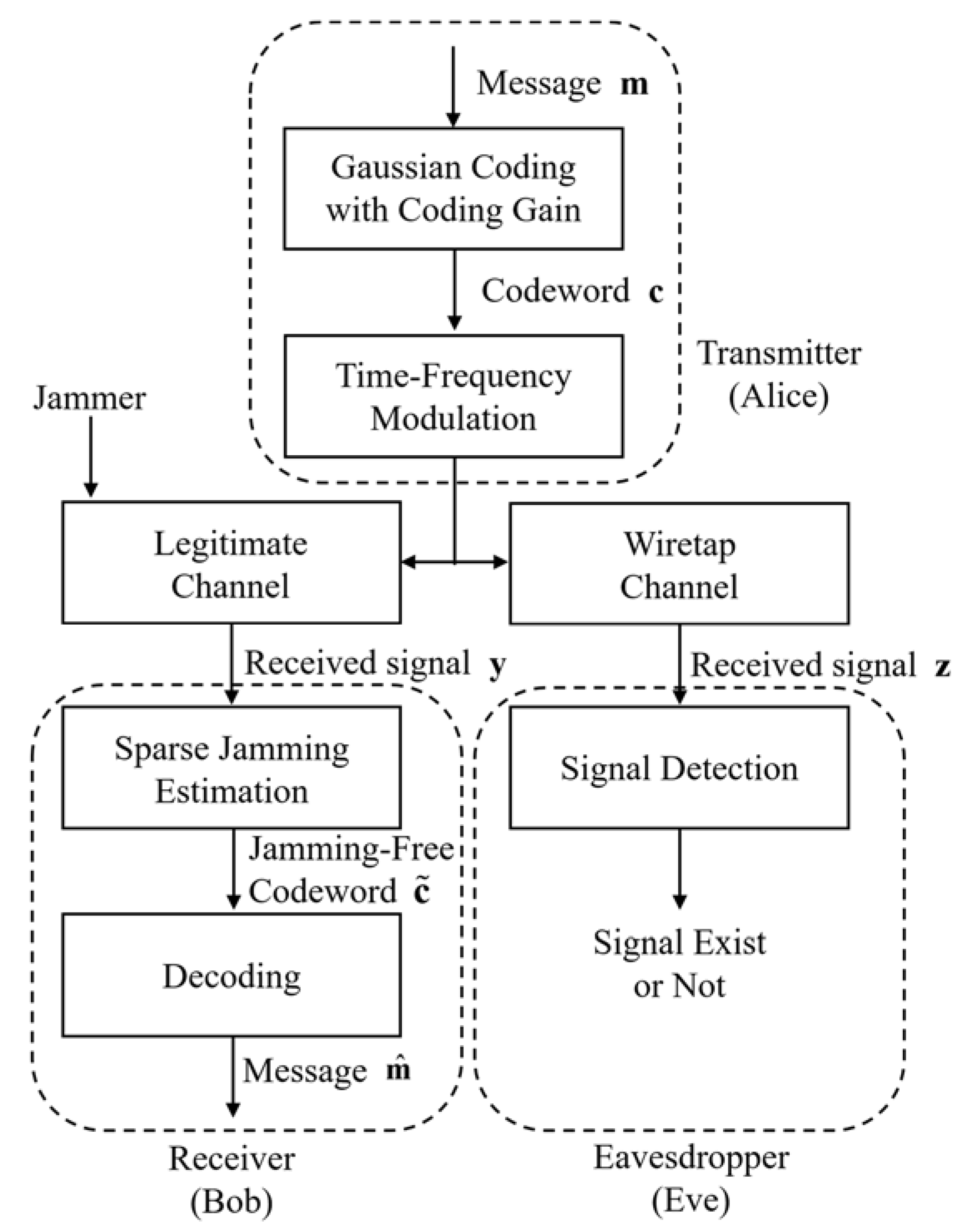
In this paper, we consider wireless communications under a jammer and eavesdropper scenario, for example, the electronic warfare scenario depicted in Figure 1. The proposed system transmits information messages on a coded Gaussian signal through a wireless channel that is attacked by an eavesdropper, called Eve in this paper, and a jammer. We consider two types of jammers. The first type is a blind jammer, which radiates a partial-band or pulse jamming signal without knowing when or where a target communication signal exists. The second type is a follower jammer, which detects an ongoing communication signal and then radiates a jamming signal to interfere with this ongoing signal. We assume that Eve is not aware of the exact codebook and time-frequency band of the target system. Suppose that there is no secret information shared between the transmitter and the receiver. Then the achievability of covert communication depends entirely on the channel quality difference between the receiver and Eve, which is difficult for communicators to control. Thus, many studies assume that the transmitter and the receiver share some secret information, such as a codebook [2,12] or spreading sequence [13,14]. This secret information is often time-varying to prevent information leakage [15]. One practical example is a frequency-hopping radio that exploits the exact time-frequency band of a signal as secret information.

In this paper, we propose a novel covert anti-jamming communication system based on a noise-like Gaussian-coded time-frequency modulation, as illustrated in Figure 2. To provide covertness to a communication signal, we propose a time-frequency modulation scheme. It is difficult to distinguish a signal generated using the proposed scheme from Gaussian noise. To provide robust anti-jamming performance, we propose two receiver algorithms that estimate and remove the jamming signal from the received signal by exploiting the sparse nature of the jamming signal.

The main contributions of this paper are as follows:

• We propose a covert anti-jamming communication system based on Gaussian-coded time-frequency modulation. We consider the communication system that is exposed to the threat of the jammer and Eve. Previous studies on analog coding [5,6,7,9,10,11] have not considered the threat of jammers and eavesdroppers simultaneously. We designed a coding and modulation method for a transmitter to achieve anti-jamming and covert communication simultaneously. For a receiver, to estimate and remove jamming, we propose two novel sparse jamming estimation (SJE) algorithms, i.e., greedy SJE (GSJE) and Bayesian SJE (BSJE), which are described as Algorithm 1 and Algorithm 2, respectively.
• For the proposed Gaussian coding scheme, we aimed to develop a real-valued coding scheme in which a coding gain is provided. Previous studies on analog coding [5,7] have considered analog messages. In this paper, we show that the coding method cannot provide a coding gain for finite-field messages. As a countermeasure, we introduce two methods to achieve coding gain even when the finite-field messages are encoded. The first method is a two-stage coding approach, applying finite-field coding and linear Gaussian coding sequentially. In this method, the overall coding gain is equivalent to that of the finite-field coding used in the first stage. Another coding method is a codebook method that uses a pregenerated codebook rather than a linear operation on message vectors. We demonstrate the existence of a coding gain through numerical results that compare the bit error rate (BER) performance of the proposed system under jamming and the uncoded direct-sequence spread spectrum (DSSS) without jamming.
• We show the undetectability of the signal transmitted from the proposed system. The signal of the proposed system is compared to that of a conventional binary phase-shift keying (BPSK)-DSSS scheme. For this comparison, we considered Eve to be an energy-detecting eavesdropper that can distinguish the communication signal from noise using the maximum likelihood (ML) method. The detection capability of Eve increases as the signal-to-noise ratio (SNR) and false alarm probability increases. Our results demonstrate that the proposed system offers significantly better undetectability than the BPSK-DSSS scheme in such critical cases. Thus, the proposed method is superior when Eve is the most threatening.

The remainder of this paper is organized as follows. In Section 2, Section 3 and Section 4, we describe the proposed covert anti-jamming communication system as depicted in Figure 2. Specifically, we discuss the signal design required to achieve covertness and anti-jamming performance in Section 2. In Section 3, we describe the time-frequency modulation method. In Section 4, we present an analysis of the undetectability of the proposed system and compare it with that of a conventional binary system. Section 5 discusses issues related to implementation, such as modulation methods and computational complexity. In Section 6, we numerically evaluate the BER performance of the proposed system. Finally, Section 7 summarizes our results and concludes the paper.

2. Signal Design

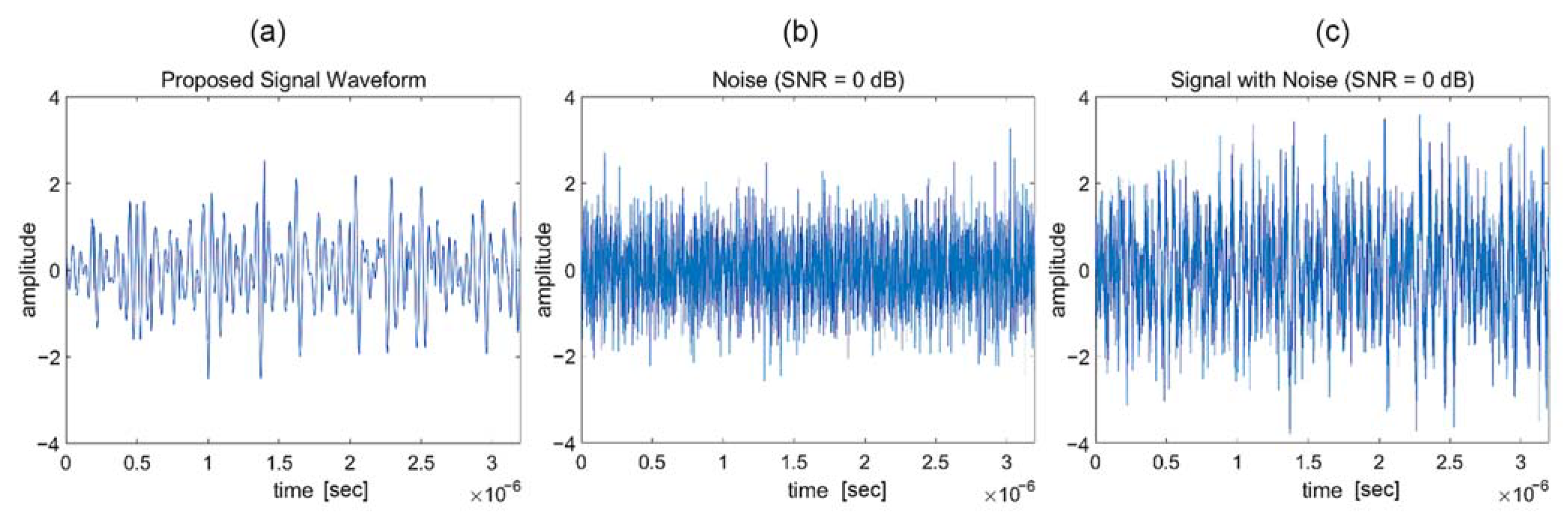
In this section, we describe the proposed signal design. In the proposed system, the codeword alphabet consists of Gaussian-distributed real numbers rather than a finite-field alphabet. The transmitted Gaussian codeword appears as additive white Gaussian noise (AWGN) to Eve. In contrast, the receiver who knows the exact codebook can detect the transmitted codeword even with a significantly low SNR setting. Figure 3a illustrates the time-domain signal waveform of the proposed system at the 0 dB SNR setting. The waveform with noise in Figure 3c is hardly distinguishable from the AWGN in Figure 3b. A detailed analysis of this undetectability is presented in Section 4. In this section, we consider two encoding methods used to construct such codewords. We first introduce the simplest method, linear block coding (LBC), as proposed in previous studies [5,7]. Then, we present the limitations of that method and propose two methods to address these limitations.

2.1. Codeword Generation

A binary message vector $m\in {\{-1,1\}}^L$ is encoded into a real-valued codeword vector $c\in {\mathbb{R}}^{2N}$, where $\mathbb{R}$ is the set of real numbers. Each element of the codeword, i.e., each time-frequency symbol, follows a Gaussian distribution. Here, the encoding $\mathrm{Enc}:{\{-1,1\}}^L\mapsto {\mathbb{R}}^{2N}$ can be any function that includes a redundancy to the codeword. The redundancy can be exploited to estimate the jamming and correct the channel-induced errors.

In the previous work of Candes and Tao [7], LBC-like encoding of the real-valued message was studied. That is, ${\mathrm{Enc}}_{\mathrm{LBC}}:{\mathbb{R}}^L\mapsto {\mathbb{R}}^{2N}$ was previously investigated. As it is a simple method, we can use it as a codeword generation method. We call this method Gaussian-LBC. Let us define the probability density function (PDF) for a Gaussian random variable with a mean $\mu$ and variance ${\sigma }^2$ as $\mathcal{N}(\mu ,{\sigma }^2)$. In the Gaussian-LBC, a codeword vector becomes the product of a generator matrix and a message vector:

$$c=Gm,$$

(1)

where $m$ is the $L$-dimensional message vector, $G\in {\mathbb{R}}^{2N\times L}$ is the generator matrix of which the entries follow $\mathcal{N}(0,1/N)$, and $c\in {\mathbb{R}}^{2N}$ is the codeword vector. Because the method is similar to LBC in finite fields, one can define concepts and notations corresponding to the parity-check matrix, syndromes, and error correction. However, error correction using syndromes in real-valued code is a nonlinear pattern recognition problem that has no simple solution for an arbitrary $G$ [5]. A linear programming solution to this real-valued syndrome decoding problem was described in [7]. The solution has been widely accepted for several other sparse signal recovery (SSR) problems, under the name of CS [8]. Numerous algorithms have been proposed [16,17,18,19] to achieve this solution.

However, we require another approach with Gaussain-LBC. This is because ${\mathrm{Enc}}_{\mathrm{LBC}}$ cannot fully exploit the characteristics of the digital message; thus, one cannot obtain an adequate coding gain. In the following Section 2.2., we discuss an alternate design of $\mathrm{Enc}:{\{-1,1\}}^L\mapsto {\mathbb{R}}^{2N}$ to obtain the coding gain.

2.2. Gaussian Coding with Coding Gain

The Gaussian-LBC method has a limitation in that the method considers only the real-valued message case. However, for modern communication systems that transmit a variety of finite-field messages, the encoding of a finite-field message must be considered. Unfortunately, the direct application of the Gaussian-LBC method to finite-field messages is inefficient because there is no actual coding gain. In finite-field coding, the coding gain is defined by how much the minimum Hamming distance between two codeword vectors increases when compared to that between message vectors. This is because the finite-field decoder maps the input vectors to the closest codeword in terms of the Hamming distance. In contrast, the coding gain of a real-valued code cannot be defined by the Hamming distance because the closeness of real-valued codewords to non-sparse noise is meaningless. Instead, the Euclidean distance has to be used for real-valued code. It can be noted that the minimum Euclidean distance is constant before and after the Gaussian-LBC, i.e.,

$$\begin{array}{cc}\hfill {(c-\tilde{c})}^T(c-\tilde{c})& ={(Gm-G\tilde{m})}^T(Gm-G\tilde{m})\hfill \\ & ={(m-\tilde{m})}^T{G}^{T}G(m-\tilde{m})\hfill \\ & ={(m-\tilde{m})}^T(m-\tilde{m}),\hfill \end{array}$$

(2)

where ${(\cdot )}^T$ is the transpose operator for the vector/matrix and $G^{T}G=I$ for large $N$. To benefit from coding gain, we considered two approaches: concatenation coding and the codebook method.

2.2.1. Concatenation Coding

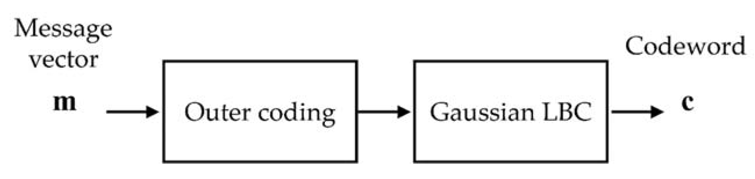
To provide an encoding method with coding gain, concatenation coding was considered. Namely, the encoding of a digital message $\mathrm{Enc}:{\{-1,1\}}^L\mapsto {\mathbb{R}}^{2N}$ becomes a serial combination of two different coding methods, as depicted in Figure 4. The message is encoded twice, first by an outer code ${\mathrm{Enc}}_{out}:{\{-1,1\}}^L\mapsto {\{-1,1\}}^{N_{out}}$ and then by an inner code ${\mathrm{Enc}}_{in}:{\{-1,1\}}^{N_{out}}\mapsto {\mathbb{R}}^{2N}$. We used a finite-field coding method, which yields a coding gain, as the outer code, and then used the Gaussian-LBC as the inner code so that the system could obtain the advantages of both the error-correcting coding and Gaussianity of the signal.

The decoding procedure is also two-fold. Given a jamming-mitigated codeword $\tilde{c}$, the Gaussian-LBC codeword is decoded first by ${\mathrm{Dec}}_{in}:{\mathbb{R}}^{2N}\mapsto {\{-1,1\}}^{N_{out}}$; then, the outer codeword is decoded by ${\mathrm{Dec}}_{out}:{\{-1,1\}}^{N_{out}}\mapsto {\{-1,1\}}^L$. Here, we focus on the decoding of the Gaussian-LBC ${\mathrm{Dec}}_{in}$. Because the decoding of the Gaussian-LBC is equivalent to an overdetermined linear inverse problem (LIP), ML decoding can be performed using the least-squares method with $O(N\cdot N_{out})$ computations, where $N_{out}$ is the length of the outer codeword. If the code rate of the outer code is fixed (i.e., $O(N_{out})=O(L)$), the complexity is equivalent to $O(NL)$. Based on the output of the Gaussian-LBC decoder ${\mathrm{Dec}}_{in}$, the original message is decoded using the outer code decoder ${\mathrm{Dec}}_{out}$, i.e., the recovered message vector $\widehat{m}:={\mathrm{Dec}}_{out}({\mathrm{Dec}}_{in}(\tilde{c}))$.

2.2.2. Gaussian Codebook

The Gaussian codebook method is another coding method with coding gain. If the length of the binary message vector is $L$, then $2^L$ codeword vectors of length $2N$ are pregenerated. Then, the one-by-one mapping encoding function $\mathrm{Enc}:{\{-1,1\}}^L\mapsto {\mathbb{R}}^{2N}$ can be constructed between $2^L$ message vectors and codeword vectors. The codeword can be decoded using the ML method. $O(N{2}^L)$ computations are required to decode the original message from the proposed codeword generated by $\mathrm{Enc}$. Here, we construct a codebook $G$ with a Toeplitz matrix of which the columns are cyclic shifts of a Gaussian random vector $g={[g_1,g_2,\dots ,g_{2N}]}^T$, rather than generating every element of $G$ with an independent and identically distributed (i.i.d.) Gaussian. There are two benefits to constructing the codebook as a Toeplitz matrix. First, the Toeplitz structure accelerates the computation of the decoding method by using the fast Fourier transform (FFT). Second, such a codebook can be stored in a more memory-efficient manner than a random codebook because the Toeplitz codebook requires as much memory space as $O(N)$, whereas the i.i.d. codebook requires as much memory space as $O(N{2}^L)$. If the computational costs of the FFT and inverse FFT (IFFT) are considered, the overall computational complexity becomes $O(N\log N)$.

The concatenation method presented in Section 2.2.1 is attractive in practice because well-studied finite-field coding methods can be directly exploited as the outer code. A proper outer code can be selected according to the purpose and requirements of the system. We used the codebook method in the following simulation section because the Toeplitz codebook method provides a good restricted isometric property (RIP) condition and is independent of the outer code design.

3. System Model

The codewords are transmitted by spreading over a wide block of time-frequency OFDM slots. After demodulation and demultiplexing, the receiver obtains the codewords that are distorted by noise and jamming. The jamming portion is removed using the SSR technique [8]. The receiver decodes the original messages based on the jamming-free codewords.

3.1. Time-Frequency Modulation

The real-valued codeword $c$ of dimension $2N$ can be rewritten as a complex-valued codeword vector of dimension $N$, i.e., $x\in {\mathbb{C}}^N$, where $\mathbb{C}$ is a set of complex numbers. The real part of $x$ is the first half of the vector $c$ and the imaginary part of $x$ is the latter half of $c$. That is, for the real-valued codeword $c={\left[c_1,c_2,\dots ,c_{2N}\right]}^T$, the corresponding complex expression is $x={[c_1+j{c}_{N+1},\dots ,c_N+j{c}_{2N}]}^T$. Each element of $x$ is assigned to the time-frequency grid for transmission by OFDM. Let the number of OFDM subbands be $N_F$ and the number of time slots be $N_T$, where $N=N_F{N}_T$. Figure 5a illustrates the proposed signal in the time-frequency domain, where $N_F=N_T=16$. The signal is transmitted through all 16 subbands, whereas the frequency-hopping spread spectrum (FHSS) signal in Figure 5b uses only a single subband in a time slot. The energy of the proposed signal remains under the noise floor at the plane where the energy = 1, whereas the energy of the FHSS signal with the same power has peaks above the noise floor.

The complex codeword vector $x$ is divided into $N_T$ column vectors, i.e., $x_k$ $(k=1,2,\dots ,N_T)$, where $x={[\begin{array}{cccc}{x}_1^T& x_2^T& \cdots & x_{N_T}^T\end{array}]}^T$. The kth OFDM symbol is determined by an IFFT of $x_k$. Here, we omit the cyclic prefix (CP) for simplicity, as channel estimation and the inter-symbol interference problem are beyond the scope of this paper. If one assumes perfect channel estimation, then the CP being jammed cannot be a problem as the CP is discarded on the receiver side. However, note that jamming attacks on the CP can distort the OFDM system efficiently [20,21], thus degrading the performance of the system. Future research should study the effect of CP jamming.

3.2. Channel Model

There are two separate channels in the proposed system. One is the legitimate channel from the transmitter, Alice, to the legitimate receiver, Bob. The other is a wiretap channel from Alice to the eavesdropper Eve, who is not a legitimate user. We consider that the legitimate channel suffers from hostile jamming, whereas the wiretap channel does not. Figure 6 illustrates the channel model. Bob obtains the signal through the legitimate channel, which is contaminated by jamming, whereas Eve receives the signal through the wiretap channel. This modeling encompasses the following two scenarios within a single logically equivalent scheme. The first scenario is that Eve and the jammer are combined into a single actor. The follower jammer is an example. The second scenario is that the two are located apart. For example, the jammer can be located close to the receiver, whereas the eavesdropper can be placed near the transmitter for better performance. In addition, Alice and Bob share a codebook $\mathcal{C}\in {\mathbb{C}}^N$ which is the set of possible codewords. To focus on covert communication, we assume that Eve does not have the codebook.

Let $h_k$ be the channel impulse response vector of which the length is $N_F$. The kth received vector after OFDM demultiplexing and CP removal is

$$y_k=H_k{x}_k+e_k+w_k,$$

(3)

where $e_k\in {\mathbb{C}}^{N_F}$ is a jamming vector, $w_k\in {\mathbb{C}}^{N_F}$ is additive circularly symmetric complex Gaussian (CSCG) noise, and $H_k\in {\mathbb{C}}^{N_F\times N_F}$ is a diagonal matrix of which the diagonal elements are the FFT of $h_k$. Assuming that the fading channel has no null, the matrix $H_k$ is invertible. The $N_T$ OFDM symbols can be expressed as a single-vector expression through concatenation; as is the case with $x={[\begin{array}{cccc}{x}_1^T& x_2^T& \cdots & x_{N_T}^T\end{array}]}^T$, the single-vector expression for the entire received vector $y={[\begin{array}{cccc}{y}_1^T& y_2^T& \cdots & y_{N_T}^T\end{array}]}^T$ becomes

$$y=Hx+e+w,$$

(4)

where the combined channel matrix $H$ is the block-diagonal matrix consisting of $H_1,H_2,\dots ,H_{N_T}$, $e={[\begin{array}{cccc}{e}_1^T& e_2^T& \cdots & e_{N_T}^T\end{array}]}^T$ is the jamming vector, and $w={[\begin{array}{cccc}{w}_1^T& w_2^T& \cdots & w_{N_T}^T\end{array}]}^T$ is the CSCG noise vector.

3.3. Sparse Jamming Model

In our scenario, the jamming vector $e$ is assumed as a spare vector because practical jammers are modeled as band-limited or time-limited jammers. In fact, a jamming method that interferes with every time-frequency symbol simultaneously would be a powerful jamming method. However, in the proposed covert communication system, the jammer cannot be sure of the exact time-frequency band of the target signal because the proposed system is intended to provide undetectable characteristics of the transmitted waveform, as shown in Section 4. Several studies on the energy optimization of jammers, including [22,23], have indicated that a jamming policy without a precise signal power estimation is not optimal. To achieve energy efficiency, the jammer must acquire the time-frequency band of the target communication.

Without knowing the codebook and exact time-frequency band of target signals, the jammer can have two options—blind barrage jamming and sparse jamming. On the one hand, we consider a barrage jammer that aims to attack a target signal with its signal bandwidth when the time duration is unknown. The jammer cannot launch an attack with a wider bandwidth and longer time duration than those of the target communication signal. Consider $B$ as the bandwidth of the target signal and $D$ as the time duration of the target signal. Obviously, the bandwidth and time duration of the attack signal become $B+\Delta B$ and $D+\Delta D$ for $\Delta B\ge 0$ and $\Delta D\ge 0$, respectively. Here, it can be observed that the jammer would expend an excessive amount of energy due to the amount of excessive time and bandwidth $O(\Delta B\Delta D)$. Nevertheless, the attack by the jammer may still remain ineffective, provided that the time and frequency band of the target signal is unknown. The only option that the barrage jammer has is to spread jamming power over a wide range of time-frequency regions with large $\Delta B$ and $\Delta D$. However, the power budget of a practical jammer is not infinite. Thus, to launch a barrage jamming attack, the energy density per unit time-frequency region shall remain low. In such a case, the effective jamming energy, i.e., the actual jamming energy spent on the target time-frequency region, shall remain small, and the jamming becomes unsuccessful.

On the other hand, the jammer can choose a sparse jamming approach, aiming to reduce the inefficiency of barrage jamming and concentrate the jamming energy onto a specific time-frequency band. Many jammers therefore aim to identify the time-frequency band of the ongoing communications. Once this is identified, an attack can be launched in the form of partial-band noise jamming, such as pulse jamming, as discussed in [9], and reactive jamming, which is discussed in [10]. Thus, the jammers can concentrate their jamming power on a small, selected part of the entire time-frequency band. What does this mean to the proposed covert anti-jamming communication system? The proposed system is supposed to provide undetectable characteristics of the transmitted waveform, which results in two scenarios. On the one hand, jammers cannot detect the presence of the signal or its time-frequency band at all. This is the case when Eve is physically located far from the transmitter. In this case, the jammers do not launch any jamming attacks. On the other hand, in the case in which Eve is close to the transmitter unit, the signal is partially detectable. It can be recalled that our signals are wideband Gaussian signals. Thus, there are a few time-frequency bands of which the energy levels pierce through the noise floor (refer to the illustration in Figure 5). Eve can be deceived that the ongoing communication exists only on those detected time-frequency bands; consequently, Eve will aim to launch precise jamming attacks at the detected time-frequency bands. The previous discussion explains why we have modeled the jamming attacks to be sparse in the time-frequency domain. By exploiting the sparse nature of jamming, Bob can successfully estimate and remove jamming from the received vector.

3.4. Sparse Jamming Estimation

Let us recall the received vector specified in Equation (4). There always exists a nonzero annihilating matrix $A$ such that $AHx=0$, unless $Hx$ spans ${\mathbb{C}}^N$. Let a matrix $G$ be a generator matrix or codebook matrix of which the columns span the range space of the codewords. Here, note that the generator or codebook matrix $G$ is constructed by a random Gaussian distribution, as discussed in Section 2.

Because the codeword space is a subspace of ${\mathbb{C}}^N$, singular-value decomposition (SVD) can be applied to determine the annihilating matrix $A$. Consider an SVD of ${(HG)}^H$, i.e.,

$${(HG)}^H=U\left[\begin{array}{cc}D& 0\end{array}\right]\left[\begin{array}{c}{V}_1^H\\ A\end{array}\right].$$

(5)

It can be determined that $A$ satisfies $AHx=0$ for all possible values of $x$. By multiplying $A$ to both sides of Equation (4), Bob obtains the measurement vector $b$,

$$\begin{array}{cc}\hfill b& =A(e+w)\hfill \\ & =A\tilde{e},\hfill \end{array}$$

(6)

where $\tilde{e}:=e+w$ is the jamming-plus-noise vector. Because $b$ and $A$ are known to Bob, $e$ can be obtained by solving for the SJE problem of Equation (6), which is in the form of a LIP. Unfortunately, the SJE problem is underdetermined because the annihilating matrix $A$ is the null space of $HG$. However, let us recall the assumption that $e$ is a sparse vector. It is known that a sparse vector can be recovered using SSR techniques even if the LIP is underdetermined [7,8,16,17,18,24].

There are two conditions related to the successful reconstruction of the jamming vector $e$ from Equation (6) using SSR techniques. The first condition is that the LIP should have good properties. The goodness of LIP is often measured using a condition referred to as RIP [7] of the sensing matrix. In the proposed SJE problem, the sensing matrix corresponds to the annihilating matrix $A$. Several studies have shown that a sensing matrix has a good RIP if the matrix is created from an i.i.d. zero-mean Gaussian. However, the annihilating matrix $A$ in the SJE problem is not created from such a distribution, but is created from the null space of $HG$.

Several studies have discussed the RIP of the null-space matrix. Candes et al. [7] and Stojnic et al. [25] argued that the null-space matrix of an i.i.d. Gaussian random matrix demonstrates a good property because the null space can consist of an i.i.d. Gaussian random basis. Xu et al. [26] showed that the property of the sensing matrix that is created from the null space of a Toeplitz matrix is good for SSR. Note that $HG$ is a Gaussian matrix because the OFDM channel matrix $H$ is a Gaussian matrix and $G$ is also a Gaussian matrix (refer to Section 2 for more details). Further, $HG$ can be an i.i.d. Gaussian matrix or Gaussian Toeplitz matrix when the channel is a frequency nonselective channel. Thus, these results suggest that the SJE problem can be solved successfully, depending on the channel.

The second condition for successful SSR is that the jamming with noise vector $\tilde{e}$ should be close to the sparse vector. If the energy of a sparse vector is much larger than that of a non-sparse vector, the sum of the two vectors is said to satisfy soft sparsity. Raskutti et al. [27] discussed the convergence of the SSR under the soft sparsity model. Arias-Castro and Eldar [28] studied the premeasurement noise model, which is similar to the soft sparsity model. In their study, it was shown that the premeasurement noise model can be reformulated into a general SSR model (i.e., measurement noise model), with a small cost on RIP. Based on these studies, we can conclude that $\tilde{e}$ can be successfully recovered, as $\tilde{e}$ also satisfies the soft sparsity model. To derive the SJE algorithms, we explored two representative SSR algorithms: greedy algorithms and sparse Bayesian learning (SBL) algorithms. In Section 3.4.1, we propose the GSJE algorithm. In Section 3.4.2., we propose the BSJE algorithm.

3.4.1. Greedy Sparse Jamming Estimation Algorithm

To estimate the sparse jamming vector $e$ from the measurement $b$, one can define a support set $\mathbb{S}\subset \{1,2,\dots ,N\}$, which is a set of indices $k$, such that the $k$th element of $e$ is nonzero. Thus, $\mathbb{S}=\left\{k\right|{\widehat{e}}_k\ne 0,k=1,2,\dots ,N\}$. Let us define $A_{\mathbb{S}}$ and $e_{\mathbb{S}}$ as submatrices/subvectors of which the columns/elements contain atom $a_k$ and coefficient ${\widehat{e}}_k$ for $k\in \mathbb{S}$, respectively. Then, $\widehat{e}$ can be determined by solving the following optimization:

$$\widehat{e}=\underset{e}{\arg \min }{\Vert b-Ae\Vert }^2, \mathrm{subject} \mathrm{to} {\Vert e\Vert }_0\le K,$$

(7)

where $K$ is the maximum number of nonzero coefficients in $e$. Equation (7) is an optimization problem that determines the solution $e$ that minimizes the approximation error with the $l_0$ norm constraint. To solve this problem, several greedy algorithms have been proposed. The greedy algorithms iteratively pursue one column of the annihilating matrix $A$ at a time, which significantly reduces the approximation error. Thus, the estimate of the support set $\mathbb{S}$ grows one by one as the iteration progresses, starting from the empty set in the beginning. The matching pursuit (MP) [29], orthogonal MP (OMP) [18,19] and their variants [30,31] are most relevant to the derivation presented in this Section. The MP algorithm for SSR was first proposed by Mallat and Zhang [29]. By applying the MP algorithm to our problem, we can determine one column of the annihilating matrix $A$ that maximizes the inner product with a residual vector at each iteration, and then calculate the corresponding nonzero coefficient that minimizes the estimation error. Conversely, the OMP algorithm has an additional procedure that updates all the coefficients in the subvector $e_{\mathbb{S}}$ at each iteration using the orthogonal projection of the measurement vector onto the subspace $A_{\mathbb{S}}$.

In this section, we propose the GSJE algorithm, described as Algorithm 1. The algorithm aims to estimate the sparse jamming vector from the received signal vector $y$ in Equation (4). Given $H$, $G$ and $y$, the algorithm calculates $A$ using Equation (5). Then, the jamming vector $e$ is estimated by approximating the solution of Equation (7) using the greedy iteration. We assume that the channel matrix $H$ and codeword space $G$ are known to the receiver. The annihilating matrix $A$ can then be determined from the SVD of ${(HG)}^H$, as given in Equation (5), and used to construct the SJE problem. We assume here that the magnitudes of the nonzero coefficients of the jamming vector $e$ are significantly larger than those of the noise vector $w$, i.e., $\left|\right|e|{|}^2\gg |\left|w\right|{|}^2$. This assumption is called the high jamming-to-noise ratio (JNR) assumption. Under this assumption, each iteration of the GSJE will identify a member of the true support set with high probability. In contrast, if the JNR is significantly low (for example, under −10 dB), the accuracy of SJE under the high JNR assumption might be degraded. However, note that the overall system performance, i.e., BER, is no longer affected by the accuracy of the SJE. However, if JNR is in the moderate region, the failure of the GSJE may cause an overall performance degradation. Thus, the model mismatch becomes more significant in the moderate-JNR region. Another challenge is that the GSJE requires certain prior knowledge about jamming. As discussed above, the parameters $\delta$ and $K$ that determine the termination condition depend on prior information such as sparsity and energy of jamming. We limited the number of maximum iterations by $K$, where the cardinality of the support set is known as $K$. At the same time, we set a lower bound on $\Vert \rho \Vert$ by $\delta$. If the prior knowledge is inexact for determining a proper termination condition, the GSJE might not be able to estimate the exact jamming. The assumption that the receiver has exact prior information a priori might be unrealistic in practice as the jammer and the receiver are adversarial to each other. These effects are of interest in the discussion of our simulation results (refer to Section 6.1).

Algorithm 1 Greedy sparse jamming estimation (GSJE) algorithm

Input: H, G, y, $\delta$, K

Initialize:$A\leftarrow \mathrm{svd}(G^H{H}^H)$, $\rho \leftarrow Ay$, $S\leftarrow \left\{\right\}$

1: do:

2: Find the maximum correlated column index, $k\leftarrow \arg \underset{k\backslash \mathbb{S}}{\max }<a_k,\rho >$

3: Update the support set by storing the index in the support set, $\mathbb{S} \leftarrow \mathbb{S}\cup \left\{k\right\}$

4: Estimate the corresponding coefficient subvector by ${\widehat{e}}_{\mathbb{S}}\leftarrow {(A_{\mathbb{S}}^H{A}_{\mathbb{S}})}^{-1}{A}_{\mathbb{S}}^{H}Ay$

5: Update residual by subtracting the contribution of current support set, $\rho \leftarrow \rho -A\widehat{e}$

6: while $\left|\mathbb{S}\right|\le K$ and $\left|\right|\rho \left|\right|\ge \delta$

return:$\widehat{e}$

3.4.2. Bayesian Spare Jamming Estimation Algorithm

As an alternative to GSJE, we propose a novel BSJE algorithm. In the previous section, we discussed that GSJE requires prior knowledge of jamming, such as the sparsity or power of jamming. Instead, we aim to develop the BSJE method in which the jamming is modeled as a Gaussian mixture and Bayesian inference is sought to estimate the jamming vector. From Equation (6), BSJE determines the posterior estimation of $e$ by exploiting the assumption that $e$ is a realization of a zero-mean i.i.d. Gaussian-distributed random vector of which the covariance matrix is $\Gamma =diag[\begin{array}{cccc}{\gamma }_1& {\gamma }_2& \dots \cdots & {\gamma }_N\end{array}]$ (i.e., $e~\mathcal{C}\mathcal{N}(0,\Gamma )$). A simple suboptimal solution is to determine the maximum a posteriori probability (MAP) estimation without exploiting $\Gamma$, i.e.,

$$\widehat{e}=\arg \underset{e}{\max } p(e|b),$$

(8)

where $p(e|b)$ is a conditional PDF. In contrast, the BSJE algorithm exploits the information about $\Gamma$ by applying SBL [24]. Let the ML estimation of $\Gamma$ be $\widehat{\Gamma }$. The algorithm first determines $\widehat{\Gamma }$ and then evaluates the MAP estimator for a given $\widehat{\Gamma }$. That is,

$$\widehat{e}=\arg \underset{e}{\max } p(e|\widehat{\Gamma })p(\widehat{\Gamma })p(b|e),$$

(9)

where

$$\begin{array}{cc}\hfill \widehat{\Gamma }& =\arg \underset{\Gamma }{\max } p(\Gamma |b)\hfill \\ & =\arg \underset{\Gamma }{\max } p(\Gamma ) p(b|\Gamma )\hfill \\ & =\arg \underset{\Gamma }{\max } p(\Gamma ){\displaystyle \int p(b|e)p(e|\Gamma )de}.\hfill \end{array}$$

(10)

To solve the optimization problem, the spirit of expectation-maximization (EM) is exploited; rather than directly maximizing the log-likelihood, the algorithm maximizes the $Q$ function iteratively. The $Q$ function is defined by

$$Q(\Gamma )=E_{e|b;\gamma }\left[\log p(b|e)+\log p(e|\Gamma )+\log p(\Gamma )\right],$$

(11)

and the solution to Equation (10) is equivalent to the maximizer of Equation (11),

$$\widehat{\Gamma }=\arg \underset{\Gamma }{\max }Q(\Gamma ).$$

(12)

Let us recall the SJE problem in Equation (6). The given problem is a form of the so-called input noise model:

$$b=A(e+w).$$

(13)

The closed-form solution to Equation (12) is well known as

$${\widehat{\gamma }}_k=E_{e|b,{\gamma }_k,{\sigma }^2}|e_k{|}^2, (k=1,2,\dots ,N),$$

(14)

which is a solution to $\partial Q(\Gamma )/\partial {\gamma }_k=0$ by assuming $p({\gamma }_k)=1$ and approximating $Q(\Gamma )$ as

$$Q(\Gamma )\approx E_{e|b;\gamma ,{\sigma }^2}\left[{\displaystyle \sum _k-\frac{1}{2}\log {\gamma }_k-\frac{|e_k{|}^2}{{\gamma }_k}+\log p({\gamma }_k)}\right].$$

(15)

If we assume a CSCG jamming $e~\mathcal{C}\mathcal{N}(0,\Gamma )$ and a CSCG noise $w~\mathcal{C}\mathcal{N}(0,{\sigma }^{2}I)$ with given noise variance ${\sigma }^2$, the conditional PDF $p(e|b;\Gamma ,{\sigma }^2)$ becomes CSCG, with mean vector $\mathsf{\mu }$ and covariance matrix $\Sigma$, where

$$\mathsf{\mu }=\Gamma A^H{(A\Gamma A^H+{\sigma }^{2}A{A}^H)}^{-1}b,$$

(16)

$$\Sigma =\Gamma -\Gamma A^H{(A\Gamma A^H+{\sigma }^{2}A{A}^H)}^{-1}A\Gamma .$$

(17)

Thus, the ML estimator in Equation (12) becomes

$${\widehat{\gamma }}_k={\Sigma }_{kk}+{\left|{\mu }_k\right|}^2,$$

(18)

where ${\mu }_k$ is the $k$th element of $\mu$ and ${\Sigma }_{kk}$ is the $k$th diagonal element of $\Sigma$. According to Equations (16)–(18), $\widehat{\Gamma }$ can be determined by iteratively updating ${\Gamma }^{(t)}$ at the $t$th iteration, and by repeating the iteration until convergence. A little is known about the convergence of EM iteration, including the monotonicity property [32]. This property states that the solution converges to at least a saddle point or local optimum. After $\widehat{\Gamma }$ is converged, the MAP estimation is obtained by

$$\begin{array}{cc}\hfill \widehat{e}& =\arg \underset{e}{\max } p(e|b;\widehat{\Gamma },{\sigma }^2)\hfill \\ & ={\mu }_{e|b}(\widehat{\Gamma })\hfill \\ & =\widehat{\Gamma }{A}^H{(A\widehat{\Gamma }{A}^H+{\sigma }^{2}A{A}^H)}^{-1}b.\hfill \end{array}$$

(19)

It can be recalled that our goal is to determine the complex-valued codeword $x$, not $e$ itself, which is obtained by the iteration above. To estimate, we must determine not only $\widehat{e}$ but also $\widehat{w}$; thus, $\widehat{x}$ can be calculated by

$$\widehat{x}=H^{-1}(\widehat{e}+\widehat{w}).$$

(20)

Here, $\widehat{w}$ can be obtained during the BSJE iteration using the same method used for determining $\widehat{e}$, as $\widehat{w}$ also follows a CSCG distribution such that $\mathcal{C}\mathcal{N}(0,{\sigma }^{2}I)$. The MAP estimation of $w$ can be calculated within the same iteration for determining $\widehat{e}$ in Equation (16):

$$\widehat{w}={\sigma }^2{A}^H{(A\Gamma A^H+{\sigma }^{2}A{A}^H)}^{-1}b.$$

(21)

Note that Equations (16) and (17) are equivalent to the equations presented by Giri and Rao (numbered as Equations (36) and (37), respectively, in their paper) [24] if $A^H$ is orthonormal. This implies that if all codewords are orthonormal with each other and the channel matrix $H$ is an identity matrix (i.e., a frequency-nonselective channel), the proposed BSJE algorithm is equivalent to the SBL algorithm for the general measurement noise model.

The BSJE algorithm for the proposed system is described as Algorithm 2. To guarantee the completeness of the algorithm, two parameters, $t_{\max }$ and $\delta$, can be specified. $t_{\max }$ is defined by the maximum number of iterations and $\delta$ is the lower bound on the minimum required update, $\mathrm{tr}(|{\Gamma }^{(t)}-{\Gamma }^{(t-1)}|)$, where $\mathrm{tr}()$ is the trace operator. These two parameters can be set according to the time budget.

The BSJE algorithm does not require prior knowledge about jamming. The BSJE algorithm only requires the channel, codebook, and noise variance as inputs, which can be easily obtained by a legitimate receiver. This mild requirement on prior information is a potential benefit of BSJE, making it more attractive than GSJE in practical implementation. Furthermore, the BSJE algorithm has no model-mismatch problem in the arbitrary JNR condition region, whereas GSJE suffers from estimation performance degradation in the moderate-JNR region.

Algorithm 2 Bayesian sparse jamming estimation (BSJE) algorithm

Input: H, G, ${\sigma }^2$, $t_{\max }$, $\delta$

Initialize:$A\leftarrow \mathrm{svd}(G^H{H}^H)$, $b\leftarrow Ay$, ${\Gamma }^{(0)}\leftarrow I$

1: for $t=0$ to $t_{\max }$ do:

2: Compute $T$ matrix by $T\leftarrow A^H{(A{\Gamma }^{(t)}{A}^H+{\sigma }^{2}A{A}^H)}^{-1}$

3: Update the mean vector $\mu \leftarrow {\Gamma }^{(t)}Tb$

4: Update the noise vector $w\leftarrow {\sigma }^{2}Tb$

5: Update the covariance matrix $\Sigma \leftarrow {\Gamma }^{(t)}-{\Gamma }^{(t)}TA{\Gamma }^{(t)}$

6: Update the hyperparameter ${\Gamma }^{(t+1)}\leftarrow diag(|{\mu }_k{|}^2+{\Sigma }_{kk}){|}_{k=1,2,\dots ,N}$

7: while $t\le t_{\max }$ and $tr(|{\Gamma }^{(t)}-{\Gamma }^{(t-1)}|)\ge \delta$

return:$\tilde{e}\leftarrow \mu +w$

3.5. Decoding

Using GSJE and BSJE, we can successfully estimate the jamming with a noise vector $\tilde{e}$. Then, Bob can obtain the jamming-mitigated complex-valued codeword $\tilde{x}$ by subtracting the estimation of $\tilde{e}$ from $y$. The corresponding real-valued codeword $\tilde{c}$ is obtained by cascading the real and imaginary parts of $\tilde{x}$. Decoding the original codeword $m$ from $\tilde{c}$ is typically performed using MAP estimation, which is a procedure to obtain the most likely input for a given output, i.e.,

$$\widehat{m}=\arg \underset{m}{\max } p(m;\tilde{c}).$$

(22)

Assuming a message m has a uniform distribution, the MAP estimator is equivalent to the ML estimator [33]. The ML estimator of m is defined by $\widehat{m}$, which maximizes the likelihood function. This relationship is represented as follows:

$$\widehat{m}=\arg \underset{m}{\max } p({\widehat{c}}^{\prime };m).$$

(23)

4. Undetectability Analysis

In this section, we present a comparison of the undetectability of the Gaussian-coded time-frequency modulation and binary modulation methods in terms of detection probability for Eve. To measure undetectability, a privacy rate was proposed in [2]. The privacy rate is defined by the number of bits that can be transmitted covertly through the use of $N$ channels. According to [2], only $O\left(\sqrt{N}\right)$ bits can be transmitted covertly; thus, the privacy rate cannot be a constant. However, [3,34] determined that a constant privacy rate is achievable if Eve is uncertain of the channel noise level. Conversely, detection probability is a simple and useful metric of undetectability. For example, the detection probability of chaotic-sequence DSSS signals was studied in [13,14]. The authors assumed that Eve knows most of the protocols used by target communication systems, such as carrier frequency, modulation, length of the spread sequence, and symbol duration, but not the exact spreading sequence. Then, she can attempt matched filtering with all possible spreading sequences for the received samples to determine if a signal exists. The studies determined the detection probability of chaotic DSSS signals for several types of chaotic sequences and compared the probability with that of conventional binary sequence DSSS signals.

To measure undetectability, we considered the detection probability as a metric. The eavesdropping problem was formulated as a hypothesis test. We explored the problem by dividing it into three cases according to uncertainty of noise for Eve. In the first case, Eve is assumed to have no information on the noise level. That is, Eve has an infinitely large uncertainty in terms of the noise level. In such extreme cases, the only option for Eve is to test whether the received samples are from a white Gaussian distribution or from other random distributions, i.e., Eve aims to determine the existence of a signal using a normality test. The second case is the other extreme scenario on the opposite side. In the second case, Eve has no uncertainty regarding the noise level. Thus, Eve knows the exact noise energy. In such a case, Eve can apply a hypothesis test based on a threshold of the symbol energy to distinguish whether the signal exists or not. However, the two extreme cases rarely occur in practice. Thus, in the third case, we define a parameter $\rho$ to quantify the amount of uncertainty Eve has on the noise level. In the following subsections, we measure and compare the undetectability of the proposed signal and conventional signals.

4.1. Undetectability under an Unknown Noise Level

In the first case, Eve is assumed to have no information on the noise level (Case 1). In the following section, we provide a simple analysis and example showing that Eve cannot distinguish the proposed signal, although she has a chance of detecting conventional signals. Let us recall the channel model depicted in Figure 6 to determine the eavesdropping problem. Using the same vectorizing process as the legitimate channel model as presented in Equations (3) and (4), Eve obtains

$$z=H^{\prime }x+w^{\prime },$$

(24)

where $H^{\prime }$ is a combined wiretap channel matrix and $w^{\prime }$ is a CSCG noise vector, which are derived using the same method as those of a legitimate channel, as discussed in Section 3.2.

Consider that Eve monitors the communication channel and obtains a measurement vector assuming an exact carrier frequency, phase, and symbol duration. Moreover, consider a perfect channel state information and flat fading at Eve, which is a threat scenario for a WCS. Then, the receiving model is simplified to

$$z=h^{\prime }x+w^{\prime },$$

(25)

where $h^{\prime }$ is the channel coefficient satisfying $H^{\prime }=h^{\prime }I$. In this scenario, Eve has to determine whether there is a signal using the hypothesis test:

$$\{\begin{array}{l}{H}_0:d=n\\ H_1:d=c+n,\end{array}$$

(26)

where $c={[\begin{array}{cc}real{(x)}^T& imag{(x)}^T\end{array}]}^T$ is the real-valued codeword of which the entries are zero-mean Gaussian random variables with variance ${\sigma }_c^2$, $n={[\begin{array}{cc}real{(w^{\prime }/h^{\prime })}^T& imag{(w^{\prime }/h^{\prime })}^T\end{array}]}^T$ is the AWGN whose entries are zero-mean Gaussian random variables with variance ${\sigma }_n^2$, and $d={[\begin{array}{cc}real{(z/h^{\prime })}^T& imag{(z/h^{\prime })}^T\end{array}]}^T$ is the channel-compensated measurement vector.

In Case 1, Eve has to determine which hypothesis is true based on the PDF of $d$. Let the variance of $d$ be ${\sigma }_d^2$. To test the two hypotheses, the only thing Eve can do is compare how close the sample distribution is to the distribution of Gaussian noise. This test is well known as the normality test. First, assume that Eve demonstrates perfection while calculating the sample distribution. Perfect here implies that Eve can collect an infinite number of samples each with infinite resolution; thus, the histogram distribution of the perfect Eve is identical to the distribution according to the true hypothesis.

Lemma 1.

Assume that Eve is perfect while calculating the sample distribution. Let Eve not know the noise level. Then, she cannot detect the existence of the proposed signal, but she can detect finite-field modulated signals.

Proof of Lemma 1.

Eve does not know the noise level. The addition of the Gaussian signal sample to the Gaussian noise sample produces a Gaussian sample. Thus, what Eve observes are Gaussian samples; Eve can only treat it as Gaussian noise. When Eve observes finite-level signal samples, a perfect Eve will notice that the observed signal deviates from the Gaussian samples. Thus, Eve can detect the presence of an ongoing communication signal. □

It is worth noting that Lemma 1 is satisfied in the ideal case. Namely, it holds when the degree of freedom of the codebook is infinite and Eve can correct an infinite number of samples. However, both conditions cannot be perfect in practice. The degree of freedom of a fixed codebook is limited by the size of the codebook. It causes a distortion between the distributions of the actual symbol and desired Gaussian symbols. In addition, Eve must perform the normality test with a finite number of samples and a finite level of precision. This means that the error probability of the normality test is not zero even for the Gaussian signal. However, the distortion of the distribution can be compensated for by the limited resolvability [35] of the channel between the transmitter and Eve. Since the channel is noisy, small distortions of the input distribution cannot affect the test output of Eve. Moreover, despite all these limitations, it is obvious that the probability of being detected for the proposed signal is far lower than the probability of any conventional non-Gaussian signal.

4.2. Undetectability under an Exact Noise Level

Now, let us focus on Case 2. In this case, Eve is assumed to have perfect information on the noise level. The simplest solution for this testing strategy is to use an energy detector of which the goal is to determine whether the signal is present by comparing the energy of the received symbol.

In the energy detection, the test statistic of Equation (26) becomes the squared sum of symbols. As we assumed, Eve does not know the exact time-frequency band of the target signals. Then, Eve has two strategies for testing. The first is obtaining a single test statistic by integrating the whole energy over a suspected time-frequency band. It is obvious that the test statistic depends on both the SNR and the suspected region, regardless of the coding and modulation method of the target signal. Then the test result depends only on how accurate the suspected region is. Rather than this trivial case, we focus on the other strategy: dividing the suspected region with as fine a grid as Eve can produce, and applying per-symbol energy detection to determine the signal existence according to each time-frequency slot. By this strategy, Eve can evaluate the slot-by-slot possibility of signal presence. Based on this possibility, Eve can jointly estimate the suspected region and probability of signal presence. The performance of this joint detection of possibility and region depends on the per-symbol test. From this aspect, we derive the true positive of the per-symbol hypothesis test (i.e., probability of detection). We compare the probability for the proposed method and that for the conventional binary method, which follows Lemma 2.

Lemma 2.

Let Eve, using an energy-detecting strategy, know the exact noise level. If Eve has a false alarm probability$P_F$, then the per-symbol detection probabilities of the proposed signal$P_{D,Gaussian}$and BPSK-modulated signal P_D,Binary are

$$\begin{array}{c}{P}_{D,Binary}=Q\left(\alpha -\sqrt{\beta }\right)+Q\left(\alpha +\sqrt{\beta }\right),\hfill \\ P_{D,Gaussian}=2Q\left(\frac{\alpha }{\sqrt{1+\beta }}\right),\hfill \end{array}$$

(27)

where$\alpha =Q^{-1}(P_F/2)/{\sigma }_n$,$\beta ={\sigma }_c^2/{\sigma }_n^2$, andthe$Q$-function is defined by

$$Q(x)=\frac{1}{\sqrt{2\pi }}{\displaystyle {\int }_x^{\infty }{e}^{-t^2/2}dt}.$$

(28)

Proof of Lemma 2.

In Case 2, Eve has information about the wiretap channel noise level. Without the loss of generality, the hypothesis test in Equation (26) is simplified into a per-symbol hypothesis test, as shown below:

$$\{\begin{array}{l}{H^{\prime }}_0:d=n\\ {H^{\prime }}_1:d=c+n,\end{array}$$

(29)

where $d$, $c$, and $n$ are the corresponding single samples of $d$, $c$, and $n$. We determine a threshold $\alpha$ and use the following likelihood ratio test to determine which hypothesis is true:

(30)

The threshold $\alpha$ is selected according to the desired false alarm probability $P_F$. Because the noise is Gaussian, $\alpha$ can be calculated using the $Q$-function:

$$\alpha =Q^{-1}\left(\frac{P_F}{2}\right).$$

(31)

We can now compare the probability of detection for the traditional binary modulation and proposed modulation methods. The probability of detection can be calculated as the $\alpha {\sigma }_n$-tail probability of the distribution of $d$ given that ${H^{\prime }}_1$ is true, through a process similar to that used in [13,14]. For a binary modulation scheme of which the constellation is distributed uniformly at the points $\pm {\sigma }_c$, the distribution of $d$ when ${H^{\prime }}_1$ is true becomes

$$f_b(x)=\frac{1}{2\sqrt{2\pi {\sigma }_n^2}}{e}^{-\frac{{(x-{\sigma }_c)}^2}{2{\sigma }_n^2}}+\frac{1}{2\sqrt{2\pi {\sigma }_n^2}}{e}^{-\frac{{(x+{\sigma }_c)}^2}{2{\sigma }_n^2}}.$$

(32)

The probability of detection for a uniformly distributed binary signal is

$$P_{D,Binary}=Q\left(\frac{\alpha {\sigma }_n-{\sigma }_c}{{\sigma }_n}\right)+Q\left(\frac{\alpha {\sigma }_n+{\sigma }_c}{{\sigma }_n}\right).$$

(33)

In contrast, consider the proposed signal of which the sample value obeys a Gaussian random distribution with zero mean and variance ${\sigma }_c^2$. Then, the PDF of $(d|{H^{\prime }}_1)$ is also a Gaussian PDF with zero mean and ${\sigma }_c^2+{\sigma }_n^2$ variance. The $\alpha$-tail probability is calculated directly as

$$P_{D,Gaussian}=2Q\left(\frac{\alpha {\sigma }_n}{\sqrt{{\sigma }_n^2+{\sigma }_c^2}}\right).$$

(34)

Letting $\beta ={\sigma }_c^2/{\sigma }_n^2$, the two probabilities obtained using Equations (33) and (34) are equivalent to Equation (27). □

Lemma 2 shows that if the normalized SNR of Eve is $\beta <<1$, the two probabilities are nearly identical. In contrast, if $\beta \to \infty$, the detection probability of a Gaussian signal is lower than that of a binary signal. Thus, if the SNR of the channel between Alice and Eve is higher, a Gaussian signal is superior to a binary signal in terms of undetectability.

At a moderate SNR, the false alarm probability of Eve (parameter $\alpha$) determines the detection probability. As the false alarm probability increases (i.e., Eve is more sensitive), a Gaussian symbol becomes more undetectable than a binary symbol.

4.3. Undetectability under an Uncertain Noise Level

In practice, Eve must estimate the noise level, ${\sigma }_n^2$, to determine the proper threshold, $\alpha$. The estimation error affects the tradeoff between the detection probability and the false alarm probability. Let the estimated noise variance be ${\sigma }_{est}^2:=\rho {\sigma }_n^2$ using an uncertainty parameter, $\rho \in \left[{\rho }_{\min },{\rho }_{\max }\right]$. Under this definition, the uncertainty increases when the interval $\left[{\rho }_{\min },{\rho }_{\max }\right]$ grows. In contrast, the uncertainty becomes smaller when the interval becomes narrower, and finally becomes zero when ${\rho }_{\min }={\rho }_{\max }=1$. In this scenario, Eve sets the parameter $\alpha$ by using ${\sigma }_{est}^2$ instead of ${\sigma }_n^2$ to set the decision threshold, $\alpha {\sigma }_{est}$. Then, the detection and false alarm probabilities in Lemma 2 change according to $\rho$, as shown below.

Lemma 3.

Let Eve, using an energy-detecting strategy, estimate the noise level to be${\sigma }_{est}^2:=\rho {\sigma }_n^2$with the uncertainty parameter$\rho$. Then, for the target false alarm probability of Eve,$P_{F,\mathrm{target}}=2Q(\alpha )$, the per-symbol detection probabilities of the proposed signal$P_{D,Gaussian}$and BPSK-modulated signal P_D,Binary are

$$\begin{array}{c}{P}_{D,Binary}=Q\left(\alpha \sqrt{\rho }-\sqrt{\beta }\right)+Q\left(\alpha \sqrt{\rho }+\sqrt{\beta }\right),\hfill \\ P_{D,Gaussian}=2Q\left(\frac{\alpha \sqrt{\rho }}{\sqrt{1+\beta }}\right),\hfill \end{array}$$

(35)

and the actual false alarm probability becomes$P_F=2Q(\alpha \sqrt{\rho })$.

One can easily prove Lemma 3 by calculating the $\alpha {\sigma }_{est}$-tail probability using the same procedure as used in Equations (32)–(34). Lemma 3 shows that the uncertainty of the noise level of Eve only causes a shift in the tradeoff between the detection probability and the false alarm probability. This implies that $P_F$ increases and $P_D$ decreases if Eve underestimates ($\rho <1$) the noise level; in contrast, $P_F$ decreases and $P_D$ increases if Eve overestimates ($\rho >1$) the noise level. The results for different $\rho$ are illustrated in Figure 7.

In conclusion, Lemma 1 shows that the proposed method is more undetectable than the finite-field modulation method, regardless of the eavesdropping scenario. Lemmas 2 and 3 show that the proposed method is more undetectable than the traditional binary modulation method, especially when the eavesdropping scenario is more threatening.

5. Implementation Problems

Showing how the proposed system is implemented in real time is important. In this section, we aim to present two problems in real-time implementation and address solutions for each. The first is modulation. The proposed system achieves undetectability from Gaussian-distributed codeword samples. However, digital signal processing units do not usually support Gaussian samples. Therefore, in Section 5.1, we discuss how the Gaussian samples can be represented with finite precision, and determine the number of quantization levels required for sufficient precision. The possible adoption of commercially applicable solutions such as analog-to-digital converters and digital signal processing units are discussed as well in order to tackle this finite precision problem. The second problem is computational complexity. The SSR algorithms include the matrix inversion operation in each iteration. In Section 5.2, we aim to show that hardware/software solutions such as parallel processing, field-programmable gate array (FPGAs), and application-specific integrated circuits (ASICs) can achieve high throughput and satisfy power constraints.

5.1. Modulation Method

In our proposed system, we used Gaussian samples. This has a noise-mimicking property that is highly likely to remain undetected by the watchful Eve. This undetectable characteristic of the Gaussian code is bolstered with the time-frequency modulation, which is not available with traditional digital modulation constellations, such as quadrature phase-shift keying (QPSK) and quadrature amplitude modulation (QAM). We can recall that in Section 4, the proposed method showed higher undetectability than the traditional method, especially in the scenario in which Eve is the most threatening.

The proposed system has to be implemented in signal processing processors that have a finite dynamic range and a finite number of precision levels. Hence, truncation and quantization must be considered when implementing the Gaussian constellation. For several decades, optimal quantization methods have been studied in signal processing and machine learning communities. Well-known quantization methods include Lloyd’s algorithm I [36]. It determines a partition with respect to k mean points or quantization points and then updates these points by calculating the center of each partition. Generalized vector quantization [37] is a relaxation of Lloyd’s algorithm. It combines Lloyd’s algorithm with a global optimization method to avoid local minimums. There are several other heuristic algorithms for determining optimal quantization, such as competitive learning vector quantization [38].

The most important parameter for these methods is the number of quantization points, which determines the truncation limits and quantization precision. If the number of quantization points is large, the undetectability performance of the quantized Gaussian signal becomes closer to that of an ideal Gaussian signal. As the number of quantization points increases, a more precise analog-to-digital converter is required.

The quantized Gaussian constellation methods allow us to transmit and receive an approximation of the proposed Gaussian-coded signal by bounding the maximum magnitude with finite values. For example, Pages and Printems [38] designed a 500-point quantized constellation that closely approximates the ideal Gaussian signal. For this constellation, the maximum magnitude of a sample is bounded by $3\sqrt{E_s}$, where $E_s$ is the average energy of the signal constellation. This result shows that the proposed method with quantization can be achieved in modern radios. For example, the commercial mobile radio platform of Qualcomm, called Snapdragon 855, includes a long-term evolution modem that supports 256-QAM [39]. When 256-QAM is used, the maximum magnitude of a sample is bounded by $1.6\sqrt{E_s}$. Thus, the dynamic range required for a quantized Gaussian constellation is not significantly far from the dynamic range of the specifications of commercial hardware.

If the quantized Gaussian signal is used instead of the true Gaussian signal, performance degradation might occur due to the gap between the two distributions. However, the difference will be negligible if the quantization precision is sufficiently high. In

Table 1. Average results of the Anderson–Darling test for quantized Gaussian distribution.

Quantization Level [bits]	16	14	12	10	8
Average Return	0.0557	0.0583	0.0624	0.0661	0.1969

, the results of the Anderson–Darling test for samples from a quantized and truncated Gaussian distribution are listed. If the quantized Gaussian distribution is close to the real Gaussian distribution, the test returns 0; otherwise, it returns 1. In the numerical simulation, 1024 realizations of 8-, 10-, 12-, 14-, and 16-bit quantized distributions were considered; moreover, a [–3, 3]-truncated standard normal distribution was tested. The results of the tests were averaged from 10,000 simulations per simulation point. The results show that with a significance level of 5%, the probability of distinguishing between the samples from 12-bit quantization and the samples from the true Gaussian distribution is as small as 6.24%. It can be noted that a $1000 software-defined radio device includes a 12-bit digital-to-analog converter [40]. Thus, we can conclude that the quantized Gaussian signal is sufficiently close to the real Gaussian signal despite the hardware limitation.

5.2. Computational Complexity and Power Consumption

The computational complexity is another important consideration for real-time implementation. The receivers of the proposed system include the SSR algorithm for solving the SJE problem and removing it from the received vector. The additional computation of the SSR algorithm requires a certain amount of processing time and power consumption. On the one hand, for the GSJE algorithm, the dominant complexity term is that of the least-squares method for obtaining nonzero coefficients. The computational complexity of the least-squares or the equivalent matrix inversion method is $O(NK)$ per iteration, because the Cholesky decomposition of $A_{\mathbb{S}}^H{A}_{\mathbb{S}}$ can be precalculated for all possible support sets, $\mathbb{S}$. The amount of overall computations for $K$ number of iterations is $O(N{K}^2)$. Conversely, the BSJE algorithm has to calculate an inversion of the matrix ${(A\Gamma A^H+{\sigma }^{2}A{A}^H)}^{-1}$ for each iteration, resulting in $O(MN)$ computations, where $A\in {\mathbb{C}}^{M\times N}$ and $M<N$. We now discuss the complexity of two other conventional covert anti-jamming methods. The simplest conventional method is the DSSS, which is compared with the proposed method in Section 4. The receiver for DSSS requires $O(N)$ computations to perform a matched filtering of length $2N$. The other conventional method, FHSS-type cognitive radio [41,42], also requires $O(N)$ computations for spectrum sensing of $N_F$ subbands within $O(N_T)$ hops. The results show that the complexity of the SSR algorithm is marginally higher than that of these conventional methods. However, owing to the recent advances in software and hardware solutions, this complexity increase does not pose any limitation to real-time implementation. We aim to show this in the following section.

Let the block size be $N=2^9$ for transmitting a message of length $l_m=16$. Then, the computational complexity of the GSJE algorithm is approximately $2^{23}\approx 8\times {10}^6$ floating-point operations per second (FLOPS), assuming the worst case where $K=N/4$. We can use serial processing with modern digital signal processing chips to compute the algorithm. For example, a single core of the TMS320C6678 digital signal processor offers a few tens of giga-FLOPS. When we employ these chips, we can process a few thousand blocks in real time, while consuming 1 W [43]. This implies that the throughput that the proposed transceiver offers can easily support communication speeds on the order of kilobits per second(kbps), while offering covert communication with strong anti-jamming protection.

We can increase the speed of the SSR algorithm. To achieve this, we can utilize recent advances in research on parallel computation for matrix inversion and multithread processing on GPUs. Examples include Gauss–Jordan-based implementations [44] and squared Givens rotation-based implementations [45]. Sharma et al. [44] claimed that the time complexity of the matrix inversion decreased up to $O(N)$ and Yu et al. [45] showed that their CPU/GPU-combined implementations achieved more than 20 times higher throughput than CPU-only implementations. These examples suggest the possibility of a real-time implementation on the order of megabits per second based on a GPU or a cluster of GPUs. However, the challenge of power consumption remains. For example, the GPU cores used in [45] consume a maximum of 49 W. These additional power requirements might not be bearable for certain power-critical applications, such as a mobile radio device.

To satisfy the power constraints of real-time applications, hardware solutions such as FPGAs and ASICs can be utilized. FPGA implementations [46,47] can process the SSR algorithm sufficiently fast, within the order of 10 μs. The implementations in [46,47] run the SSR algorithm for $N=128$ within 18.3 μs and 27.0 μs, respectively. If we assume $N=128$ and $L=4$, the throughputs of the implementations become 218.6 and 148.1 kbps, respectively. ASICs can be used to further increase the throughput. A 65-nm complementary metal-oxide-semiconductor ASIC design [48] can process the GSJE algorithm for $N=256$ within 591.36 ns. By assuming $N=256$ and $L=8$, a throughput of 13.53 Mbps can be achieved.

It may appear that adding an ASIC for the sole purpose of eliminating jamming is too expensive. However, it must be noted that hardware costs decrease rapidly each year. Furthermore, it should be noted that achieving covert communication capability with anti-jamming protection in any battlefield situation is highly desired. Imagine a situation in which the entire communication link between allied forces is disabled and destroyed by hostile jamming. Multiple studies emphasize how detrimental it is to have even a minor information loss in mission-critical military communications [49,50].

6. Results

In this section, we present numerical results to demonstrate the anti-jamming performance of the proposed system. First, we compare the SJE qualities of the two algorithms, GSJE and BSJE, in terms of the mean squared error (MSE). Second, we demonstrate the BER at the receiver under a jamming attack using several channels (AWGN and frequency-selective fading), coding methods (linear Gaussian and codebook), and jamming estimation algorithms (GSJE and BSJE).

6.1. Sparse Jamming Estimation Error

We evaluated the SJE performance of the GSJE and BSJE algorithms for the proposed system. In general, the BSJE algorithm shows better SJE performance than the GSJE. However, as the two algorithms have advantages and disadvantages, we must select an algorithm for practical applications.

• Limitations in BSJE implementation

In practical implementations, the appropriate maximum number of iterations should be chosen to ensure the completeness of the iterative algorithm. As the maximum number of iterations for BSJE is empirically selected, the output of the algorithm may not sufficiently converge to the solution. In contrast, GSJE has a fixed maximum number of iterations, which is $N$ in the worst case. Owing to the aforementioned implementation limitations of BSJE, there are several regions in which the BSJE algorithm performs equivalently to, and sometimes worse than, GSJE.

• Time complexity

The BSJE algorithm calculates several matrix products and matrix inversions in a single iteration, whereas the GSJE algorithm requires only a single matrix product and the inversion of a smaller submatrix. In general, GSJE is significantly faster than BSJE, especially when the size of the system becomes larger.

• Level of prior knowledge in the GSJE algorithm

The above two problems discourage the use of the BSJE algorithm. However, the GSJE algorithm requires prior knowledge about the signal to define its termination conditions, and this assumption about prior knowledge might be unrealistic. For example, if the maximum cardinality of the support set is given as the termination condition, a receiver executing the GSJE algorithm must know the support set of the jammer. This assumption that the receiver will know the information a priori is impractical. If this prior information is unknown, the optimum K is the maximum possible number of jamming coefficients for GSJE. Unfortunately, this value depends on the RIP of the annihilating matrix $A$. Since $A$ is constructed from the random matrix $G$, the K must be calculated every time the codebook changes. However, evaluating the RIP takes considerable time. The overhead further increases since the codebook must vary over time to guarantee security. Thus calculating the optimum K for each codebook change is not practicable. Instead, we heuristically evaluated the average RIP for multiple realizations of $A$, and roughly set $K=N/4$ by applying Wakin’s bound [51].

Accordingly, we performed a numerical simulation to compare the GSJE and BSJE algorithms. The two algorithms were compared in terms of jamming estimation performance (as measured by MSE) and time complexity (as measured by running time) at various JNRs and levels of prior knowledge for the GSJE algorithm. We set the level of prior knowledge as how much Bob precisely knows about the cardinality of jamming (e.g., sparsity, K). The measure of prior knowledge is classified into two levels as a function of the true value of K, as listed in

Table 2. Definitions for the level of prior knowledge.

Level of Prior Knowledge	Perfect	Unknown
Maximum iteration of GSJE	$\widehat{K}=K$	$\widehat{K}=N/4$

.

Using the above values, we compared the normalized MSE of the jamming estimation and the corresponding running time. The block length of the complex-valued codeword was set to 1024, and the number of possible message vectors was eight. Thus, the code rate was 8/2048 = 1/256. Among the 1024 complex samples, 128 samples were contaminated by jamming; thus, the jamming rate was 128/1024 = 1/8. We compared the results according to three different JNRs: 10, 5, and 0 dB. The results are listed in

Table 3. Mean squared error (MSE) comparison results between BSJE and GSJE algorithms, according to jamming-to-noise ratio (JNR).

JNR	10 dB		5 dB		0 dB
Prior Knowledge	Perfect	Unknown	Perfect	Unknown	Perfect	Unknown
MSE (BSJE)	0.0525	0.0523	0.166	0.166	0.523	0.523
MSE (GSJE)	0.0446	0.0880	0.193	0.295	0.754	0.992
Run time (BSJE)	11,300	11,500	10,900	11,800	12,600	11,600
Run time (GSJE)	977	2530	900	2510	896	2440

.

• MSE performance according to prior knowledge

The results reveal the jamming estimation performance of the GSJE and BSJE algorithms. The MSE of the GSJE algorithm increases as the uncertainty of prior knowledge increases. For example, the MSE of the GSJE with perfect knowledge is 0.0446 at a JNR of 10 dB, which is higher than that of BSJE; however, the MSE decreases to 0.0880 under the same conditions, except for the condition in which prior knowledge is unknown. Its MSE value with unknown prior knowledge is lower than that of BSJE.

• MSE performance according to JNR

The performance of both algorithms degrades as the JNR decreases. However, the degree of performance degradation is greater for the GSJE algorithm. For example, the MSEs of the GSJE with perfect knowledge are 0.193 at a JNR of 5 dB and 0.754 at a JNR of 0 dB, which are lower than those of BSJE. It can be recalled that the MSE of GSJE is higher than that of BSJE at a JNR of 10 dB. Thus, BSJE is more suitable for environments with large JNR ranges than the GSJE. This agrees with the theoretical expectation that the output noise model of GSJE becomes more distinguishable with the true signal model as JNR decreases from 10 dB to 0 dB.

• Running time

The results indicate that the BSJE algorithm is far slower than the GSJE algorithm. However, the running time of GSJE increases when it suffers from a lack of prior knowledge. For example, GSJE is more than ten times faster when it has perfect knowledge and approximately four times faster when it does not have any prior knowledge. In contrast, the running time of BSJE is almost constant regardless of the prior knowledge since BSJE does not explicitly exploit the information.

6.2. Bit Error Rate under Jamming

We evaluated the BER at the receiver under jamming attacks in multiple scenarios. The results presented in Figure 7 and Figure 8 illustrate the BER performance of the proposed system in the AWGN channel under a jamming attack with a JNR of 0 dB. The block length of the complex-valued codeword was set to 512 and the number of possible message vectors was four. Thus, the code rate was 4/1024 = 1/256. At the same time, we evaluated the BER of an uncoded DSSS that had same rate in order to use this as a baseline. Among the 512 complex-valued samples, 64 samples were contaminated by jamming; thus, the jamming rate was 64/512 = 1/8. We evaluated the BER under jamming over the $E_b/N_0$ region from 0 dB to 16 dB, corresponding to SNRs from −24 dB to −8 dB, as SNR is calculated by $(E_b/N_0)\cdot (\mathrm{code} \mathrm{rate})\approx (E_b/N_0)-24 \mathrm{dB}$. Note that the SNR is far below the noise floor. 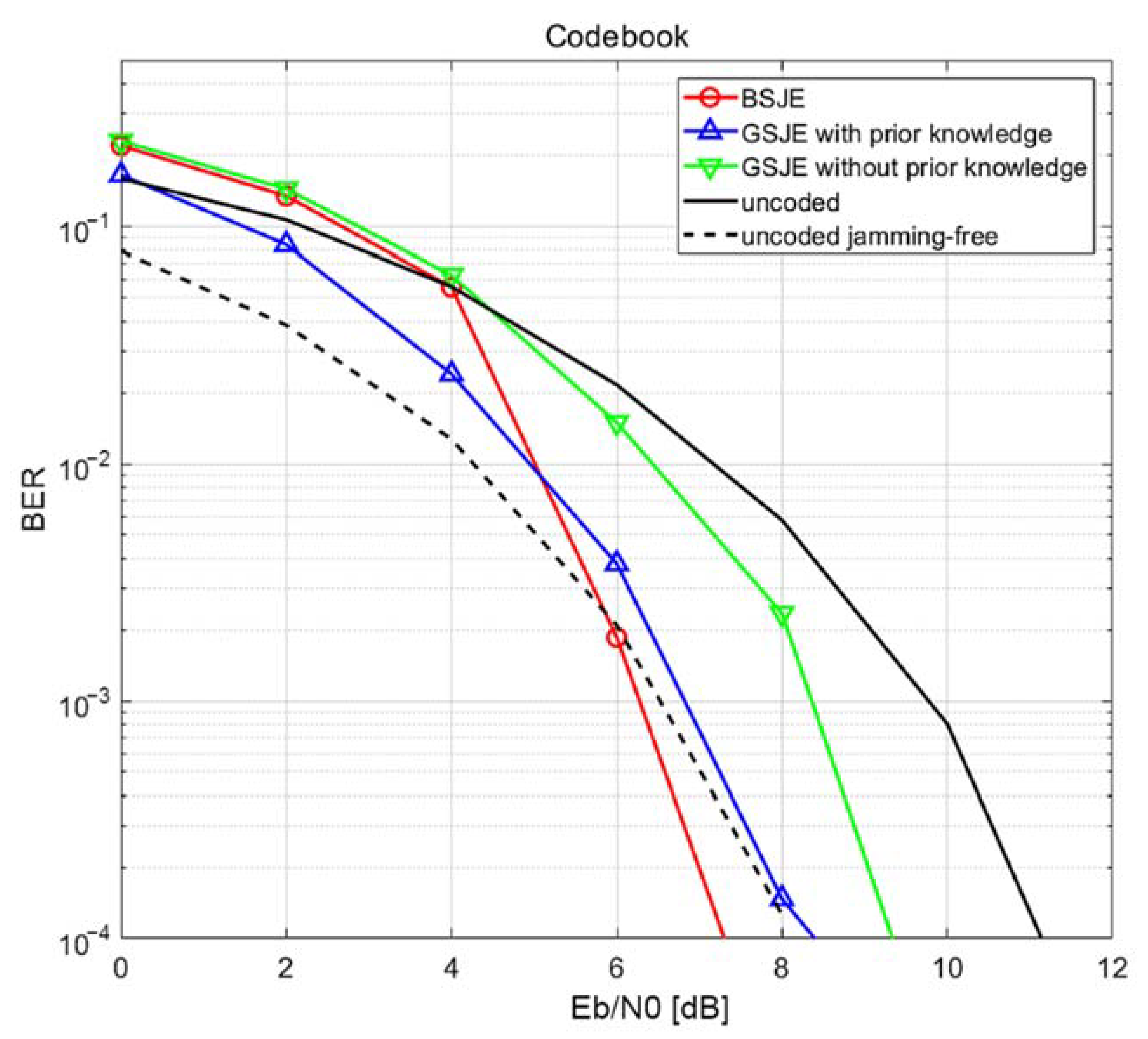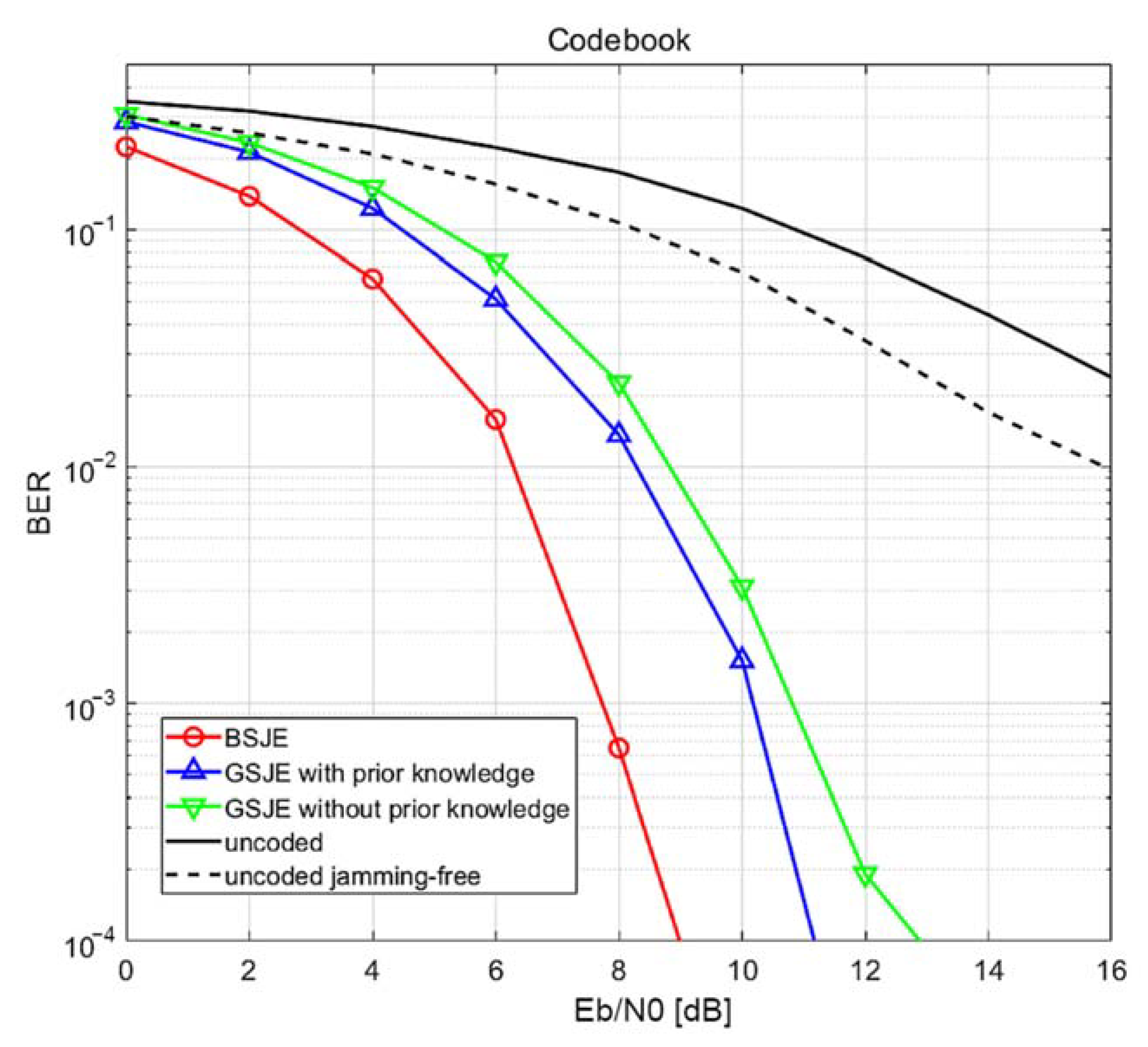As illustrated in Figure 8, the BER of the proposed method using the BSJE and GSJE algorithms with perfect prior knowledge approaches the BER of jamming-free QPSK as $E_b/N_0$ grows. In contrast, the BER of the GSJE without any prior knowledge cannot achieve anti-jamming performance. Furthermore, if the proposed codeword is drawn using the codebook method, the BER of the proposed method with the BSJE algorithm outperforms that of the jamming-free QPSK, as illustrated in Figure 9. Thus, the proposed method achieves a coding gain while simultaneously having an anti-jamming property.

Figure 9 and Figure 10 illustrate the BER performance of the proposed system over a frequency-selective fading channel. The simulation was performed over a frequency-selective fading channel with frequency-domain channel coefficients following an i.i.d. CSCG random distribution $\mathcal{C}\mathcal{N}(0,I)$, with the other parameters being identical to those in the AWGN channel simulation. Because several subbands have significantly low gain, the BER of the uncoded QPSK signal is significantly more degraded than that in the AWGN channel simulation. In contrast, the BER degradation of the proposed method is tolerable when compared to that of the uncoded QPSK. The method using BSJE demonstrates the highest performance, and the method using GSJE shows the lowest performance among the proposed methods. Consistent with the AWGN channel simulation, the performance of the codebook method illustrated in Figure 11 is superior to that of the linear Gaussian method illustrated in Figure 10.

7. Conclusions

In this paper, a novel covert anti-jamming communication system was proposed. The proposed system exploited the Gaussian-coded time-frequency modulation method to obtain covertness. As the signal samples of the proposed system followed Gaussian distributions, the signal was less detectable than the traditional binary modulated signals. We proposed the SSR-algorithm-based SJE algorithms to estimate and remove the effects of hostile jamming. In contrast to previous studies, the proposed system used the Gaussian codebook method to achieve a coding gain when the finite-field messages were encoded. We analyzed the undetectability of the proposed system as a measurement of the covertness of communications, and compared the undetectability with that of the conventional binary modulated system. We also demonstrated its BER performance through numerical simulations. The proposed system can be applied in eavesdropping- and jamming-critical applications, such as military communications in electronic warfare scenarios.

References

1. Wyner, A.D. The Wire-Tap Channel. Bell Syst. Tech. J. 1975, 54, 1355–1387. [Google Scholar] [CrossRef]
2. Bash, B.A.; Goeckel, D.; Towsley, D.; Guha, S. Hiding Information in Noise: Fundamental Limits of Covert Wireless Communication. IEEE Commun. Mag. 2015, 53, 26–31. [Google Scholar] [CrossRef] [Green Version]
3. He, B.; Yan, S.; Zhou, X.; Lau, V.K.N. On Covert Communication with Noise Uncertainty. IEEE Commun. Lett. 2017, 21, 941–944. [Google Scholar] [CrossRef] [Green Version]
4. Sklar, B. Digital Communications: Fundamentals and Applications, 2nd ed.; Prentice Hall, Inc.: Upper Saddle River, NJ, USA, 2001. [Google Scholar]
5. Marshall, T. Coding of Real-Number Sequences for Error Correction: A Digital Signal Processing Problem. IEEE J. Sel. Areas Commun. 1984, 2, 381–392. [Google Scholar] [CrossRef]
6. Wang, Z.; Giannakis, G.B. Complex-Field Coding for OFDM over Fading Wireless Channels. IEEE Trans. Inf. Theory 2003, 49, 707–720. [Google Scholar] [CrossRef]
7. Candes, E.J.; Tao, T. Decoding by Linear Programming. IEEE Trans. Inf. Theory 2005, 51, 4203–4215. [Google Scholar] [CrossRef] [Green Version]
8. Donoho, D.L. Compressed Sensing. IEEE Trans. Inf. Theory 2006, 52, 1289–1306. [Google Scholar] [CrossRef]
9. Chen, C.; Zhuo, Y. A Research on Anti-Jamming Method Based on Compressive Sensing for OFDM Analogous System. In Proceedings of the 2017 IEEE 17th International Conference on Communication Technology (ICCT), Chengdu, China, 27–30 October 2017; pp. 655–659. [Google Scholar]
10. Huan, S.; Dai, G.; Luo, G.; Ai, S. Bayesian Compress Sensing Based Countermeasure Scheme Against the Interrupted Sampling Repeater Jamming. Sensors 2019, 19, 3279. [Google Scholar] [CrossRef] [Green Version]
11. Liu, B.; Gui, G.; Matsushita, S.-Y.; Xu, L. Compressive Sensing Based Direction-of-Arrival Estimation in MIMO Radars in Presence of Strong Jamming via Blocking Matrix. In Proceedings of the 2018 IEEE 10th Sensor Array and Multichannel Signal Processing Workshop (SAM), Sheffield, UK, 8–11 July 2018; pp. 292–296. [Google Scholar]
12. Forouzesh, M.; Azmi, P.; Kuhestani, A.; Yeoh, P.L. Covert Communication and Secure Transmission over Untrusted Relaying Networks in the Presence of Multiple Wardens. IEEE Trans. Commun. 2020, 68, 3737–3749. [Google Scholar] [CrossRef]
13. Yu, J.; Yao, Y.-D. Detection Performance of Chaotic Spreading LPI Waveforms. IEEE Trans. Wirel. Commun. 2005, 4, 390–396. [Google Scholar] [CrossRef] [Green Version]
14. Sedaghatnejad, S.; Farhang, M. Detectability of Chaotic Direct-Sequence Spread-Spectrum Signals. IEEE Wirel. Commun. Lett. 2015, 4, 589–592. [Google Scholar] [CrossRef]
15. Shahzad, K.; Zhou, X.; Yan, S.; Hu, J.; Shu, F.; Li, J. Achieving Covert Wireless Communications Using a Full-Duplex Receiver. IEEE Trans. Wirel. Commun. 2018, 17, 8517–8530. [Google Scholar] [CrossRef] [Green Version]
16. Beck, A.; Teboulle, M. A Fast Iterative Shrinkage-Thresholding Algorithm for Linear Inverse Problems. SIAM J. Imaging Sci. 2009, 2, 183–202. [Google Scholar] [CrossRef] [Green Version]
17. Yang, J.; Zhang, Y. Alternating Direction Algorithms for 1-Problems in Compressive Sensing. SIAM J. Sci. Comput. 2011, 33, 250–278. [Google Scholar] [CrossRef]
18. Tropp, J.A.; Gilbert, A.C. Signal Recovery from Random Measurements Via Orthogonal Matching Pursuit. IEEE Trans. Inf. Theory 2007, 53, 4655–4666. [Google Scholar] [CrossRef] [Green Version]
19. Tropp, J.A. Greed Is Good: Algorithmic Results for Sparse Approximation. IEEE Trans. Inf. Theory 2004, 50, 2231–2242. [Google Scholar] [CrossRef] [Green Version]
20. Scott, A.L. Effects of Cyclic Prefix Jamming Versus Noise Jamming in OFDM Signals; Air Force Institute of Technology: Dayton, OH, USA, 2011. [Google Scholar]
21. Shahriar, C.; La Pan, M.; Lichtman, M.; Clancy, T.C.; McGwier, R.; Tandon, R.; Sodagari, S.; Reed, J.H. PHY-Layer Resiliency in OFDM Communications: A Tutorial. IEEE Commun. Surv. Tutor. 2015, 17, 292–314. [Google Scholar] [CrossRef]
22. Xiao, L.; Chen, T.; Liu, J.; Dai, H. Anti-Jamming Transmission Stackelberg Game with Observation Errors. IEEE Commun. Lett. 2015, 19, 949–952. [Google Scholar] [CrossRef]
23. Yang, D.; Xue, G.; Zhang, J.; Richa, A.; Fang, X. Coping with a Smart Jammer in Wireless Networks: A Stackelberg Game Approach. IEEE Trans. Wirel. Commun. 2013, 12, 4038–4047. [Google Scholar] [CrossRef]
24. Giri, R.; Rao, B. Type I and Type II Bayesian Methods for Sparse Signal Recovery Using Scale Mixtures. IEEE Trans. Signal Process. 2016, 64, 3418–3428. [Google Scholar] [CrossRef]
25. Stojnic, M.; Weiyu, X.; Hassibi, B. Compressed Sensing—Probabilistic Analysis of a Null-Space Characterization. In Proceedings of the 2008 IEEE International Conference on Acoustics, Speech and Signal Processing, Las Vegas, NV, USA, 31 March–4 April 2008; pp. 3377–3380. [Google Scholar]
26. Xu, W.; Bai, E.-W.; Cho, M. Toeplitz Matrix Based Sparse Error Correction in System Identification: Outliers and Random Noises. In Proceedings of the 2013 IEEE International Conference on Acoustics, Speech and Signal Processing, Vancouver, BC, USA, 26–31 May 2013; pp. 6640–6644. [Google Scholar]
27. Raskutti, G.; Wainwright, M.J.; Yu, B. Minimax Rates of Estimation for High-Dimensional Linear Regression Over q-Balls. IEEE Trans. Inf. Theory 2011, 57, 6976–6994. [Google Scholar] [CrossRef] [Green Version]
28. Arias-Castro, E.; Eldar, Y.C. Noise Folding in Compressed Sensing. IEEE Signal Process. Lett. 2011, 18, 478–481. [Google Scholar] [CrossRef] [Green Version]
29. Mallat, S.G.; Zhang, Z. Matching Pursuits with Time-Frequency Dictionaries. IEEE Trans. Signal Process. 1993, 41, 3397–3415. [Google Scholar] [CrossRef] [Green Version]
30. Needell, D.; Tropp, J.A. CoSaMP: Iterative Signal Recovery from Incomplete and Inaccurate Samples. Appl. Comput. Harmon. Anal. 2009, 26, 301–321. [Google Scholar] [CrossRef] [Green Version]
31. Liu, E.; Temlyakov, V.N. The Orthogonal Super Greedy Algorithm and Applications in Compressed Sensing. IEEE Trans. Inf. Theory 2012, 58, 2040–2047. [Google Scholar] [CrossRef]
32. Chrétien, S.; Hero, A.O. On EM Algorithms and Their Proximal Generalizations. ESAIM Probab. Stat. 2008, 12, 308–326. [Google Scholar] [CrossRef] [Green Version]
33. Kay, S.M. Fundamentals of Statistical Signal Processing: Estimation Theory, 1st ed.; Prentice Hall, Inc.: Hoboken, NJ, USA, 1993. [Google Scholar]
34. Tandra, R.; Sahai, A. SNR Walls for Signal Detection. IEEE J. Sel. Top. Signal Process. 2008, 2, 4–17. [Google Scholar] [CrossRef] [Green Version]
35. Han, T.S.; Verdu, S. Approximation Theory of Output Statistics. IEEE Trans. Inf. Theory 1993, 39, 752–772. [Google Scholar] [CrossRef] [Green Version]
36. Lloyd, S. Least Squares Quantization in PCM. IEEE Trans. Inf. Theory 1982, 28, 129–137. [Google Scholar] [CrossRef]
37. Moller, U.; Galicki, M.; Baresova, E.; Witte, H. An Efficient Vector Quantizer Providing Globally Optimal Solutions. IEEE Trans. Signal Process. 1998, 46, 2515–2529. [Google Scholar] [CrossRef]
38. Pages, G.; Printems, J. Optimal Quadratic Quantization for Numerics: The Gaussian Case. Monte Carlo Methods Appl. 2003, 9, 135–165. [Google Scholar] [CrossRef]
39. Snapdragon 855 Mobile Platform. Available online: https://www.qualcomm.com/products/snapdragon-855-mobile-platform (accessed on 25 February 2020).
40. USRP-2900 Specifications—National Instruments. Available online: https://www.ni.com/pdf/manuals/374924c (accessed on 20 April 2021).
41. Aref, M.A.; Jayaweera, S.K.; Machuzak, S. Multi-Agent Reinforcement Learning Based Cognitive Anti-Jamming. In Proceedings of the 2017 IEEE Wireless Communications and Networking Conference (WCNC), San Francisco, CA, USA, 19–22 March 2017; pp. 1–6. [Google Scholar]
42. Wu, Y.; Wang, B.; Liu, K.J.R.; Clancy, T.C. Anti-Jamming Games in Multi-Channel Cognitive Radio Networks. IEEE J. Sel. Areas Commun. 2012, 30, 4–15. [Google Scholar] [CrossRef] [Green Version]
43. C6000 Power-Optimized DSP|Floating Point DSP Processor|Overview|DSP|TI.Com. Available online: http://www.ti.com/processors/digital-signal-processors/c6000-floating-point-dsp/overview.html (accessed on 16 March 2020).
44. Sharma, G.; Agarwala, A.; Bhattacharya, B. A Fast Parallel Gauss Jordan Algorithm for Matrix Inversion Using CUDA. Comput. Struct. 2013, 128, 31–37. [Google Scholar] [CrossRef]
45. Yu, D.; He, S.; Huang, Y.; Yu, G.; Yang, L. A Fast Parallel Matrix Inversion Algorithm Based on Heterogeneous Multicore Architectures. In Proceedings of the 2015 IEEE Global Conference on Signal and Information Processing (GlobalSIP), Orlando, FL, USA, 14–16 December 2015; pp. 903–907. [Google Scholar]
46. Quan, Y.; Li, Y.; Gao, X.; Xing, M. FPGA Implementation of Real-Time Compressive Sensing with Partial Fourier Dictionary. Int. J. Antennas Propag. 2016, 2016, e1671687. [Google Scholar] [CrossRef] [Green Version]
47. Kim, S.; Yun, U.; Jang, J.; Seo, G.; Kang, J.; Lee, H.-N.; Lee, M. Reduced Computational Complexity Orthogonal Matching Pursuit Using a Novel Partitioned Inversion Technique for Compressive Sensing. Electronics 2018, 7, 206. [Google Scholar] [CrossRef] [Green Version]
48. Nguyen, V.Q.; Park, S.Y. High-Performance ASIC Realization of Orthogonal Matching Pursuit Algorithm. IEICE Electron. Express 2018, 15, 20180075. [Google Scholar] [CrossRef] [Green Version]
49. Cha, S.H.; Shin, M.; Ham, J.-H.; Chung, M.Y. Robust Mobility Management Scheme in Tactical Communication Networks. IEEE Access 2018, 6, 15468–15479. [Google Scholar] [CrossRef]
50. Chen, G.; Sun, P.; Zhang, J. Repair Strategy of Military Communication Network Based on Discrete Artificial Bee Colony Algorithm. IEEE Access 2020, 8, 73051–73060. [Google Scholar] [CrossRef]
51. Davenport, M.A.; Wakin, M.B. Analysis of Orthogonal Matching Pursuit Using the Restricted Isometry Property. IEEE Trans. Inf. Theory 2010, 56, 4395–4401. [Google Scholar] [CrossRef] [Green Version]
Figure 1. Tactical wireless communication system under an electronic warfare scenario.
Applsci 11 03759 g001
Figure 2. Block diagram of the proposed system. The message is encoded by Gaussian coding, described in Section 2.2. Alice transmits the codeword to Bob and Eve after a time-frequency modulation, introduced in Section 3.1. Bob estimates and removes the effect of the jammer by using the sparse jamming estimation algorithm proposed in Section 3.4, in order to decode the message from Alice. Meanwhile, Eve aims to determine if the signal is present or not. The signal detection by Eve is discussed in Section 4.
Applsci 11 03759 g002
Figure 3. Time-domain waveform of (a) proposed signal, (b) noise, and (c) signal with noise under additive white Gaussian noise (AWGN) channel with a signal-to-noise ratio (SNR) of 0 dB.
Applsci 11 03759 g003
Figure 4. Concatenation coding method. The message is first encoded using the outer code and then again using the Gaussian linear block code (LBC).
Applsci 11 03759 g004
Figure 5. Comparison between proposed signal and frequency-hopping signal in the time-frequency domain: (a) proposed signal with orthogonal frequency-division multiplexing and (b) frequency-hopping signal.
Applsci 11 03759 g005
Figure 6. Wiretap channel model.
Applsci 11 03759 g006
Figure 7. Per-symbol detection probability of proposed Gaussian and conventional binary symbols: (a) false alarm probability of 0.1 ( α = 1.645 ), (b) false alarm probability of 0.01 ( α = 2.576 ).
Applsci 11 03759 g007
Figure 8. Bit error rate (BER) performance of the proposed system in an AWGN channel at JNR = 0 dB for the linear Gaussian method.
Applsci 11 03759 g008
Figure 9. BER performance of the proposed system in an AWGN channel at JNR = 0 dB for the codebook method.
Applsci 11 03759 g009
Figure 10. BER performance of the proposed system over a frequency-selective channel at JNR = 0 dB for the linear Gaussian method.
Applsci 11 03759 g010
Figure 11. BER performance of the proposed system over a frequency-selective channel at JNR = 0 dB for the codebook method.
Applsci 11 03759 g011