Article

Design and Modelling of an Amphibious Spherical Robot Attached with Assistant Fins

Robotics Institute, School of Mechanical Engineering and Automation, Beihang University, Beijing 100191, China
*
Author to whom correspondence should be addressed.
Appl. Sci. 2021, 11(9), 3739; https://doi.org/10.3390/app11093739
Submission received: 26 March 2021 / Revised: 16 April 2021 / Accepted: 19 April 2021 / Published: 21 April 2021
(This article belongs to the Special Issue Modelling and Control of Mechatronic and Robotic Systems, Volume II)

Abstract

:
Mobile robots that can survive in unstructured wildernesses is essential in many applications such as environment detecting and security surveillance. In many of these applications, it is highly desirable that the robot can adapt robustly to both terrestrial environment and aquatic environment, and translocate swiftly between various environments. A novel concept of amphibious spherical robot with fins is proposed in this paper, capable of both terrestrial locomotion and aquatic locomotion. Unlike the traditional amphibious robots, whose motions are commonly induced by propellers, legs or snake-like tandem joints, the proposed amphibious spherical robot utilizes the rolling motion of a spherical shell as the principal locomotion mode in the aquatic environment. Moreover, spinning motion of the spherical shell is used to steer the spherical robot efficiently and agilely; several fins are attached to the outer spherical shell as an assistance to the rolling motion. These two motion modes, rolling and spinning, can be used unchangeably in the terrestrial environment, leading to a compact and highly adaptive design of the robot. The work introduced in this paper brings in an innovative solution for the design of an amphibious robot.

1. Introduction

Amphibious robots are designed to cope with drudgeries involving miscellaneous terrains, such as lakes, wetlands, shallows and pipelines [1,2]. Compared with a robot moving only on land or underwater, which is easily stuck in the junction area between the land and the water, amphibious robots are capable of both aquatic locomotion and terrestrial locomotion, which are especially suitable for applications in unknown environments, potentially with complex terrains. Tasks calling for this kind of robots include environment detecting, wild exploring, security surveillance as well as scientific inspecting [3].
A variety of amphibious robots have been developed by researchers in recent years. As one of the typical amphibious robots, snake-like robots are inspired by the locomotion mode of a snake as well as a lamprey. A snake-like robot called HELIX is developed by Takayama and Hirose to verify the propulsion principle that helical motion can be created by successive distortions of articulated body segments [4]. The design of one unit of HELIX, including a special spherical mechanism and two servo motors, is introduced in detail by the same authors. As a modified prototype of HELIX, ACM-R5 bears impressive performance in terms of its dexterous locomotion capacity. Underwater swimming fins are attached around the outer surface of each unit to assist the underwater motion, with passive wheels attached on the tip of each fin in order to improve the on-land locomotion performance [2,5]. The AmphiBot robots, a series of amphibious snake-like robots capable of swimming in water and crawling on land, are designed by Ijspeert and Crespi et al. [6]. A central pattern generator (CPG)-based controller is used to generate lateral undulation for this kind of robot [7,8]. Some key parameters that produce fast locomotion gaits, such as the amplitude of oscillation, frequency and wavelength, are identified by a series of experiments. An improved version of AmphiBot, named Salamandra robotica, equipped with a passive tail and four active 3-DOF limbs, is also introduced [9]. To make the snake-like robot to follow a desired path, a straight line path following controller is proposed by Kelasidi et al. [10,11].
Another type of amphibious robots is equipped with flippers that act as paddles in water and as legs on land. Using six paddles for propulsion, AQUA is suitable for navigating in shallow-water environment [12,13]. With the help of an acoustic-based localization system and a vision-based localization system, AQUA obtained the ability to revisit a previously visited site autonomously [14,15]. To enhance its climbing ability, Whegs IV combines two similar body segments with wheel-leg propellers [16,17]. AmphiHex-I obtains versatile gaits with the aid of transformable flipper legs, which makes it flexible in transforming propulsion mechanisms [18]. Its improved version with variable stiffness legs and CPG-based control strategy is also introduced [19]. A quadrupedal micro-robot weighs only several grams is introduced by Cheng et al. [20], which uses passive flaps to swim forward and adjust direction.
Some robots with spherical shape have also drawn researchers’ attention. The Groundbot, an amphibious spherical robot that accomplishes its propulsion system by displacing the center of mass, is introduced by Kaznov et al. [21]. Groundbot shows good robustness in the waypoint following mode. An amphibious spherical robot which combines two actuating systems, including the quadruped walking system for terrestrial locomotion and the water-jet propulsion system for underwater locomotion, is designed by Guo et al. [22,23]. A micro-robot which is used as a manipulator and a monitor can be carried and deployed by this amphibious spherical robot. An amphibious spherical robot uses pendulum to move on land and propeller to move in the water is developed by Li et al. [24]. A spherical rotary paddle called Omni-Paddle is proposed to form a robot that mainly moves on the boarder of water and ground [25]. Four Omni-Paddles are disposed in a radical pattern around the outside of the robot, with which the robot is capable of moving towards any direction. The Omni-Paddle works as not only a driving mechanism but also a source of buoyancy in one prototype of the robot.
Each of the amphibious robots mentioned above has its advantages and disadvantages. A snake-like robot adapts well to complex terrains; however, it usually needs many units of bodies in order to achieve a high terrain adaptability, as a result requiring a large amount of motors. This leads to low robustness and high energy consumption, which is the bottleneck in field applications. A robot equipped with water-jet propulsion system can control its position and attitude precisely underwater. However, another actuation system is needed for its locomotion on land, resulting in a complex actuation system and extra weight. A robot with paddles mimics the locomotion modes used by amphibians such as ducks and turtles, which is advantageous in that it uses the same set of actuation system for both on land and in water locomotion; however, it calls for complex algorithms for gait planning in order to reach dynamic stability. In addition, the existence of feet increases risk of being entwined by water plants or shrubs.
A spherical robot bears very few motors that are sufficient for both on land and in water locomotion. Because of its inherent sealing characteristic, good stability and low energy cost, spherical robots have a great potential to be used in amphibious locomotion in field applications. However, the relatively slow locomotion speed on the water due to frictionless spherical shell and the poor maneuverability are main hindrances in using a spherical robot as an amphibian. To overcome these limitations, a novel amphibious spherical robot design is proposed in this paper, by attaching assistant fins to the outside surface of the spherical shell to increase its locomotion speed, and by using a combination of pendulum and rotator as the Inside Drive Unit (IDU) to propel the robot agilely. It is shown that this design strategy significantly improves the mobility capacity of the robot, and enhances its resistance to environment undulation, making it practicable to use a spherical robot both on land and on water.
The remainder of the paper is organized as follows. In Section 2, the mechanical design, the electrical actuation and the control system of the amphibious spherical robot are introduced. In Section 3, the equations of the robot’s motion are deduced based on kinematic analyses and force analyses. In Section 4, simulations of the dynamic model are presented, and the experiments to test the performance of the robot are described in detail. Finally, the conclusion is given in Section 5.

2. Mechanical Structure and Electrical Actuation and Control System

2.1. Design Objectives

The design objectives of the amphibious spherical robot project are:
  • the ability to navigate on the water and on the land with exactly the same driving mechanism;
  • a sealed structure, enclosing its vulnerable components to protect them from outside environments, e.g., water, sand and gas, so as to make it capable of surviving harsh environments;
  • this robot can be remotely handled by an operator.
These aims are achieved by the proposed amphibious spherical robot scheme, which consists of a spherical robot and a radio frequency (RF) remote controller.

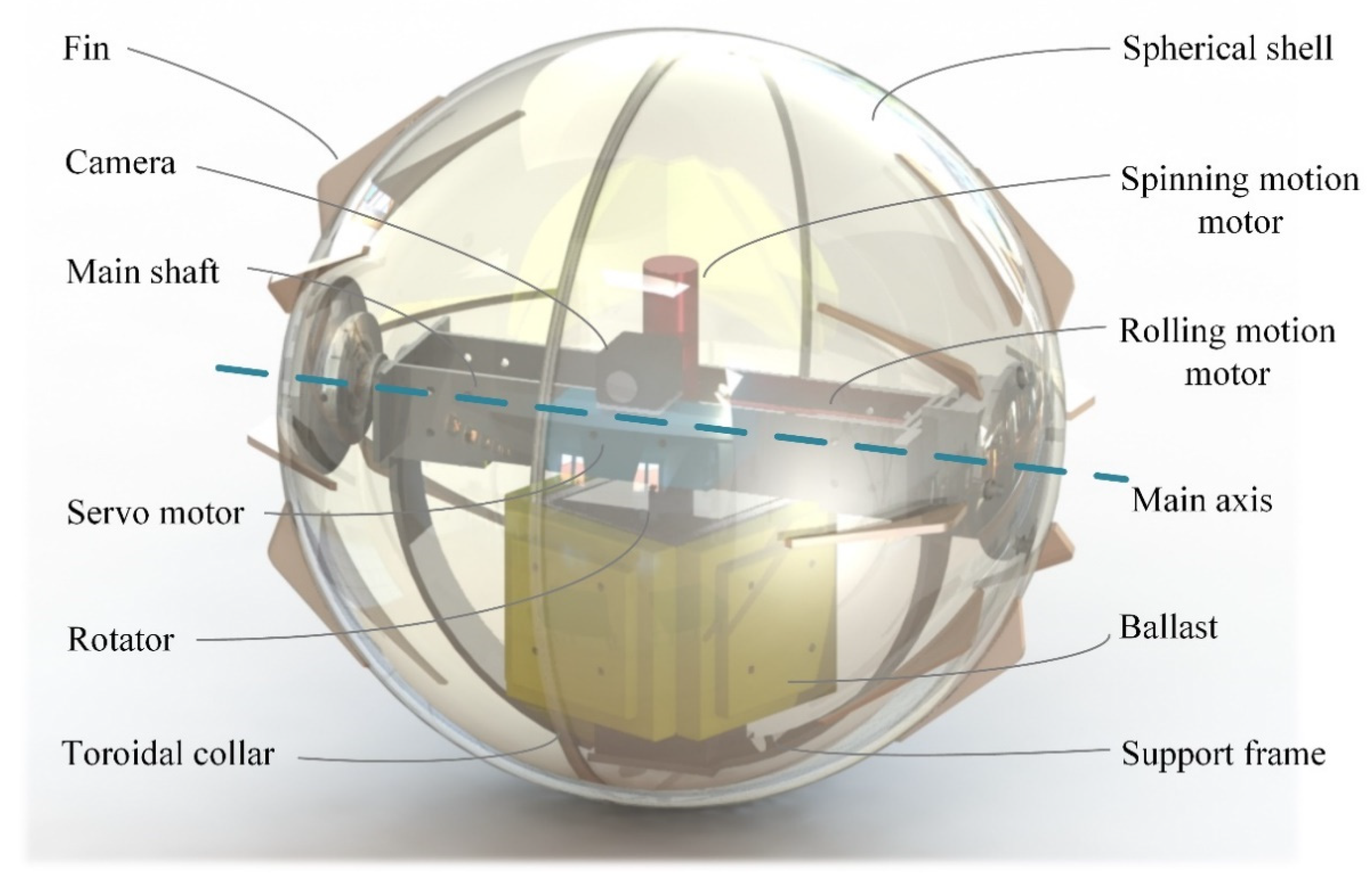
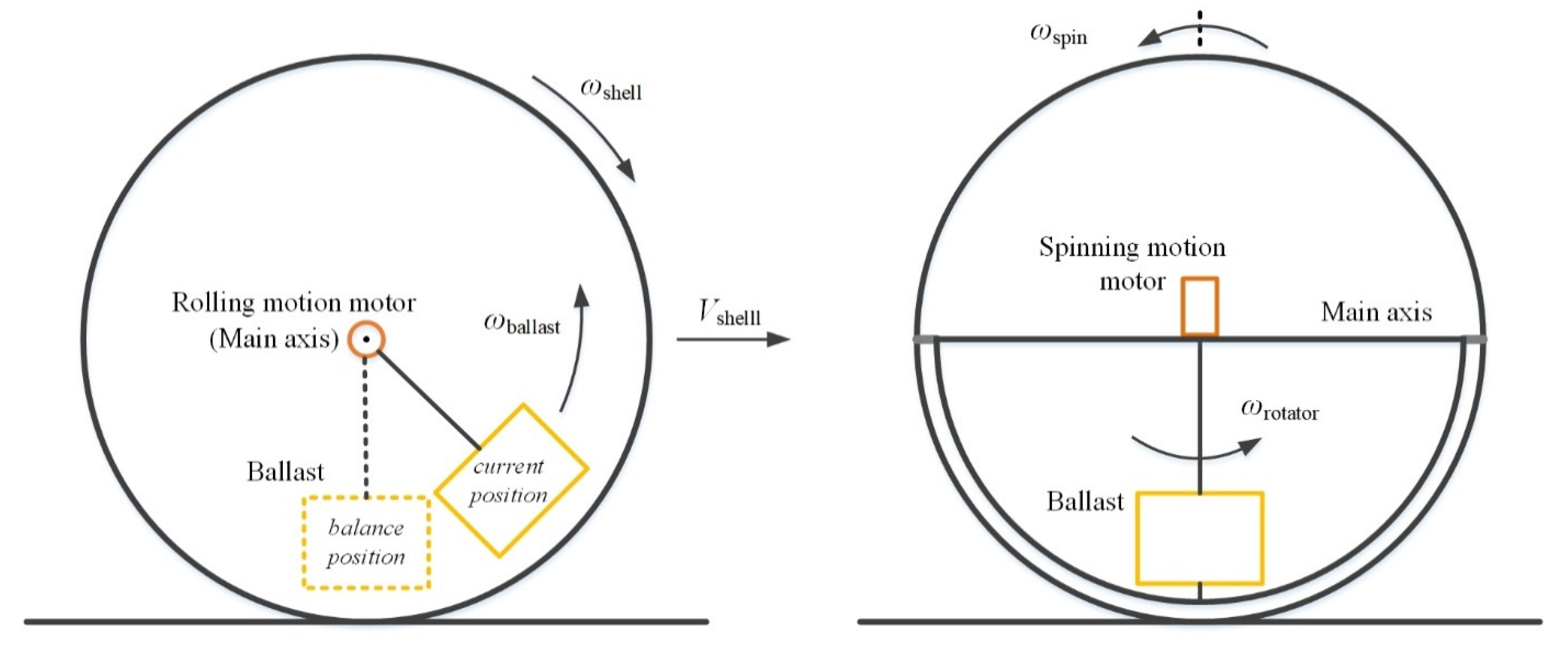
2.2. Introduction of the Developed Spherical Robot

The spherical robot introduced here is a modified type aiming at amphibious applications, which is originated from traditional spherical robots [26,27]. The spherical robot is mainly composed of two parts: a hollow spherical shell and an IDU, as shown in Figure 1. The spherical shell acts as both a wheel and a shelter; while the IDU, consisting of components inside the spherical shell, acts as the driving unit of the whole robot.
The hollow spherical shell consists of two hemispheric shells made of acrylic material, which makes it transparent and with little radio interference. A toroidal collar is attached to the great circle of one hemispherical shell, acting as an installation reference for the other hemispherical shell. Some subtriangular fins are adhered onto the outside surface of the spherical shell, in order to improve the robot’s locomotion performance when navigating on the water.
The IDU is mounted completely in the inner space of the hollow spherical shell. Its mechanical structure mainly contains a main shaft, a support frame and a rotator. Two basic motion modes of the spherical robot, i.e., rolling motion and spinning motion, can be actuated by the IDU.
The main shaft lies along the sphere’s main axis which is fixed relative to the spherical shell during motion, making it parallel to the ground in a stationary state. Two DC motors are mounted on the main shaft to actuate the IDU, named rolling motion motor and spinning motion motor, respectively. The rolling motion motor is placed along the main axis. When this motor starts to rotate, the IDU will depart from its balanced position and begin to rotate about the main axis. The torque exerted onto the spherical shell will accumulate as a consequence. The spherical shell starts to roll as soon as this torque exceeds the friction resistance, resulting in the linear motion of the whole spherical robot. The spinning motion motor is placed perpendicular to the sphere’s main axis, and is along the diameter that passes through the contact point in a stationary state. A rotator is connected to this motor through a coupler. When the angular velocity of the rotator is changed by activating the spinning motion motor, the angular momentum of the rotator succeeds to change. As a result of the conservation of angular momentum principle, the spherical shell will spin in the direction that opposite to the change of angular momentum.
The principle of those two motion modes is illustrated in Figure 2.
A curved trajectory can be achieved upon combining the rolling motion mode and spinning motion mode, i.e., upon steering the robot when it is moving forward or backward.
The rotator is placed in the interspace between the main shaft and the semi-circular support frame, which is fixed beneath the main shaft. The rotator is composed of a few pieces of ballasts, which are made by stainless steel in order to supply enormous mass and moment of inertial. In order to test the relationship between the depth of immersion and locomotion performance of the spherical robot, the number of ballasts is designed to be adjustable by splitting the ballasts into pieces with different mass. So, the total mass of the rotator can be simply changed by adding or removing some pieces of the ballasts.
Sixteen subtriangular fins, eight on each side, are fixed on the outside surface of the spherical shell to improve the locomotion performance on the water. By applying prudent control strategies, these fins will not have any collision with the ground when the robot is moving on land. By contrast, they will immerge into the water when the robot is navigating on the water. Two factors—the first is the number of fins attached to the spherical shell, and the second is the shape of the fin—are believed to have significant impact on the locomotion performance of the robot on the water.
Apart from those driving facilities mentioned above, the waterproof ability is of great importance for the amphibious spherical robot. Several approaches have been proposed to keep loads inside the spherical shell from water.

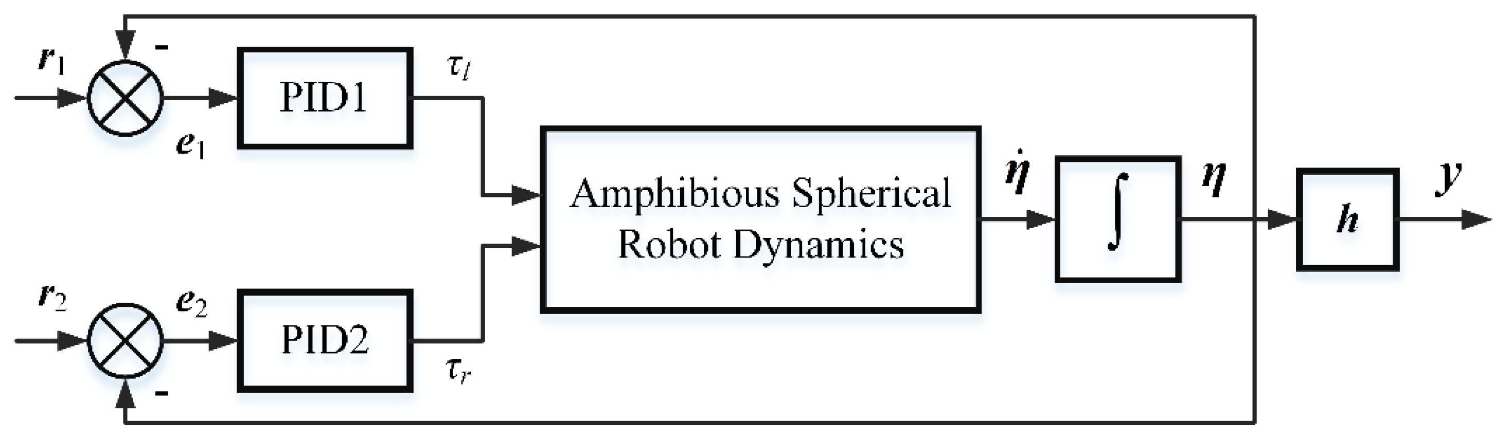
2.3. Electrical Actuation and Control System of the Robot

The electrical actuation and control system consist of two DC motors, a servo motor, two electronic speed controls (ESC) working as motor drive units, a signal receiver, a camera and power supply module. It provides the power and impetus needed for the spherical robot. It receives the control signal transmitted by the RF remote controller and the signal emitter, then outputs impetus to the mechanical structure of the IDU and the spherical shell. Its schematic is shown in Figure 3.
The signal receiver is used to collect radio frequency signals emitted from the RF remote controller. After some valid signals arrived, it will decode the received signals and then generate control signals for corresponding motors. The signal receiver connects to two DC motors through two ESCs respectively and one servo motor directly. These three motors occupied three of the nine output channels of the signal receiver. The power of the signal receiver is supplied by a battery eliminator circuit (BEC) incorporated in one of the ESCs. The ESC, mainly used for brushed DC motors, acts as motor driver in this application. It converts the digital signals from the signal receiver to voltages exerted upon the motors. Those ESCs are powered by the power supply module. The output voltage of the ESC will change with the variation of the input signal received from the signal receiver. As a result, rotation speed of these DC motors will change at the same time.
To record videos of the robot’s surroundings, a digital camera is mounted inside the spherical shell. The servo motor mounted on the main shaft is used for adjusting the vision field of the camera in horizontal plane. This servo motor is connected directly to the signal receiver because it consumes power within the safety threshold of the signal receiver. As a micro wireless signal transmitter is integrated into the camera, videos produced by the camera can be transmitted to the RF remote controller in time.
A 24 V lithium battery is used as the power supply module for the robot, and a wireless switch is placed between the power supply module and those power consuming devices. The on-off state of the power supply is then achieved by sending corresponding signals to the wireless switch from an external signal emitter.
The control block diagram of the robot system is shown in Figure 4. Two PID controllers are implemented in order to control the two system inputs, i.e., τ l and τ r , generated by the rolling motion motor and the spinning motion motor, respectively.
The PID1 controller is used in the basic rolling motion mode, while the PID2 controller is used in the basic spinning motion mode, when the robot needs to adjust its direction. These two controllers work in cooperation when the robot is operating in a curved trajectory.

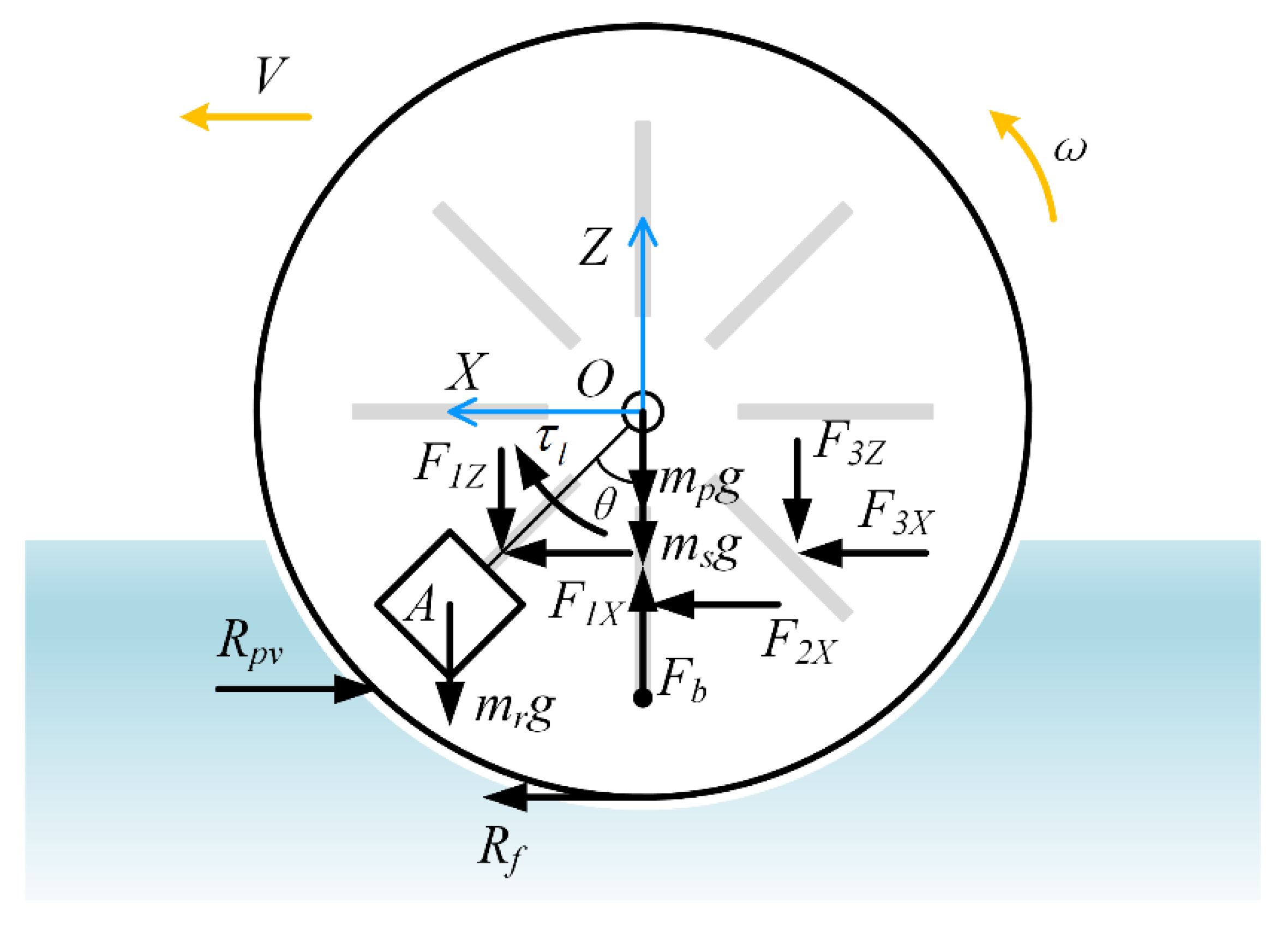
3. Dynamic Model of the Robot

The amphibious spherical robot is modelled as a system consists of three rigid bodies, the spherical shell with its attached assistant fins, the IDU platform and the rotator. Assumptions about these three components are (1) the spherical shell is a uniform hollow spherical shell whose radius is R; the total mass of the spherical shell and its attached assistant fins is m s while each fin has mass m f ; (2) the IDU platform is considered as a uniform rectangular bar with mass m p , length 2R, neglecting its structural details; it is mounted along the main axis with its center of mass locating at the center of spherical shell; (3) the rotator is a hollow cube with its mass m r distributed on the four side faces of the cube; the distance between the center of mass of the rotator A and the main axis is l O A .

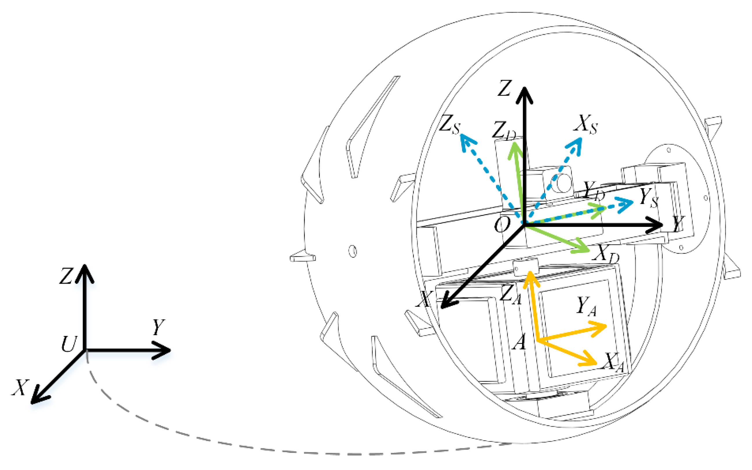
3.1. Coordinate Frames

Coordinate frames attached to those three rigid bodies are shown in Figure 5. An inertial frame U-XYZ is set with its X axis pointing to the east of the locus, its Y axis pointing to the north and its Z axis pointing vertically upward. The frame O-XYZ is parallel to the inertial frame, with its origin located at the center of spherical shell O. Let OS-XSYSZS be the coordinate frame anchored to the spherical shell, whose origin is located at the point O and YS axis is always parallel to the main axis. This OS-XSYSZS frame is used to describe the configuration of the spherical shell. Let OD-XDYDZD be the body frame of the IDU platform, with its origin located also at point O, its YD axis coinciding with the YS axis and its ZD axis parallel to the rotator’s spinning axis. In addition, the A-XAYAZA frame, located at the center of mass of the rotator, is used to describe the configuration of the rotator; its ZA axis lies along the rotator’s spinning axis.
In general, eight variables η = x , y , z , ϕ , θ , ψ , α s , α r are needed to describe the states of the whole robot, among which, three variables (x, y, z) represent the center of the spherical shell, three Euler angles ϕ , θ , ψ represent the orientation of the IDU platform, the angle α s represents the angle between the body frame of the spherical shell OS-XSYSZS and the body frame of the IDU platform OD-XDYDZD; lastly, the angle α r is the spinning angle of the rotator. As these eight variables are independent of each other, they are chosen as the generalized coordinates of the robot system.

3.2. Kinematics

Kinematic parameters that are necessary for deducing the dynamic equations, i.e., the translational velocities of the center of mass of each rigid body and the angular velocities with respect to each center of mass, are presented in the following. Let r O = x , y , z be the position vector of the geometric center of the spherical shell O whose velocity is r ˙ O = x ˙ , y ˙ , z ˙ , r P = x P , y P , z P be the position vector of the center of mass of the IDU platform whose velocity equals to r ˙ O , i.e., r ˙ P = r ˙ O , and r A = x A , y A , z A be the position vector of the center of mass of the rotator A. Let   D r O A = 0 , 0 , l O A denote the position vector of the point A with respect to the OD-XDYDZD frame; r A then is
r A = r O +   D U R D r O A ,
where   D U R S O 3 denotes the rotation matrix between the U-XYZ frame and the OD-XDYDZD frame, which can be expressed in terms of the Euler angles, that is,
  D U R = c ψ c θ s ψ c ϕ + c ψ s θ s ϕ s ψ s ϕ + c ψ c ϕ s θ s ψ c θ c ψ c ϕ + s ψ s θ s ϕ c ψ s ϕ + s θ s ψ c ϕ s θ c θ s ϕ c θ c ϕ ,
where c ϕ is the shorthand for cos ϕ , s ϕ for sin ϕ , and so on. Substituting   D U R into Equation (1), we get
r A = x s ψ s ϕ + c ψ c ϕ s θ l O A , y c ψ s ϕ + s θ s ψ c ϕ l O A , z c θ c ϕ l O A .
The velocity of the rotator’s center of mass r ˙ A can be obtained by differentiating r A , its three components are
x ˙ A = x ˙ c ϕ s ψ ϕ ˙ ψ ˙ s θ + s ϕ c ψ ψ ˙ ϕ ˙ s θ + θ ˙ c ϕ c ψ c θ l O A y ˙ A = y ˙ s ϕ s ψ ψ ˙ ϕ ˙ s θ c ϕ c ψ ϕ ˙ ψ ˙ s θ + θ ˙ c ϕ s ψ c θ l O A z ˙ A = z ˙ + θ ˙ c ϕ s θ + ϕ ˙ s ϕ c θ l O A
As the rotation matrix   D U R is an orthonormal matrix,   D U R 1 =   D U R T , so
  D U R   D U R T = I 3 × 3 .
Differentiating both sides of Equation (5), we have
  D U R ˙   D U R T +   D U R ˙   D U R T T = 0 .
If we define S p : =   D U R ˙   D U R T , then S p + S p T = 0 . So S p s o 3 is an anti-symmetric matrix whose diagonal elements are all zero:
S p = 0 ψ ˙ + ϕ ˙ s θ θ ˙ c ψ + ϕ ˙ s ψ c θ ψ ˙ ϕ ˙ s θ 0 ϕ ˙ c ψ c θ + θ ˙ s ψ θ ˙ c ψ ϕ ˙ s ψ c θ ϕ ˙ c ψ c θ θ ˙ s ψ 0 .
The matrix S p can be made up from ω p = ω p x , ω p y , ω p z , the angular velocity of the IDU platform with respect to the U-XYZ frame, that is,
S p = ω ^ p = 0 ω p z ω p y ω p z 0 ω p x ω p y ω p x 0 .
The angular velocity ω p then can be deduced from S p reversely:
ω p = ϕ ˙ c ψ c θ θ ˙ s ψ , θ ˙ c ψ + ϕ ˙ s ψ c θ , ψ ˙ ϕ ˙ s θ .
Note that ω p is not a generalized velocity but a quasi-velocity. The angular velocity of the IDU platform with respect to the OD-XDYDZD frame can be obtained by coordinate transformation
  D ω p =   D U R T ω p = ϕ ˙ ψ ˙ s θ , θ ˙ c ϕ + ψ ˙ s ϕ c θ , θ ˙ s ϕ + ψ ˙ c ϕ c θ .
To deduce the angular velocity of the spherical shell, let S s : =   S U R ˙   S U R T , where   S U R is the rotation matrix between the U-XYZ frame and the OS-XSYSZS frame.   S U R can be obtained by matrix multiplication,   S U R =   D U R   S D R , where   S D R is the rotation matrix between the OD-XDYDZD frame and the OS-XSYSZS frame.   S D R can be expressed as
  S D R = c α s 0 s α s 0 1 0 s α s 0 c α s .
Substituting   S D R into the equation of   S U R ,   S U R then is
  S U R = c ψ c θ c α s s ψ s ϕ + c ψ c ϕ s θ s α s c ψ s θ s ϕ s ψ c ϕ c ψ c θ s α s + s ψ s ϕ + c ψ c ϕ s θ c α s s ψ c θ c α s + c ψ s ϕ s θ s ψ c ϕ s α s c ψ c ϕ + s ψ s θ s ϕ s ψ c θ s α s + s θ s ψ c ϕ c ψ s ϕ c α s s θ c α s c θ c ϕ s α s c θ s ϕ c θ c ϕ c α s s θ s α s .
The angular velocity of the spherical shell with respect to the U-XYZ frame, ω s = ω s x , ω s y , ω s z , can be deduced from the matrix S s , whose three components are
ω s x = ϕ ˙ c ψ c θ θ ˙ s ψ + α ˙ s c ψ s θ s ϕ c ϕ s ψ ω s y = θ ˙ c ψ + ϕ ˙ s ψ c θ + α ˙ s s ψ s θ s ϕ + c ϕ c ψ ω s z = ψ ˙ ϕ ˙ s θ + α ˙ s c θ s ϕ
Its expression with respect to the OS-XSYSZS frame are
  S ω s x = θ ˙ s ϕ s α s + ϕ ˙ c α s ψ ˙ s θ c α s + c θ c ϕ s α s   S ω s x = θ ˙ c ϕ + ψ ˙ c θ s ϕ + α ˙ s   S ω s z = ϕ ˙ s α s θ ˙ s ϕ c α s + ψ ˙ c θ c ϕ c α s s θ s α s
Then, let S a : =   A U R ˙   A U R T , where   A U R is the rotation matrix between the U-XYZ frame and the A-XAYAZA frame and   A U R =   D U R   A U R .   D U R is the rotation matrix between the OD-XDYDZD frame and the A-XAYAZA frame, which is
  A D R = c α r s α r 0 s α r c α r 0 0 0 1 .
Substituting   A D R into the equation of   A U R , we get
  A U R = c ψ c θ c α s s ψ s ϕ + c ψ c ϕ s θ s α s c ψ s θ s ϕ s ψ c ϕ c ψ c θ s α s + s ψ s ϕ + c ψ c ϕ s θ c α s s ψ c θ c α s + c ψ s ϕ s θ s ψ c ϕ s α s c ψ c ϕ + s ψ s θ s ϕ s ψ c θ s α s + s θ s ψ c ϕ c ψ s ϕ c α s s θ c α s c θ c ϕ s α s c θ s ϕ c θ c ϕ c α s s θ s α s .
The angular velocity of the rotator with respect to the U-XYZ frame, ω r = ω r x , ω r y , ω r z , can be deduced from the matrix S a , its three components are
ω r x = ϕ ˙ c ψ c θ θ ˙ s ψ + α ˙ r c ψ s θ c ϕ + s ϕ s ψ ω r y = θ ˙ c ψ + ϕ ˙ s ψ c θ + α ˙ r s ψ s θ c ϕ s ϕ c ψ ω r z = ψ ˙ ϕ ˙ s θ + α ˙ r c θ c ϕ
Its expression with respect to the A-XAYAZA frame are
  A ω r x = θ ˙ c ϕ s α r + ϕ ˙ c α r + ψ ˙ c θ s ϕ s α r s θ c α r   A ω r y = θ ˙ c ϕ c α r ϕ ˙ s α r + ψ ˙ c θ s ϕ c α r + s θ s α r   A ω r z = ψ ˙ c θ c ϕ θ ˙ s ϕ + α ˙ r
The above kinematic analyses determine parameters that are important in dynamic modeling, i.e., the velocity r ˙ O , r ˙ A as well as the angular velocity   D ω p ,   S ω s and   A ω r .

3.3. Generalized Forces

The equations of motion of the amphibious spherical robot are derived based on force analyses when the robot is navigating on the water, as shown in Figure 6. The coordinate frame O-XYZ is set with its origin located at the center of the spherical shell O and its Y axis pointing outward the paper.
Forces exerted on the spherical shell are mainly due to interactions between the fluid and the spherical shell. It includes the gravity of the spherical shell m s g , the buoyancy F b , the hydrodynamic force F h y d , the resultant force exerted on all fins F t f as well as their corresponding torques. F h y d consists of two main components, i.e., the frictional resistance R f and the pressure resistance R p v . The forces exerted on the IDU platform and the rotator are simply their gravities, m p g and m r g , respectively. Two input torques τ l and τ r are generated from the rolling motion motor and the spinning motion motor.
The buoyancy F b , the frictional resistance R f , the pressure resistance R p v and the resultant force exerted on all fins F t f are described in detail in the following.
(a)
Buoyancy
The buoyancy exerted on the spherical shell equals the gravity of the water which has the same volume as the immerged part of the spherical shell. If we set the generalized coordinate z = 0 and let H 0 represents the height from the bottom of the spherical shell to the surface of water when the robot is in static equilibrium on the water, then the buoyancy is
F b = ρ w g π R H 0 z 2 H 0 z 3 / 3 ,
where ρ w is the density of water, g is the gravitational acceleration. The center of buoyancy lies vertically below the center of sphere, its z coordinate is
z b = z 3 H 0 z 2 R 2 4 H 0 z 3 R .
(b)
Frictional Resistance
In contrast to the pure rolling motion on the ground, the amphibious spherical robot slides relative to the fluid surface when rolling on the water, as a consequence of poor frictional condition at the contact region. The frictional resistance between the spherical shell and the fluid can be derived from the theory adapted to a ship [28], assuming that it is equal to the frictional resistance on a flat plate that is equivalent to the immerged spherical shell. It should be noted that the direction of the frictional resistance on the spherical shell is the same as the robot’s moving direction, instead of being in the opposite direction in the case of a ship. As a result, the frictional resistance acts as propulsion for the amphibious spherical robot.
The frictional resistance exerted on the spherical shell R f can be written as
R f = C f + Δ C f · 1 2 ρ w V e q u 2 S w ,
where C f is the frictional resistance coefficient of an equivalent flat plate corresponding to the spherical shell; Δ C f is the roughness coefficient, determined by the roughness of the spherical shell in contact with the water; V e q u is the equivalent velocity of the robot relative to the water. S w is the wetted surface area, which can be written as
S w = 0 H 0 2 π R 2 h R 2 · 1 + h R 2 R 2 h R 2 d h = 2 π R H 0 .
The frictional resistance coefficient is determined by the Reynolds number Re, namely,
Re = V e q u · L w l ν ,
where ν is the kinematic viscosity of water; L w l represents the waterline length of the spherical shell,
L w l = 2 × 2 R H 0 H 0 2 .
An estimated value of Re for the amphibious spherical robot described in this paper is about 1.45 × 10 5 given that V e q u = 0.5   m / s , L w l = 0.33   m , the kinematic viscosity ν = 1.139 × 10 6   m 2 / s , and the temperature of the water is 15 °C. This Re value is less than the critical Reynolds number of a flat plate, which is approximately 1.0 × 10 6 . Therefore, the water flow relative to the spherical shell can be presumed as laminar flow, which is characterized by smooth, constant fluid motion. The frictional resistance coefficient C f is then given as [29]
C f = 1.328 Re 1 2 .
As the outside surface of the spherical shell is smooth, the roughness of the spherical shell barely contributes to the total resistance, so the roughness coefficient Δ C f is set as zero in the calculation.
Solving Equations (21)–(25), we have
R f = 1.328 π ν V e q u 3 L w l ρ w R H 0 .
Using Equation (26), we can obtain a roughly estimate of the frictional resistance of the spherical shell in terms of its specifications. To get an accurate value of the frictional resistance, experiment or Computational fluid dynamics (CFD) methods are necessary, which, however, are not the emphasis here.
(c)
Pressure Resistance
The hydrodynamic force exerted on the spherical shell consists of the frictional resistance and the pressure resistance. The pressure resistance is due to the decrease of pressure between the front of the spherical shell and its rear. It is difficult to separate the frictional resistance and pressure resistance theoretically. However, researchers have carried out CFD simulations and experiments to measure the resultant of those two resistances [30,31]. So, it will be possible to evaluate the pressure resistance approximately by subtracting the frictional resistance from the resultant resistance in a somewhat simple way.
The hydrodynamic force exerted on the spherical shell then can be presented in the O-XYZ frame as   O F h y d = F h X , F h Y , F h Z , its corresponding torque relative to the center of sphere is   O τ h y d = τ h X , τ h Y , τ h Z .
(d)
Resultant Force Exerted on the Fins
According to Healey et al. [32], when a fin moves relative to the water, a drag force and a lift force are exerted on the fin. The drag force D is in line with the inlet water, whose velocity is   f V w , and the lift force L is perpendicular to the inlet water. They can be calculated as follows [32]
L = 1 2 ρ w   f V w 2 S f C L max sin 2 α e ,
D = 1 2 ρ w   f V w 2 S f C D max 1 cos 2 α e ,
where S f is the cross-section area of the fin submerged in the water; the angle of attack α e is defined as the angle between the inflow water’s velocity and the cross-section plane of the fin. The maximum lift coefficient C L max is determined by the shape of the fin. C D max is the maximum drag coefficient. Both these two coefficients can be acquired by experiments.
The components of the drag force and the lift force projected in the horizontal direction and vertical direction can be calculated as:
F i X = L sin φ + α e + D cos φ + α e ,
F i Z = L cos φ + α e + D sin φ + α e ,
where F i X denotes the components of the ith fin in the X direction, F i Z denotes the components of the ith fin in the Z direction, φ is the phase angle of the fin in its rotation cycle.
The resultant force exerted on all those fins submerged in the water is the sum of forces exerted on each fin, and it can be presented in the O-XYZ frame as   O F t f = F f X , F f Y , F f Z ; its corresponding torque relative to the center of sphere is   O τ t f = τ f X , τ f Y , τ f Z .
After determining all the applied forces upon the spherical robot, it is necessary to calculate the generalized force due to nonconservative forces before we obtain the equations of motion. This will be accomplished by the principle of virtual work. The virtual work δ W j corresponding to one generalized coordinate can be calculate by multiplying the applied forces with the virtual displacement. The generalized forces can be obtained by dividing the virtual work by its corresponding generalized coordinate, that is,
Q j = δ W j / δ η j .

3.4. Equations of Motion

The equations of the spherical robot’s motion when it navigates on the surface of water are deduced by Lagrange’s methods. When evaluating the forces exerted on the robot’s components, forces that can be obtained from a potential function are conservative, and should be formulated into the potential energy. Forces associated with energy dissipation are nonconservative and should be formulated into the generalized forces. First, we need to construct the Lagrangian by calculating the kinetic energy and the potential energy of those three components of the robot.
The kinetic energy of the spherical shell is the sum of the energy due to the translational motion of its center of mass and the energy due to rotation about the center of mass, that is,
T s = 1 2 m s x ˙ 2 + y ˙ 2 + z ˙ 2 + 1 2 I s X X   S ω s x 2 + I s Y Y   S ω s y 2 + I s Z Z   S ω s z 2 ,
where I s X X , I s Y Y and I s Z Z are moments of inertia of the spherical shell about its three axes of body frame OS-XSYSZS, respectively. As the spherical shell is symmetrical, those three axes are its principle axes. The total number of fins attached to the spherical shell is 2n with n fins on each hemisphere. Each of those attached fins can be reckoned as with mass m f and radius of gyration R/2 approximately, so I s X X , I s Y Y and I s Z Z can be written as
I s X X = 2 3 m s R 2 5 6 n m f R 2 ,   I s Y Y = 2 3 m s R 2 5 6 n m f R 2 ,   I s Z Z = 2 3 m s R 2 5 6 n m f R 2 .
The gravity and the buoyancy on the spherical shell are related only to the generalized coordinates so that they are conservative, then the potential energy of the spherical shell is
V s = m s g z + ρ w g π R H 0 z 3 / 3 + H 0 z 4 / 12 .
The first term in the right-hand side of the above equation is potential energy corresponding to the gravity, and the second term is the potential energy arising from the buoyancy.
Similarly, the kinetic energy of the IDU platform is
T p = 1 2 m p x ˙ P 2 + y ˙ P 2 + z ˙ P 2 + 1 2 I p X X   D ω p x 2 + I p Y Y   D ω p y 2 + I p Z Z   D ω p z 2 ,
where I p X X , I p Y Y and I p Z Z are moments of inertia of the IDU platform about its three axes of body frame OD-XDYDZD, respectively. They can be obtained by referring to the cuboid model
I p X X = 1 12 m p 4 R 2 + l p 2 ,   I p Y Y = 1 6 m p l p 2 ,   I p Z Z = 1 12 m p 4 R 2 + l p 2 .
The potential energy of the IDU platform is
V p = m p g z P .
The kinetic energy of the rotator is
T r = 1 2 m r x ˙ A 2 + y ˙ A 2 + z ˙ A 2 + 1 2 I r X X   A ω r x 2 + I r Y Y   A ω r y 2 + I r Z Z   A ω r z 2 ,
where I r X X , I r Y Y and I r Z Z are moments of inertia of the rotator about its three axes of body frame A-XAYAZA, respectively. As the mass of the rotator is assumed to be distributed on the four side faces of the cube, each of which is a square with length l r , so these moments of inertia are
I r X X = 1 4 m r l r 2 ,   I r Y Y = 1 4 m r l r 2 ,   I r Z Z = 1 3 m r l r 2 .
The potential energy of the rotator is
V r = m r g z A .
After determining all those kinetic energies and potential energies associated with the robot’s three components, it is ready to construct the Lagrangian of the robot system
L = T s V s + T p V p + T r V r .
As those eight generalized coordinates describing the states of the robot are independent of each other, the equations of motion of the robot system can be obtained from the Lagrange’s equations, that is,
d d t L η ˙ j + Ψ η ˙ j L η j = Q j ,
where η j denotes one of the generalized coordinates, Q j denotes its corresponding generalized force due to the nonconservative forces and Ψ denotes the viscous damping effect between components of the robot.
The full dynamic equations are lengthy and will not be listed here for simplicity. Instead, its simplifications are presented in the following section in order to reveal its dynamic characteristics.

3.5. Model Simplification

The dynamic equations indicate that the amphibious robot is a highly coupled nonlinear system, which makes it difficult to analyze and control. To make the dynamic model practicable, a method for decoupling is applied, by separating the model into two basic motion modes, i.e., the rolling motion mode and the spinning motion mode.
The dynamic equations, in its original form, represent a highly underactuated system with two inputs and eight state variables. The system has one input τ l and three state variables x , θ , α s in the basic rolling motion mode, while it bears one input τ r and two state variables ψ , α r in the spinning motion mode; in a combined motion mode of these two, three extra variables y , z , ϕ exist. The focus here is on the linear motion of the robot when navigating on the water. In this case, the dynamic model can be described by just three generalized coordinates η = x , θ , α s when the others are set to zero. The Lagrangian then can be written as
L = 1 2 m s + m p + m r x ˙ 2 + 1 2 I p Y Y + I r Y Y + m r l O A 2 θ ˙ 2 + m r g l O A c θ m r l O A c θ x ˙ θ ˙ + 1 2 I s Y Y θ ˙ + α ˙ s 2 + 1 12 ρ w g π 4 R H 0 H 0 3 .
Substituting the above Lagrangian into the Lagrange’s equations, and let Ψ = ζ α ˙ s 2 / 2 be the viscous damping effect between the spherical shell and the IDU platform where ζ denotes viscous damping coefficient, we obtain the simplified equations of motion of linear motion,
M η η ¨ + C η η ˙ + K η = τ ,
where
M η = m s + m p + m r m r g l O A c θ 0 m r g l O A c θ I p Y Y + I r Y Y + I s Y Y + m r l O A 2 I s Y Y 0 I s Y Y I s Y Y , C η = 0 m r l O A s θ θ ˙ 0 0 0 0 0 0 ζ , K η = 0 m r l O A g s θ 0 , τ = F h X + F f X τ h Y + τ f Y τ h Y + τ f Y + τ l .
The generalized forces τ are determined by Equation (31). The elements of τ are corresponding to the generalized coordinates x , θ and α s , respectively, where F h X , consisting of the frictional resistance and the pressure resistance, is the hydrodynamic force exerted on the spherical shell, F f X is the resultant force exerted on the fins.
It can be concluded from Equation (41) that attaching assistant fins to the outer spherical shell will increase the propulsion force of the amphibious spherical robot. As a result, it will increase the acceleration of the robot, especially in the accelerating process when the robot starts from stationary. This can be validated by experiments presented in the following section. Since the magnitude of the propulsion force induced by one assistant fin correlate positively to the cross-section area of the fin, and the overall effect of all the fins are the summation of propulsion forces exerted on those fins immersed into the water, it will be helpful to use larger fins or more fins in order to improve the performance of the amphibious spherical robot.
It is noteworthy that the forces exerted on the spherical shell by the water are estimated by empirical equations which significantly depends on their corresponding coefficients. Determining the accurate values of these coefficients is important in order to obtain a precise model for the amphibious spherical robot. However, this is not the emphasis here so it is put off for future research.

4. Simulation and Experiments
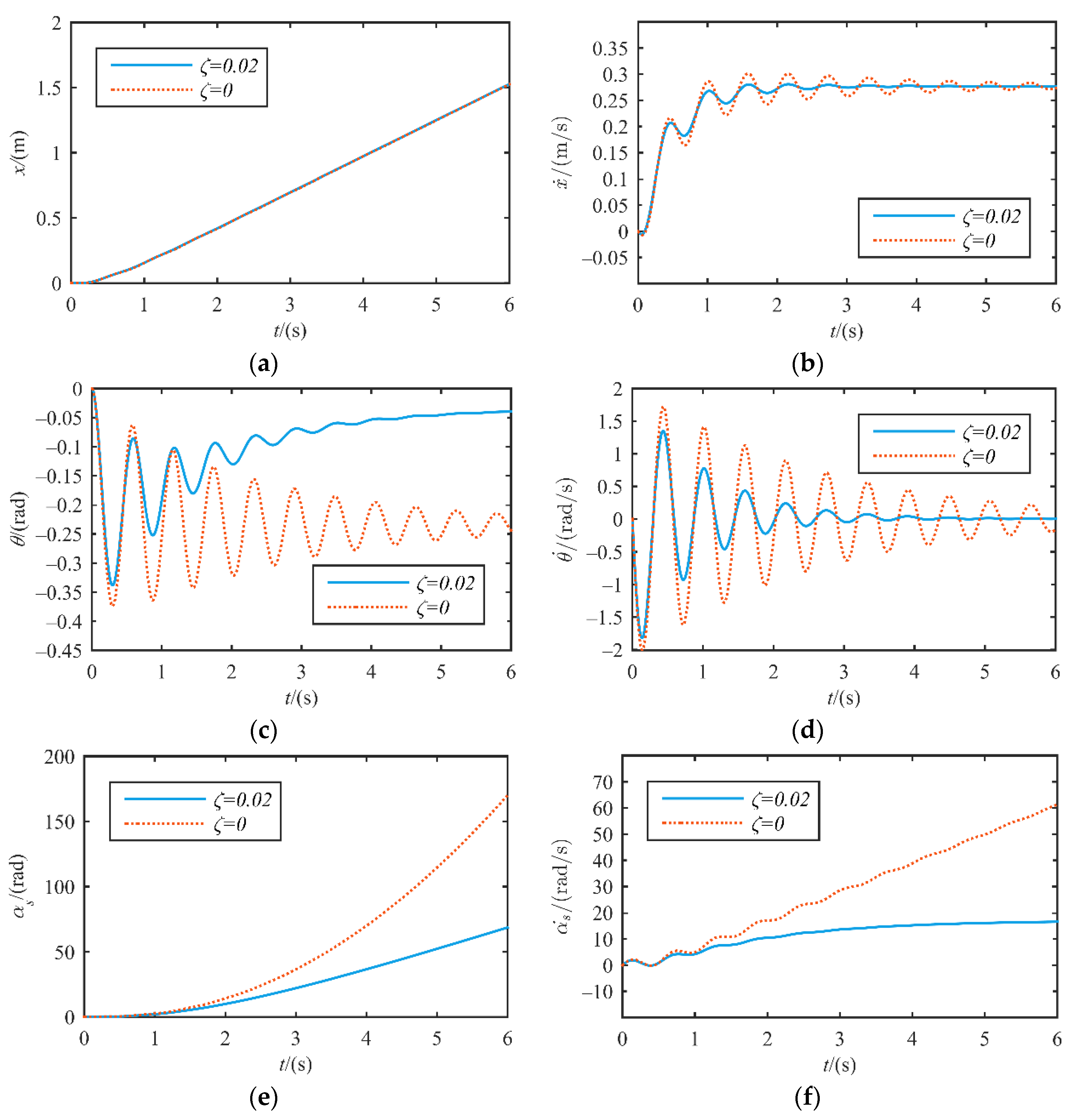
4.1. Simulation

Simulations were carried out in MATLAB in order to reveal characteristics of the dynamic model. The zero-state response under a prescribed input of the rolling motion motor is provided. Parameters used in the simulation are m s = 1.6   kg , m p = 2   kg , m r = 2.2   kg , ζ = 0.02 , l O A = 0.08   m , I s Y Y = 0.0308   kg · m 2 , I p Y Y = 0.00053   kg · m 2 , I r Y Y = 0.0045   kg · m 2 , τ l = 0.4   Nm , τ r = 0   Nm , C L max = 0.92 , C D max = 1.12 , respectively. The frictional resistance exerted on the spherical shell is R f = 0.04   N when the equivalent velocity is set as V e q u = 0.4   m / s .
The time-varying states of those three generalized coordinates are shown in Figure 7.
The simulation results show that the linear velocity of the robot x ˙ , the angle of the IDU platform θ and the angular velocity of the spherical shell α ˙ s proceed to a prescribed value in an oscillation manner as time increases, while the angular velocity of the IDU platform θ ˙ oscillates and then attenuates to zero; the travel distance x increases in a nearly linear manner, when ζ = 0.02 . If ζ = 0 , oscillation will be magnified for x ˙ , θ , θ ˙ and α ˙ s , and θ , α s , α ˙ s will have a large amplitude while x keeps the same.
It can be concluded from the simulation results that a steady linear speed can be achieved by increasing the viscous damping between the spherical shell and the IDU platform; moreover, a less oscillating IDU platform can be achieved at the same time, which is favorable in terms of the performance of sensors and cameras mounted on the IDU.
Simulations were carried out to evaluate the effects of two parameters on the robot’s steady-state velocity when operating on the water, i.e., m r and Δ C f , the adjustable rotator mass and the roughness coefficient of the spherical shell. Figure 8a shows the velocity curve when the rotator mass is set as 0.8 m r , m r and 1.2 m r , respectively, while Figure 8b shows the velocity curve when the roughness coefficient is set as 0 R f , 0.5 R f and 1.5 R f , respectively, with m r representing the nominal mass of the rotator and R f the nominal frictional resistance.
The results indicate that, the reduction of the rotator mass to 0.8 m r results in lower steady-state velocity of the robot, while the increase of the rotator mass has no apparent effect. It is observed that, the spherical shell floats upward when the rotator mass is reduced, leading to lower area of fins immersed under water, thereby reducing the forces exerted on the fins, affecting the steady-state velocity.
On the other hand, the spherical shell dives downward when the rotator mass is increased, which leads to larger area of fins immersed under water; however, this effect is found to be less significant, since the water line is approaching the great circle of the spherical shell that parallels to the surface of water. The wetted surface area increases at the same time, leading to increased hydrodynamic forces because it is positively correlated to the wetted surface area.
As a matter of fact, the current value of m r was chosen such that it roughly maximizes the average area of the fin under water, under the condition that the mass of the robot is kept reasonably low, which is the cause of the behavior observed here.
As for the roughness coefficient, it is found that it has no apparent effect, because the proportion of roughness in the hydrodynamic forces is low.

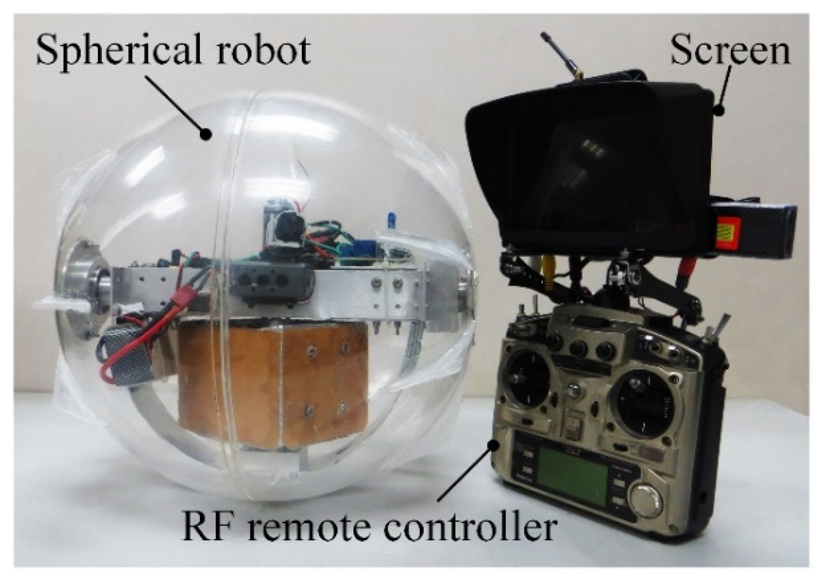
4.2. Amphibious Spherical Robot Prototype

Following the design considerations, an amphibious spherical robot prototype was constructed, as shown in Figure 9. An RF remote controller (Futaba T9CHP) was used to handle the spherical robot remotely.
Some specifications of the amphibious spherical robot prototype are given in Table 1.

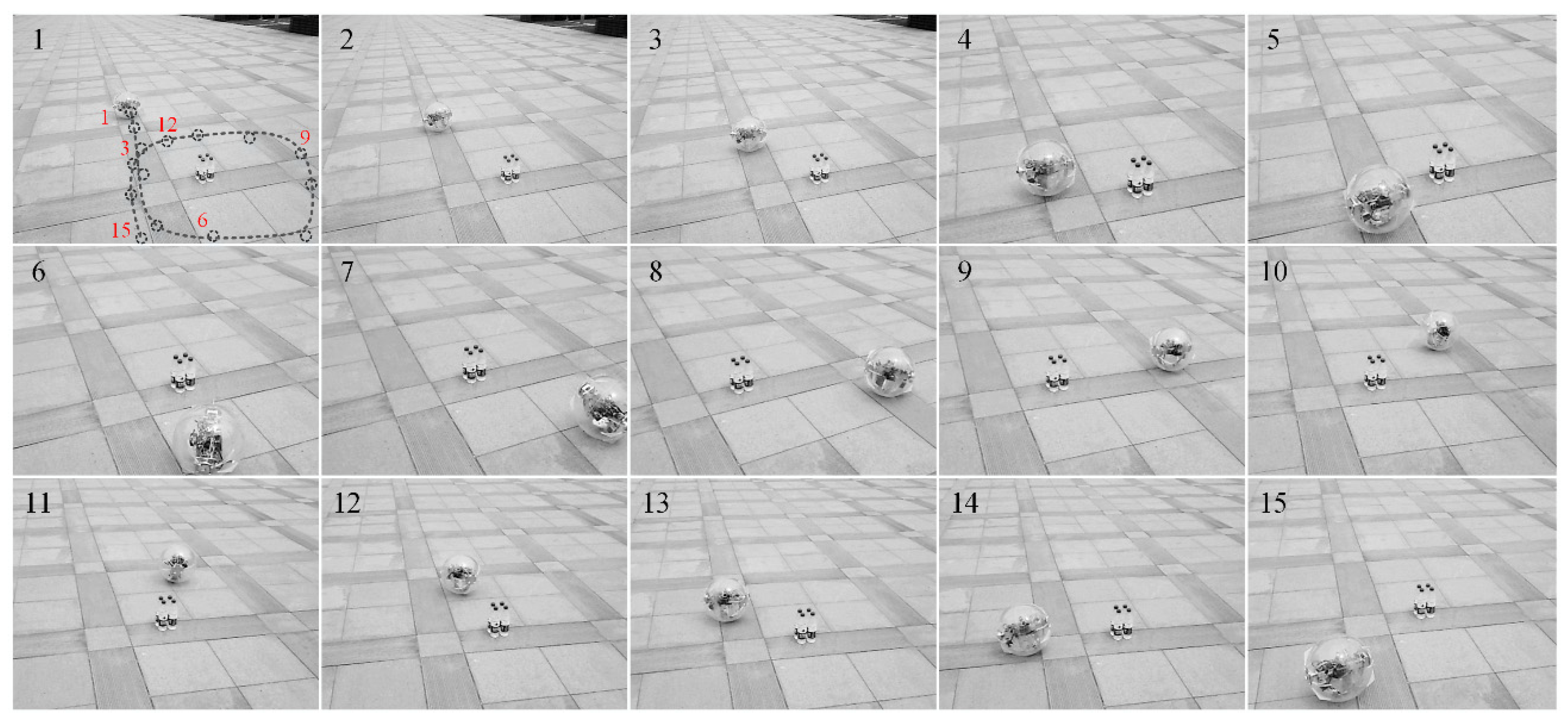
4.3. Movement Experiments

(a)
Movement on Land
Curvilinear motion experiments of the robot were carried out in order to validate its on-land motion capacity, especially its turning capacity without stepping over the fins, as shown in Figure 10. The subgraphs were extracted from a recorded video. The time interval between adjacent subgraphs is 1 s. The robot’s trajectory is shown in the subgraph numbered 1. During the curvilinear motion, the robot steers by spinning the rotator. It was found that, upon limiting the curvature of the trajectory below a threshold, the robot can avoid stepping over the fins when moving on the land.
(b)
Movement on the Water
Linear motion experiments of the amphibious spherical robot on the water were carried out in order to validate the effectiveness of the assistant fins, as shown in Figure 11. Sixteen assistant fins, eight on each hemisphere shell, were attached to the outside surface of the spherical shell. The amphibious spherical robot with fins was then placed onto the surface of static water out of doors. The rolling motion motor was started at t = 0 and the robot’s subsequent track of motion was recorded by a video camera. After that, all the assistant fins were removed from the spherical shell, transforming the amphibious spherical robot to a traditional spherical robot. The linear motion experiment was repeated and the track of motion of the robot without fins was also recorded. Comparison of locomotion performances of those two cases are made based on those video records.
The velocities of the spherical robot with fins and without fins during accelerating process are shown in Figure 12. The results show that the spherical robot with fins speeds up more rapidly than that without fins when accelerating. It takes about 5 s for the spherical robot with fins to reach the velocity of 0.4 m/s, while it takes about 12 s for that without fins to reach the same velocity. The final steady velocity of the spherical robot with fins under constant rolling motion motor outputs, however, is only slightly higher than that without fins. The maximum on-water velocity that this amphibious spherical robot can reach is about 0.4 m/s, which is about 70% of the on-land locomotion velocity.

5. Conclusions

A novel amphibious spherical robot is here proposed for field applications. This amphibious spherical robot’s motion is the composition of the rolling motion based on unbalancing a ballast and the spinning motion based on the principle of conservation of angular momentum. The architecture of the robot is proposed, along with its kinematics and dynamics analyses, which laid out the foundation of manipulation and control of the robot. Moreover, assistant fins are attached on the outside of the spherical shell to increase the propulsion force for the rolling motion, overcoming the disadvantage that a spherical shell slides easily on the surface of water. Results show that the robot with fins speeds up faster than that without fins. With the advantages of high adaptability and robustness, this amphibious spherical robot is suitable for applications in unstructured wild environments.
Future tasks are to carry out experiments to determine coefficients in the empirical equations, so as to obtain a more precise mathematic model for the robot.

Author Contributions

X.C. and Q.Z. provided the research ideas and the theoretical analysis and wrote the paper. Design and experiments, X.C.; analysis, X.C.; supervision, Q.Z. All authors have read and agreed to the published version of the manuscript.

Funding

This research was supported by the National Natural Science Foundation of China under Grant 50705003.

Institutional Review Board Statement

Not applicable.

Informed Consent Statement

Not applicable.

Data Availability Statement

The data presented in this study are available on request from the corresponding author. The data are not publicly available due to restrictions by the affiliation.

Acknowledgments

The authors gratefully acknowledge Tengfei Chai, Yanqiang Zhao, Pengpeng Sun and Yafeng Song from Beihang University for their assistant in constructing the prototype of the amphibious spherical robot.

Conflicts of Interest

The authors claim that there is no conflict of interests regarding the publication of this article.

References

  1. Prahacs, C.; Saudners, A.; Smith, M.K.; McMordie, D.; Buehler, M. Towards legged amphibious mobile robotics. In Proceedings of the Canadian Engineering Education Association (CEEA), Montreal, QC, Canada, 29–30 July 2004; pp. 2371–5243. [Google Scholar]
  2. Hirose, S.; Yamada, H. Snake-like robots [tutorial]. IEEE Rob. Autom. Mag. 2009, 16, 88–98. [Google Scholar] [CrossRef]
  3. Muthugala, M.A.V.J.; Le, A.V.; Cruz, E.S.; Elara, M.R.; Veerajagadheswar, P.; Kumar, M. A self-organizing fuzzy logic classifier for benchmarking robot-aided blasting of ship hulls. Sensors 2020, 20, 3215. [Google Scholar] [CrossRef] [PubMed]
  4. Takayama, T.; Hirose, S. Amphibious 3D active cord mechanism “HELIX” with helical swimming motion. In Proceedings of the IEEE/RSJ International Conference on Intelligent Robots and Systems, Lausanne, Switzerland, 30 September–4 October 2002; pp. 775–780. [Google Scholar]
  5. Yamada, H.; Hirose, S. Study of a 2-DOF joint for the small active cord mechanism. In Proceedings of the IEEE International Conference on Robotics and Automation (ICRA), Kobe, Japan, 12–17 May 2009; pp. 3827–3832. [Google Scholar]
  6. Crespi, A.; Badertscher, A.; Guignard, A.; Ijspeert, A.J. AmphiBot I: An amphibious snake-like robot. Robot. Auton. Syst. 2005, 50, 163–175. [Google Scholar] [CrossRef] [Green Version]
  7. Ijspeert, A.J.; Crespi, A.; Ryczko, D.; Cabelguen, J.-M. From swimming to walking with a salamander robot driven by a spinal cord model. Science 2007, 315, 1416–1420. [Google Scholar] [CrossRef] [PubMed] [Green Version]
  8. Crespi, A.; Ijspeert, A.J. Online optimization of swimming and crawling in an amphibious snake robot. IEEE Trans. Rob. 2008, 24, 75–87. [Google Scholar] [CrossRef] [Green Version]
  9. Crespi, A.; Karakasiliotis, K.; Guignard, A.; Ijspeert, A.J. Salamandra robotica II: An amphibious robot to study salamander-like swimming and walking gaits. IEEE Trans. Rob. 2013, 29, 308–320. [Google Scholar] [CrossRef] [Green Version]
  10. Kelasidi, E.; Liljeback, P.; Pettersen, K.Y.; Gravdahl, J.T. Innovation in underwater robots: Biologically inspired swimming snake robots. IEEE Rob. Autom. Mag. 2016, 23, 44–62. [Google Scholar] [CrossRef] [Green Version]
  11. Kelasidi, E.; Liljeback, P.; Pettersen, K.Y.; Gravdahl, J.T. Integral Line-of-Sight Guidance for Path Following Control of Underwater Snake Robots: Theory and Experiments. IEEE Trans. Rob. 2017, 33, 610–628. [Google Scholar] [CrossRef] [Green Version]
  12. Georgiades, C.; Nahon, M.; Buehler, M. Simulation of an underwater hexapod robot. Ocean Eng. 2009, 36, 39–47. [Google Scholar] [CrossRef]
  13. Meger, D.; Higuera, J.C.G.; Xu, A.; Giguere, P.; Dudek, G. Learning legged swimming gaits from experience. In Proceedings of the IEEE International Conference on Robotics and Automation (ICRA), Seattle, WA, USA, 25–30 May 2015; pp. 2332–2338. [Google Scholar]
  14. Dudek, G.; Giguere, P.; Prahacs, C.; Saunderson, S.; Sattar, J.; Torres-Mendez, L.-A.; Jenkin, M.; German, A.; Hogue, A.; Ripsman, A.; et al. AQUA: An Amphibious Autonomous Robot. Computer 2007, 40, 46–53. [Google Scholar] [CrossRef]
  15. Sattar, J.; Giguère, P.; Dudek, G. Sensor-based behavior control for an autonomous underwater vehicle. Int. J. Rob. Res. 2009, 28, 701–713. [Google Scholar] [CrossRef]
  16. Boxerbaum, A.S.; Werk, P.; Quinn, R.D.; Vaidyanathan, R. Design of an autonomous amphibious robot for surf zone operation: Part I mechanical design for multi-mode mobility. In Proceedings of the IEEE/ASME International Conference on Advanced Intelligent Mechatronics, Monterey, CA, USA, 24–28 July 2005; pp. 1459–1464. [Google Scholar]
  17. Harkins, R.; Ward, J.; Vaidyanathan, R.; Boxerbaum, A.X.; Quinn, R.D. Design of an autonomous amphibious robot for surf zone operations: Part II-hardware, control implementation and simulation. In Proceedings of the IEEE/ASME International Conference on Advanced Intelligent Mechatronics, Monterey, CA, USA, 24–28 July 2005; pp. 1465–1470. [Google Scholar]
  18. Zhang, S.; Zhou, Y.; Xu, M.; Liang, X.; Liu, J.; Yang, J. AmphiHex-I: Locomotory Performance in Amphibious Environments with Specially Designed Transformable Flipper Legs. IEEE/ASME Trans. Mechatron. 2016, 21, 1720–1731. [Google Scholar] [CrossRef]
  19. Zhong, B.; Zhang, S.; Xu, M.; Zhou, Y.; Fang, T.; Li, W. On a CPG-based hexapod robot: AmphiHex-II with variable stiffness legs. IEEE/ASME Trans. Mechatron. 2018, 23, 542–551. [Google Scholar] [CrossRef] [Green Version]
  20. Chen, Y.; Doshi, N.; Goldberg, B.; Wang, H.; Wood, R.J. Controllable water surface to underwater transition through electrowetting in a hybrid terrestrial-aquatic microrobot. Nat. Commun. 2018, 9, 2495. [Google Scholar] [CrossRef] [PubMed]
  21. Kaznov, V.; Seeman, M. Outdoor navigation with a spherical amphibious robot. In Proceedings of the IEEE/RSJ International Conference on Intelligent Robots and Systems (IROS), Taipei, Taiwan, 18–22 October 2010; pp. 5113–5118. [Google Scholar]
  22. Li, M.; Guo, S.; Hirata, H.; Ishihara, H. Design and performance evaluation of an amphibious spherical robot. Robot. Auton. Syst. 2015, 64, 21–34. [Google Scholar] [CrossRef]
  23. He, Y.; Shi, L.; Guo, S.; Guo, P.; Xiao, R. Numerical simulation and hydrodynamic analysis of an amphibious spherical robot. In Proceedings of the IEEE International Conference on Mechatronics and Automation, Beijing, China, 2–5 August 2015; pp. 848–853. [Google Scholar]
  24. Li, Y.; Yang, M.; Sun, H.; Liu, Z.; Zhang, Y. A Novel Amphibious Spherical Robot Equipped with Flywheel, Pendulum, and Propeller. J. Intell. Rob. Syst. 2018, 89, 485–501. [Google Scholar] [CrossRef]
  25. Tadakuma, K.; Tadakuma, R.; Aigo, M.; Shimojo, M.; Higashimori, M.; Kaneko, M. “Omni-Paddle”: Amphibious spherical rotary paddle mechanism. In Proceedings of the IEEE International Conference on Robotics and Automation, Shanghai, China, 9–13 May 2011; pp. 5056–5062. [Google Scholar]
  26. Zhan, Q.; Cai, Y.; Yan, C. Design, analysis and experiments of an omni-directional spherical robot. In Proceedings of the IEEE International Conference on Robotics and Automation, Shanghai, China, 9–13 May 2011; pp. 4921–4926. [Google Scholar]
  27. Cai, Y.; Zhan, Q.; Xi, X. Path tracking control of a spherical mobile robot. Mech. Mach. Theory 2012, 51, 58–73. [Google Scholar] [CrossRef]
  28. Tupper, E.C. Introduction to Naval Architecture; Butterworth-Heinemann: Jersey City, NJ, USA, 2013. [Google Scholar]
  29. White, F.M. Fluid Mechanics, 4th ed.; McGraw-Hill Higher Education: Boston, MA, USA, 1998. [Google Scholar]
  30. Morsi, S.A.; Alexander, A.J. An investigation of particle trajectories in two-phase flow systems. J. Fluid Mech. 1972, 55, 193–208. [Google Scholar] [CrossRef]
  31. Cheng, C.M.; Fu, C.L. Characteristic of wind loads on a hemispherical dome in smooth flow and turbulent boundary layer flow. J. Wind Eng. Ind. Aerodyn. 2010, 98, 328–344. [Google Scholar] [CrossRef]
  32. Healey, A.J.; Rock, S.M.; Cody, S.; Miles, D.; Brown, J.P. Toward an improved understanding of thruster dynamics for underwater vehicles. IEEE J. Ocean Eng. 1995, 20, 354–361. [Google Scholar] [CrossRef]
Figure 1. Mechanical structure of the amphibious spherical robot.
Applsci 11 03739 g001
Figure 2. Schematic of rolling motion and spinning motion.
Applsci 11 03739 g002
Figure 3. Schematic of electrical actuation and control system.
Applsci 11 03739 g003
Figure 4. Control block diagram of the robot.
Applsci 11 03739 g004
Figure 5. Coordinate frames of the robot.
Applsci 11 03739 g005
Figure 6. Force analysis of the amphibious spherical robot.
Applsci 11 03739 g006
Figure 7. Time-varying states of the generalized coordinates. (a) Travel distance of the robot; (b) Speed of the robot; (c) Angle of the IDU platform; (d) Angular velocity of the IDU platform; (e) Angle of the spherical shell; (f) Angular velocity of the spherical shell.
Applsci 11 03739 g007
Figure 8. The velocity curve of the robot under different parameters. (a) Different rotator masses, (b) Different roughness coefficients of the spherical shell.
Applsci 11 03739 g008
Figure 9. Amphibious spherical robot prototype.
Applsci 11 03739 g009
Figure 10. Curvilinear motion on land.
Applsci 11 03739 g010
Figure 11. Movement on the water. (a) Fins attached; (b) Fins removed.
Applsci 11 03739 g011
Figure 12. Velocities of the spherical robot with fins and without fins.
Applsci 11 03739 g012
Table 1. Specifications of the amphibious spherical robot.
ItemsParameters
Diameter350 mm
Weight5.8 kg
Power supply voltage24 V
Duration time1 h
Speed (on ground)0.6 m/s
Speed (on the water)0.4 m/s(16 fins)
Control signal transmitting distance500 m
Camera signal transmitting distance60 m
Publisher’s Note: MDPI stays neutral with regard to jurisdictional claims in published maps and institutional affiliations.

