Path Planning Based on Obstacle-Dependent Gaussian Model Predictive Control for Autonomous Driving

Abstract

Path planning research plays a vital role in terms of safety and comfort in autonomous driving systems. This paper focuses on safe driving and comfort riding through path planning in autonomous driving applications and proposes autonomous driving path planning through an optimal controller integrating obstacle-dependent Gaussian (ODG) and model prediction control (MPC). The ODG algorithm integrates the information from the sensors and calculates the risk factors in the driving environment. The MPC function finds vehicle control signals close to the objective function under limited conditions, such as the structural shape of the vehicle and road driving conditions. The proposed method provides safe control and minimizes vehicle shaking due to the tendency to respond to avoid obstacles quickly. We conducted an experiment using mobile robots, similar to an actual vehicle, to verify the proposed algorithm performance. The experimental results show that the average safety metric is 72.34%, a higher ISO-2631 comport score than others, while the average processing time is approximately 14.2 ms/frame.

1. Introduction

Autonomous driving refers to a technology that determines the driving situation through sensors and drives to the destination without driver intervention. Autonomous driving in the future is expected to increase traffic efficiency and driver convenience, and enhance traffic safety. Most traffic accidents and fatalities occur during lane changes and overtaking [1]. Such accidents greatly injure human life, and autonomous driving remains an important task for full commercialization in the current technology regarding path planning safety. Adaptive cruise control [2], lane-keeping assist [3], and automated emergency braking [4] of advanced driver assistance systems (ADAS) technologies have positive effects on driving safety [5]. Recently, Advanced driver assistance systems (ADAS) use advanced detection sensors, global positioning systems (GPS), and video equipment to recognize situations while driving, judge the situation, and control the car. Therefore, companies, such as Google and Tesla, are working on fully autonomous driving without human intervention [6]. However, it is still difficult to research the technology of fully autonomous driving. Therefore, this paper suggests determining how a vehicle should behave concerning surrounding vehicles as an obstacle avoidance path planning problem.

Path planning is a technology that enables mobile robots or vehicles to move autonomously. With the advancement of technology, research on avoiding obstacles without human intervention has been actively conducted in the field of autonomous driving [7]. The path planning research area is divided into global path planning, which generates a path using the information from the entire map, and local path planning, which generates a path using sensors. Global path planning is a low-resolution high-level planning that determines the map information before the vehicle runs, creates a path, and then operates. Frequently used global path planning algorithms include sampling-based approaches [8], search-based approaches [9], continuous geometric curve-based methods [10], and artificial dislocation field approaches [11].

The sampling-based approach is a method that quickly searches the space by selecting a random point in each sample and creating a path continuously by extending it in the random point direction. Because the algorithm relaxes the completeness requirement, it has the advantage of being able to relatively quickly find a path that is possible from the start to the target point, even with a high-dimensional state space. Therefore, the destination can be reached safely without problems at a local minimum based on probability. The Rapidly exploring Random Tree (RRT) and RRT* algorithms [8] are typical examples of the sampling-based approach method. However, the sampling-based approach methods have a limitation in finding the best path: the disadvantage of unnecessary costs in computation and inefficiency.

The second method is the search-based approach method. The biggest feature of this algorithm is searching for a heuristic-based search as the graph-based method. After the graph is generated, the path is searched from the start to the target point at the minimum cost. The optimum path can be found faster using the correct heuristic function. Examples include the Dijkstra algorithm and A* algorithm [9]. However, the computation amount is limited due to the large graph and complexity of the environment. If the environment changes after determining the shortest path, it is difficult to respond quickly. Therefore, the algorithm works well in low-speed applications but has a limitation in high-speed driving.

The third method, the continuous geometry curve-based method, is an optimized path planning algorithm that uses the spline function used in various mobile robot fields. The search and sample methods described above do not include vehicle dynamics; thus, optimal path planning cannot be performed. However, this method is based on vehicle dynamics and many studies on path smooth algorithms [12]. For example, the continuous geometry curve-based method can be performed using spline curves [13], bezier curves [14], and polynomial curves [15]. However, these methods also have a limitation because they do not perform optimal path planning in terms of relative speed.

The fourth method is the risk-based approach, which consists of repulsive forces to avoid collision and attractive forces to reach the goal. Therefore, when accurate information on the roads and surrounding obstacles is available to recognize, it is an effective method to generate a trajectory without causing an obstacle collision. Because the risk-based approach method does not contain vehicle dynamics, it cannot guarantee experimentation in real vehicles. Examples include the artificial potential field (APF) [11], which updates the peripheral information in the driving conditions of the expressway; then, the algorithm works. There are also attempts to imitate a way of the person as a way of defining risk, such as Driver’s Risk Field [16] and humans motor response [17]. While theses approaches to path planning through obstacle avoidance provide good results in many applications, there are some major drawbacks to the trade-off between essential computational resources and solution optimization. Many of the commonly used path planning methods rely heavily on extensive simulation testing because there is no formal stability analysis and verification methodology.

Therefore, it is desirable to formalize the path planning problem as a low complexity problem. In the Model Predictive Control (MPC) path planning, a path is found to solve a constrained optimal control problem over a finite time horizon. A cost function is minimized subject to constraints, including vehicle dynamics, design and physical constraints, and additional constraints introduced to avoid collision with surrounding vehicles. The constrained optimal control problem is solved in the receding horizon, i.e., at every time step, the problem is formulated over a shifted time horizon based on newly available sensor measurement information. The main advantage of resorting to such a formulation is that collision avoidance is guaranteed, provided that the optimization problem is feasible. However, collision avoidance constraints for trajectory planning are generally non-convex, limiting the feasibility and uniqueness of the solution to the optimization problem. Researchers rely on techniques such as piecewise-linear model [18], Gaussian process-based approach [19], convexification [20], and machine learning [21,22,23] to address the issue.

Local path planning is a high-resolution low-level planning that operates by generating a path using a limited time and space boundary [24]. These algorithms make a finite set of trajectories that follow a waypoint provided by a global path planner, avoiding obstacles detected by the sensor. The discrete scheme of this trajectory is optimized by the integration of differential equations in vehicle dynamics [25]. Typically, the bug algorithm, a local path planning algorithm, works based on sensors without information on the map [26]. These algorithms make a straight line in the direction of the target point provided by the global path planner and then move along the line and encounter an obstacle. The algorithm detects the obstacle and moves around it. After moving around it, the algorithm finds the nearest point to the target point and moves back to the target point.

Another example of local path planning is the tentacle method [27]. This method creates a path by selecting only one of several vehicle trajectories depending on the obstacle location and uses the local path planning method for global path planning. Because this method does not consider moving people or moving vehicles, it is currently used as path smoothing.

The aforementioned global path planning method limits the information from the entire map in the outdoor case where the map information is needed. The concept of local path planning is required to compensate for the limitations of global path planning [24]. In most autonomous driving currently under research, maps are created through sensors. Then, path planning is conducted without information on the entire map. Many current path planning studies have used global path planning as local path planning [28,29,30,31]. Therefore, this paper focuses on the local path planning method of autonomous vehicles based on a predefined global path.

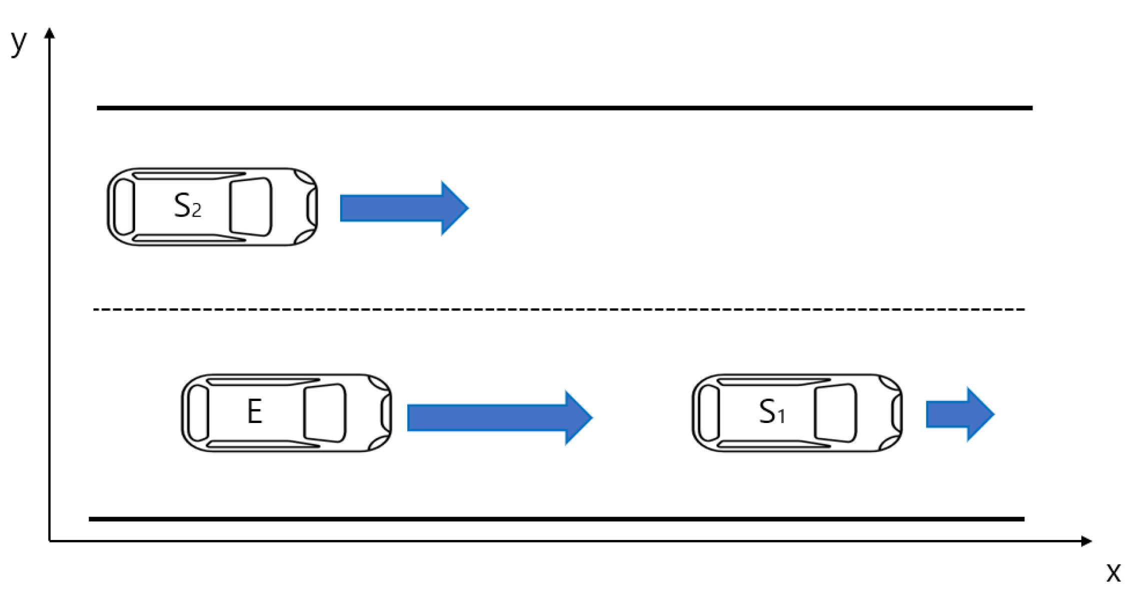
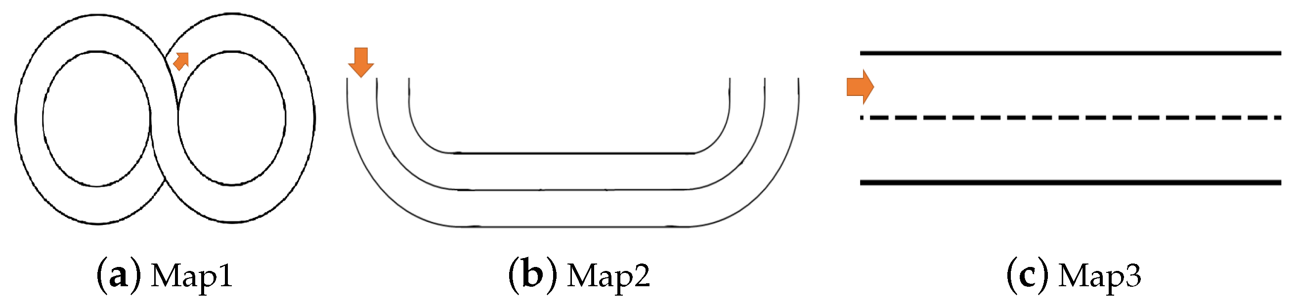
Autonomous driving requires the ability to maintain lanes and speed while overtaking front vehicles. In the driving environment, lanes are divided into solid lines and dotted lines, as shown in Figure 1. The Ego vehicle E must be controlled to avoid a dangerous collision with the surrounding vehicle $S_k(k=1,\cdots ,q)$, where q is the number of surrounding vehicles.

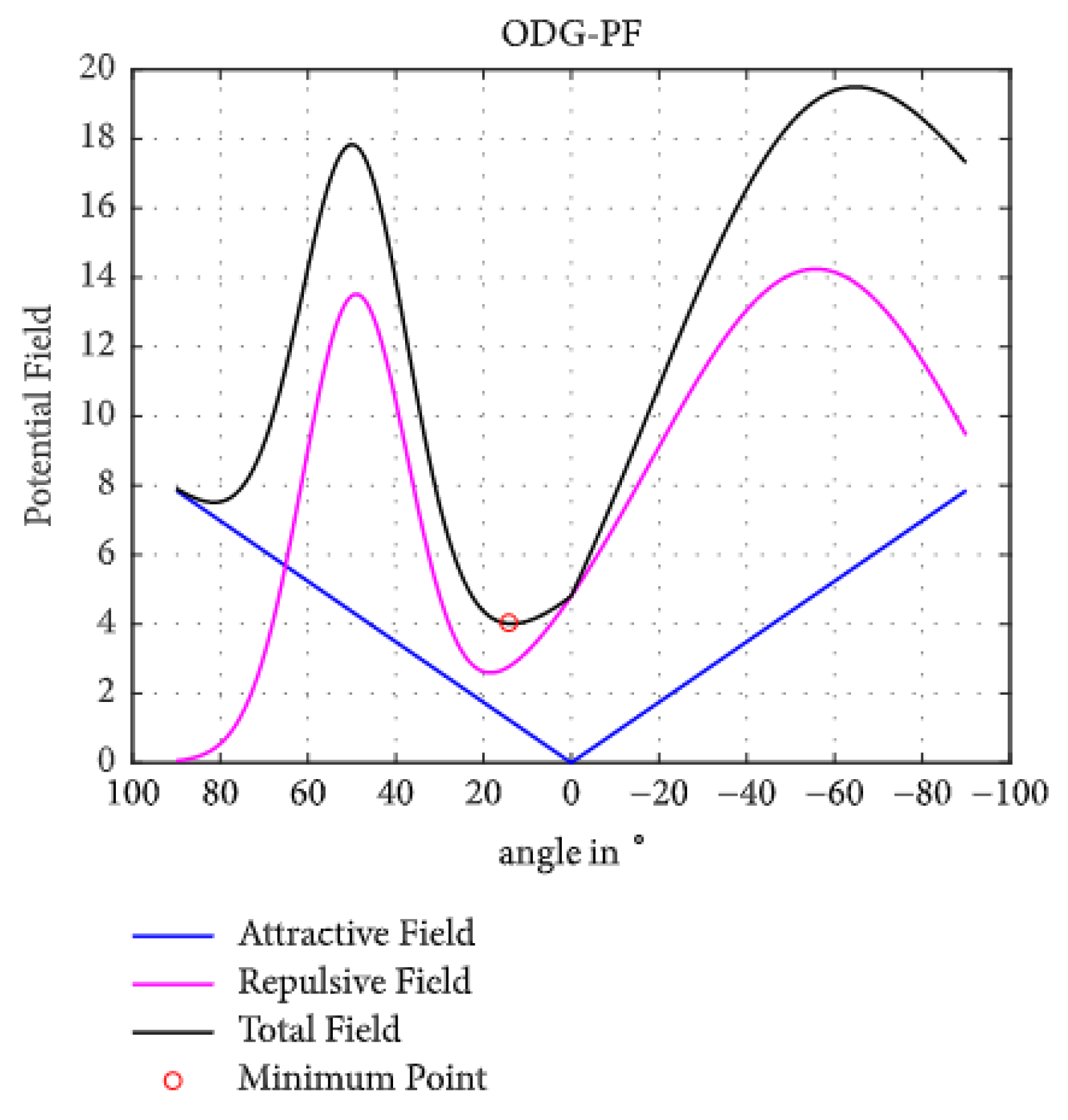
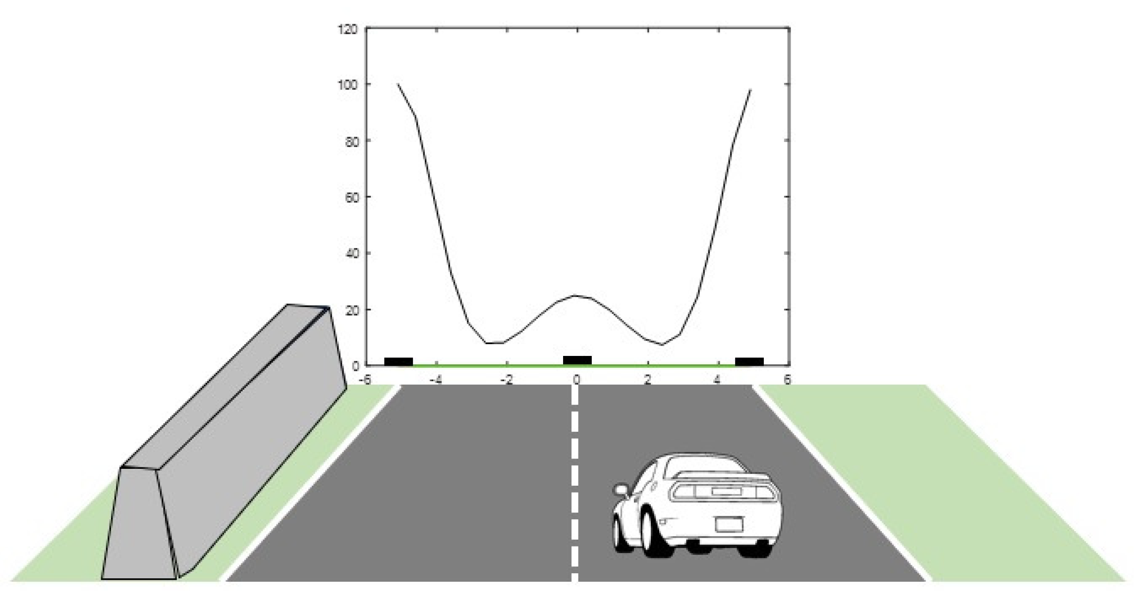
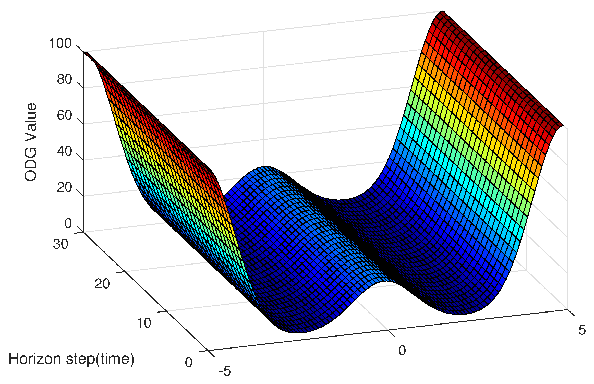
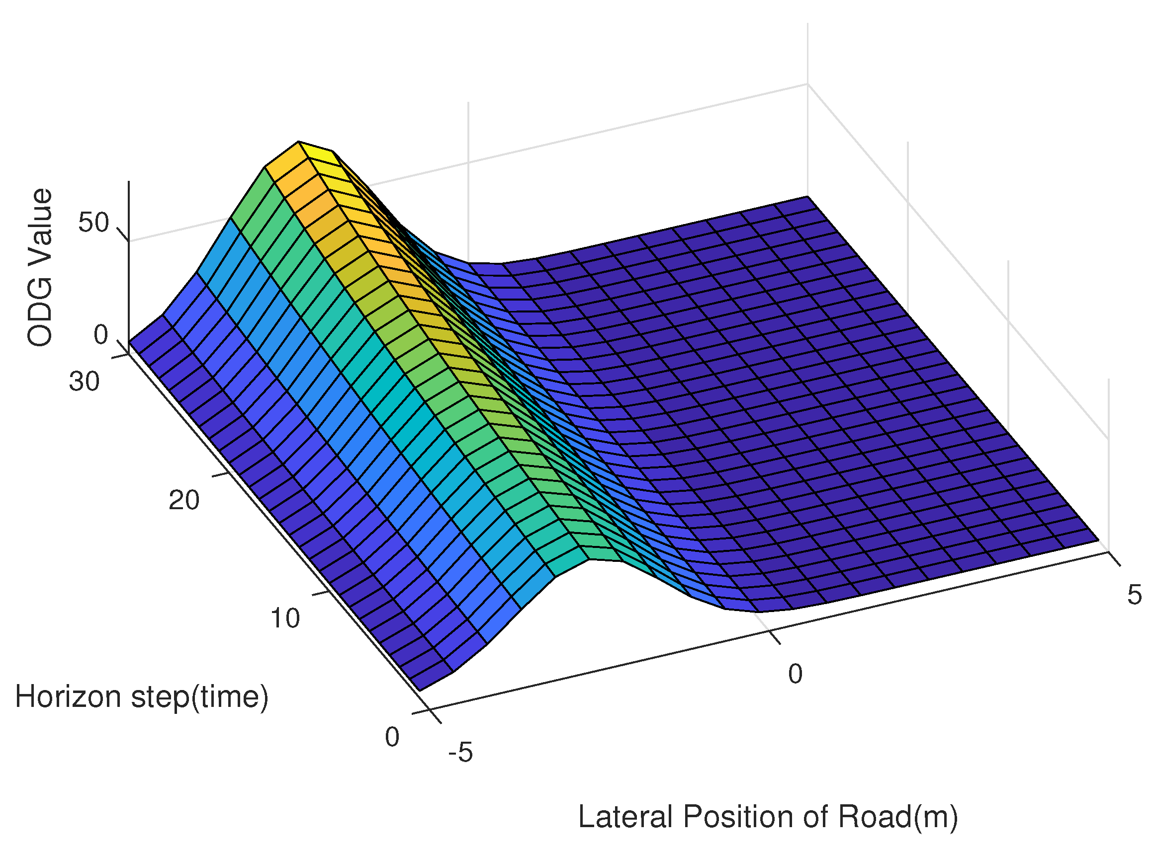
The APF algorithm [32] described in Section 1 explains the results of effectively conducting path planning with attractive and repulsive forces differently from other algorithms. However, due to the many parameters used for control, it is difficult to determine the optimal control. Thus, Cho et al. [33] experimented using the ODG potential field (PF), the improved version of the APF algorithm. The ODG PF algorithm uses the Obstacle-Dependent Gaussian (ODG) model, which expresses the presence of an obstacle measured by the sensor as a risk using a Gaussian function [33]. It is confirmed that path planning is more stable than APF through the experiment while having fewer parameters. However, as the ODG PF does not contain vehicle dynamics, the experimental results show unstable control, which is limited in real vehicle models.

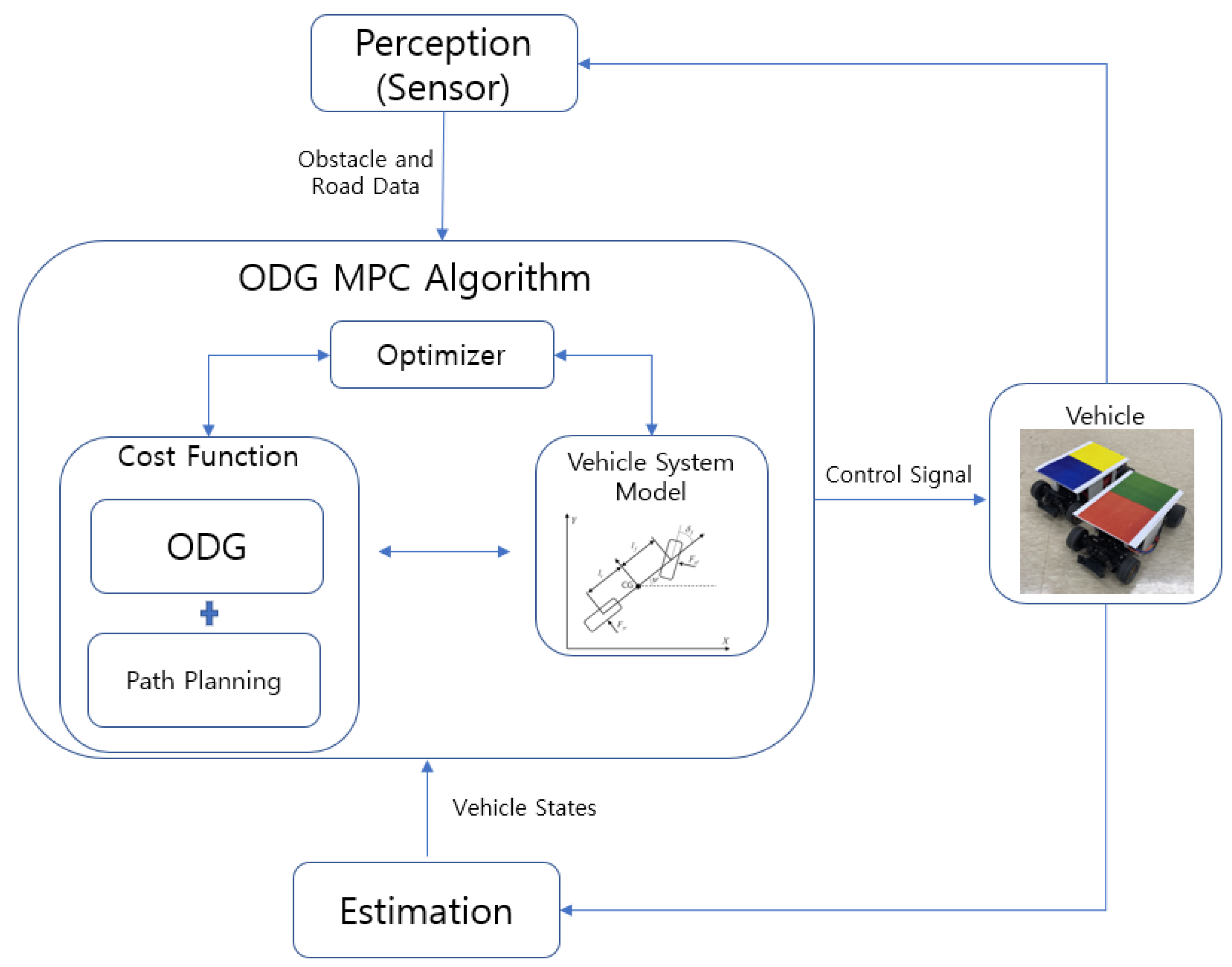
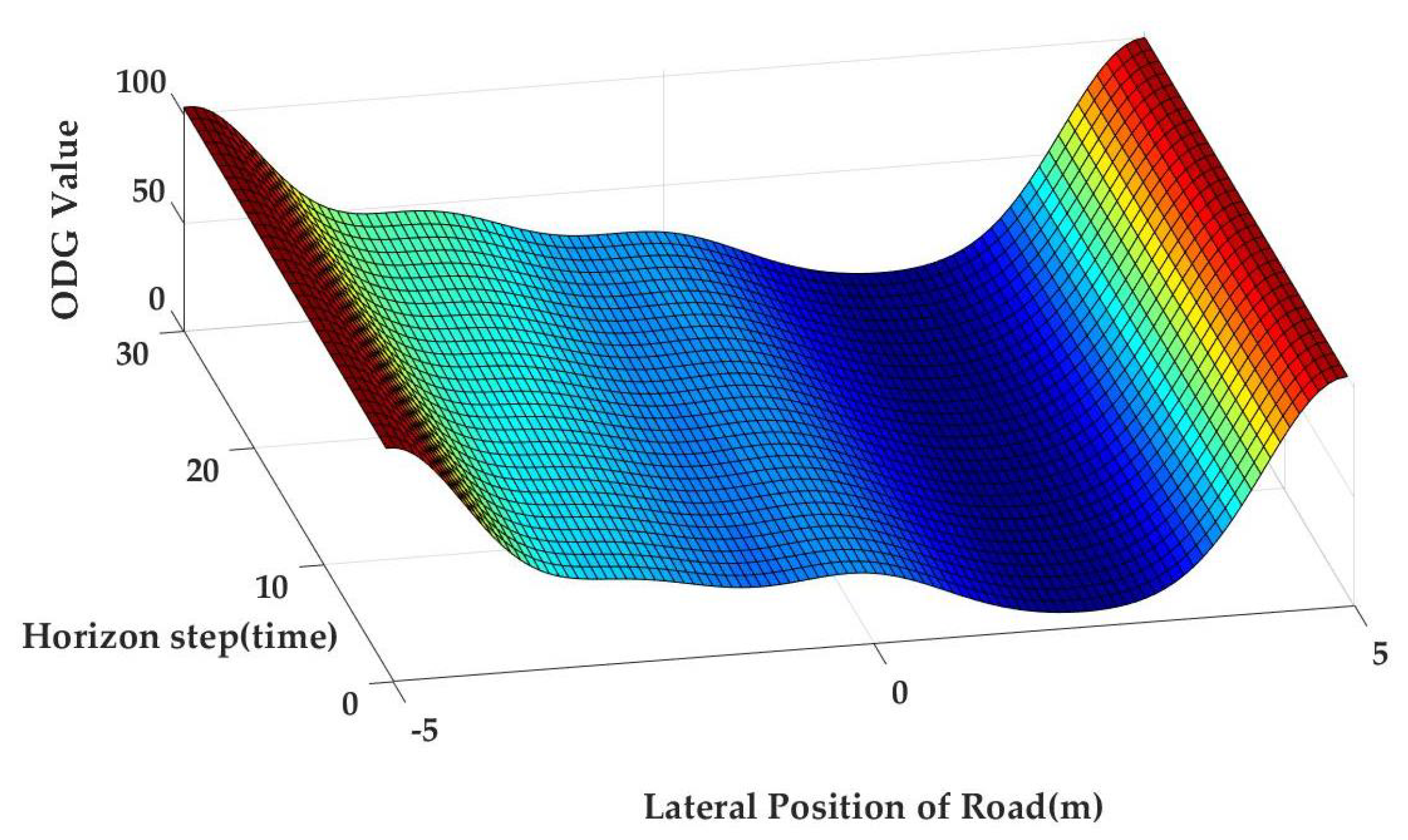
We propose a risk model-generalized ODG model to create a path that incorporates the vehicle risk rather than removing the MPC constraints on collision avoidance. The proposed algorithm calculates the optimal path using MPC, and in this process, the cost function includes the proposed risk model that expresses the risk information of the obstacle detected by the sensor. Due to the characteristics of the proposed algorithm, it tends to react quickly to obstacle information detected by the sensor and avoid the obstacle. As a result, stable driving is possible with a quick response to an obstacle vehicle, and a quick response creates a low lateral acceleration. Therefore, we propose an optimal controller that integrates the proposed risk model and MPC to solve the computational problem and enable stable obstacle avoidance path planning. The main contributions of this paper are as follows:

(1)

We proposed a general ODG-based risk model to apply for vehicles and lanes to define the risk of driving.

(2)

We combined the general ODG-based risk model and MPC, and the proposed algorithm responds to avoid obstacles quickly. Due to this tendency, the proposed method provides safe control and minimizes vehicle shake.

(3)

The proposed method can control the vehicle for the obstacle avoidance process in real-time, and it has been confirmed through experiments.

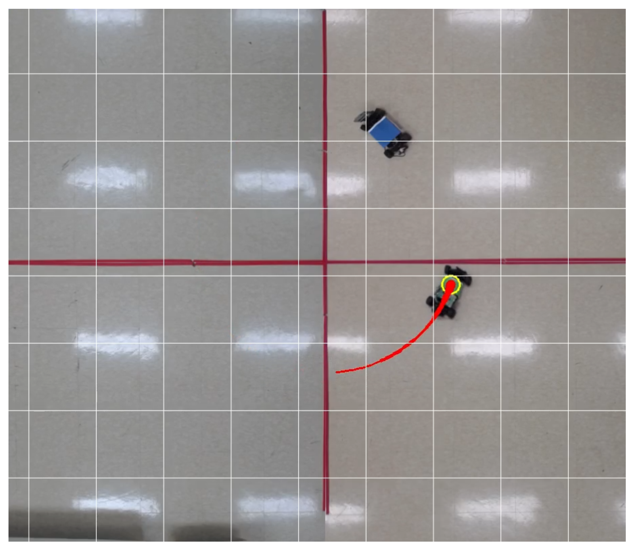
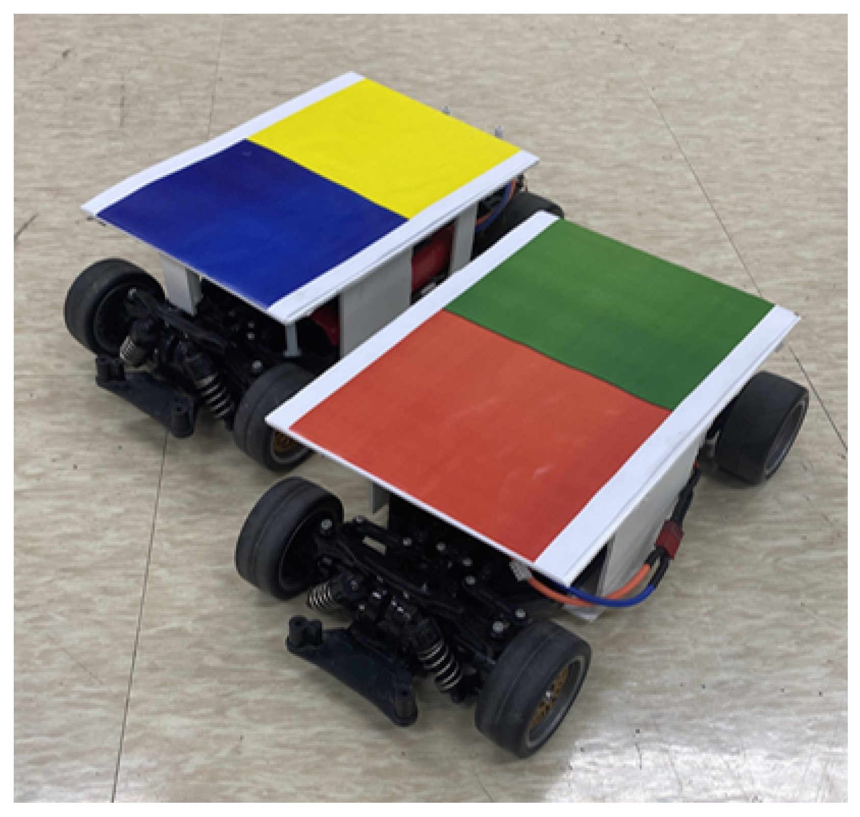
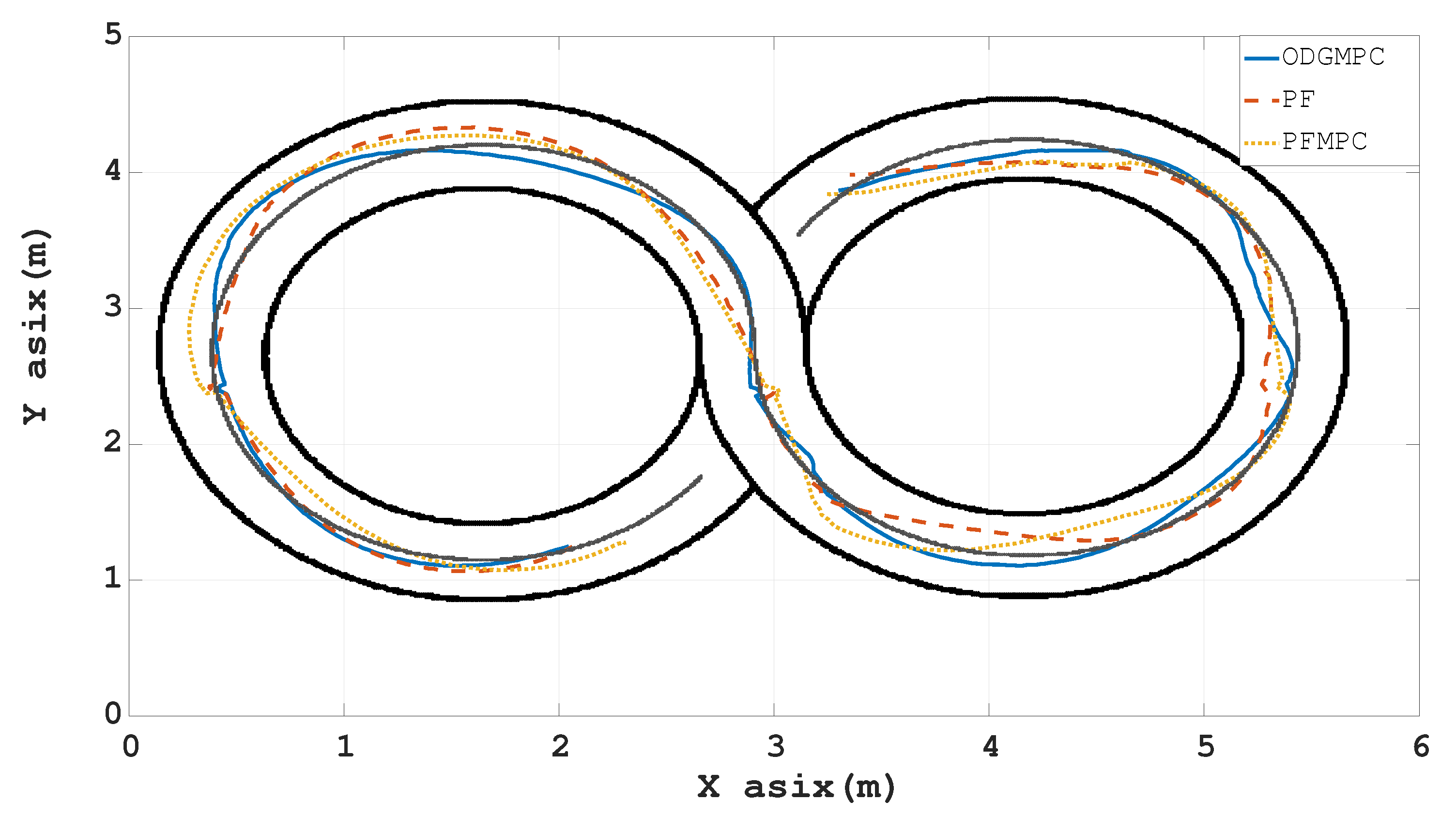
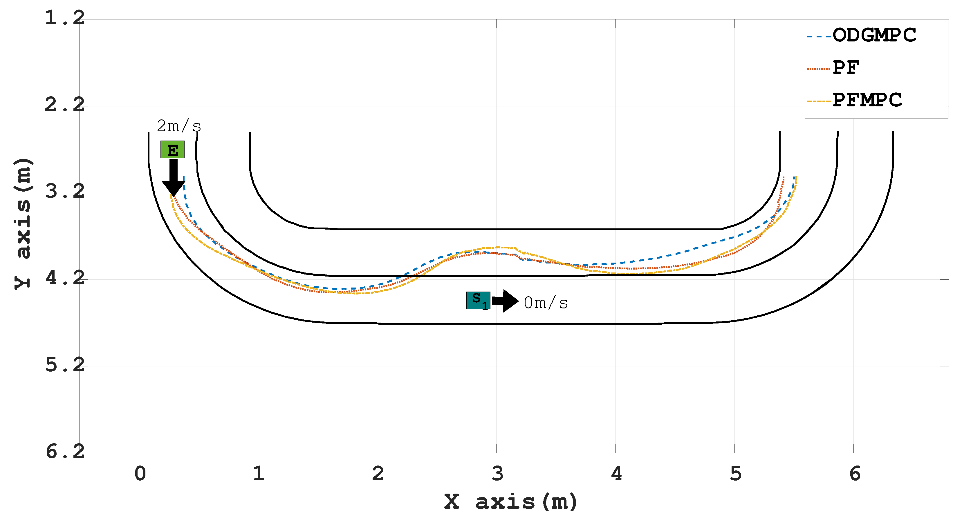
This paper is organized as follows. Section 2 discusses related work, introducing the ODG model and the MPC function. Section 3 defines the proposed method using the proposed risk model and MPC. Section 4 presents an experiment using mobile robots similar to vehicle dynamics and the experimental results of propose method. Section 5 summarizes and concludes. In addition, the nomenclature and variable definition are given in Nomenclature, respectively.

2. Related Work

Before describing the proposed algorithm, this section briefly reviews the fundamental theories associated with the proposed algorithm. We first describe the ODG PF algorithm and the MPC function. Section 2.1 describes the ODG PF algorithm, and Section 2.2 describes the MPC function.

2.1. Obstacle-Dependent Gaussian Potential Field Algorithm

This section describes a risk-based algorithm, ODG PF. Cho et al. [33] found that the laser range finder (LRF) sensor data measured in the LRF sensor are used to determine obstacles and measure the risk using the Gaussian function at the measured value. Using the measured risk, move the yaw angle of the vehicle through the inertial measurement unit sensor to a place with low risk.

The received data are measured in Figure 2, and the measured data are listed in Figure 3. As a result, the measured data determine the obstacle [33]. Figure 4 stands for the enlargement of the angle occupied by the obstacle after considering the vehicle width. The ODG PF algorithm measures the width for the determined obstacle, as depicted in Figure 4, and calculates the repulsive field for the measured obstacle. Thus, for $\theta$ measured for each obstacle in the sensor, as presented in (1), the Gaussian function is calculated to produce a reactive field:

$$f_{rep}({\theta }_i)=\sum _{k=1}^n{k}_{rep}exp(-\frac{{({\theta }_k-{\theta }_i)}^2}{2{\sigma }_k^2}).$$

(1)

$$k_{rep}=(d_{max}-d_k)exp(\frac{1}{2}),$$

(2)

where ${\theta }_k$ is a center angle of each obstacle, $d_{max}$ is the maximum detection range, ${\sigma }_k$ denotes half of the angle occupied by the kth obstacle, and n is the number of obstacles. In ${\theta }_i$, ith indicates the data contract of the sensor data (i = 1, ..., 361), and it means the sequence number of the approach angle. The coefficient $k_{rep}$ is set up for each obstacle to embrace the Gaussian likelihood for each obstacle fully.

$$f_{att}({\theta }_i)=k_{att}\left|{\theta }_{goal}-{\theta }_i\right|,$$

(3)

$$f_{total}({\theta }_i)=f_{rep}({\theta }_i)+f_{att}({\theta }_i),$$

(4)

where $k_{att}$ is the weight parameter for an attractive field. The attractive field is calculated to follow the direction of the goal point (${\theta }_{goal}$), as shown in (3). Thus, the total fields are available, as presented in (4). When the total field is obtained, the vehicle is moved by the $\theta$ of the minimum point, as depicted in Figure 5.

2.2. Model Predictive Control

This section describes the MPC function, as described in [29,30]. The MPC algorithm finds the optimal control to minimize the cost function that satisfies the constraints consisting of the predicted horizon and system model [29,30]. Therefore, as depicted in Figure 6, the MPC algorithm is a way to predict status variables or outputs using models of control targets. This method can provide optimized control using appropriate cost functions and constraints.

The MPC method [29,30] has the advantage that it can control a set of target points in the constrained system. If the target’s steady state is not admissible, Limon et al. [29] induced the system into an acceptable safe state. The rest of this section describes how to implement the MPC algorithm.

The discrete-time LTI system is given by (5). Moreover, $x\in {\mathrm{I}\mathrm{R}}^{n_x}$ denotes the state, and $u\in {\mathrm{I}\mathrm{R}}^{n_u}$ denotes the input vector. The variable A indicates the system matrix, and B is the input matrix:

$$x(k+1)=Ax(k)+Bu(k),$$

(5)

where $A\in {\mathrm{I}\mathrm{R}}^{n_x\times n_x}$ and $B\in {\mathrm{I}\mathrm{R}}^{n_x\times n_u}$. The constraints are expressed in (6):

$$z={(x^{\mathrm{T}},u^{\mathrm{T}})}^T\in Z\stackrel{\Delta }{=}\{z\in {\mathrm{I}\mathrm{R}}^{n_x+n_u}:A_{z}z\le b_z\},$$

(6)

where $\mathrm{Z}$ is a nonempty compact convex polyhedron set containing the origin in its interior, and $A_z\in {\mathrm{I}\mathrm{R}}^{n_z\times (n_x+n_u)},b_z\in {\mathrm{I}\mathrm{R}}^{n_z},n_z$ denotes the number of constraints. The inputs of the system in (5) and the subspace of the steady states have a linear representation in the following form:

$$z_{ss}=M_{\theta }\theta ,$$

(7)

where $z_{ss}^{\mathrm{T}}=(x_{ss}^{\mathrm{T}},u_{ss}^{\mathrm{T}})$ is the stack of the steady-state solution of (5), and $x_{ss}$ is obtained by applying the control action $u_{ss}$ to the system in (5). In addition, $\theta \in {\mathrm{I}\mathrm{R}}^{n_{\theta }}$ is the parameter vector, and $M_{\theta }$ is a matrix of suitable dimensions. In accordance with the works in [29,30], the objective is to find a control of the form $u=f_N(x(k),\widehat{x})$ such that it minimizes the cost function subject to the system constraints. Equation (5) is controlled to the target state while fulfilling the constraints in (6). Furthermore, with N being the prediction horizon, the function map $u=F_N(x(k),\widehat{x})$ can be calculated by solving the following optimization problems parameterized in x and $\widehat{x}$. The optimization problem of (8) can be solved by expressing it as a quadratic programming problem [29,30].

$$\begin{array}{c}\underset{u_i,\theta }{min}{J}_N(u,\theta ,x,\widehat{x})\hfill \\ subjectto\hfill \\ x_0=x(0),\hfill \\ x(i+1)=Ax(i)+Bu(i),i=0,1,...,N-1\hfill \\ {(x_{ss}^{\mathrm{T}},u_{ss}^{\mathrm{T}})}^T=M_{\theta }\theta ,\hfill \\ {({x_N}^{\mathrm{T}},{\theta }^{\mathrm{T}})}^T\in X_f^g,\hfill \end{array}$$

(8)

where the terminal set $X_f^g$ is chosen as follows:

$$X_f^g=\left\{{(x^{\mathrm{T}},{\theta }^{\mathrm{T}})}^T\in {\mathrm{I}\mathrm{R}}^{n_x+n_{\theta }}:(x,Kx+L\theta )\in Z,M_{\theta }\theta \in Z\right\},$$

(9)

with $K\in {\mathrm{I}\mathrm{R}}^{n_u\times n_x}$ being a constant matrix such that the eigenvalues of $A+BK$ lie within the unit circle [29,30]. Therefore, the cost function $J_N(u,\theta ,x,\widehat{x})$ is chosen as follows:

$$J_N(u,\theta ,x,\widehat{x})=\sum _{i=0}^N[{∥x(i)-x_{ss}∥}_Q^2+{∥u(i)-u_{ss}∥}_R^2]+{∥x(N)-x_{ss}∥}_P^2+{∥x_{ss}-\widehat{x}∥}_T^2,$$

(10)

where u and $\theta$ are division variables that solve the optimization problem of (8), and $Q=Q^{\mathrm{T}}>0,R=R^{\mathrm{T}}>0,T=T^{\mathrm{T}}>0,P=P^{\mathrm{T}}>0$, which define the appropriate dimensions. The optimal control action is applied using the required horizon strategy $f_N(x,\widehat{x})=u^{*}(0)$, where $u^{*}(0)$ indicates the first element of the optimal sequence. Therefore, we can control the vehicle to approach the desired state by defining MPC, and we confirmed that the path could be found using the Gaussian function for obstacles in the ODG PF algorithm and that the vehicle could follow the path using the MPC algorithm.

3. Real-Time Obstacle-Dependent Gaussian Model Prediction Control Algorithm

In this section, we explain the ODG MPC algorithm. As illustrated in Figure 7, we designated a path to avoid obstacles using the ODG MPC algorithm and vehicle model. The proposed autonomous driving system consists of a controller, perception, estimation, and a vehicle. First, the camera data are integrated to obtain information on the vehicle location, vehicle speed, and roadway obstacle information. The control signal is sent to the vehicle for stable movement using an algorithm incorporating the ODG and MPC algorithm through the information obtained from the perception from the ODG MPC algorithm and the vehicle states via the estimation.

The ODG MPC algorithm includes three basic elements, which we detail in this section:

• vehicle dynamic modeling,
• ODG algorithm, and
• path planning.

3.1. Vehicle Dynamic Modeling

We mark the notation with the bicycle model, as illustrated in Figure 8. The MPC models of host vehicles can be expressed in a state-space equation. As in [34], we used the 2-degrees of freedom (DOF) bicycle model for the MPC bicycle system. The lateral velocity of the vehicle is assumed to be constant and the slip angle is assumed to be zero. As this paper aims to develop an obstacle avoidance path planning in real-time, the vehicle model was constructed as a linearized model. The nonlinearized model approximately doubled the computational cost of the linearized model, but there was no significant difference in the generated path. However, this condition is only complete when the vehicle speed is lower than 10 m/s. When vehicle speed exceed the limit, the linearized model does not follow the nonlinear model [35].

The model of the host vehicle is expressed by the state space equation according to the velocity and the position shown in (11) and (12):

$$\dot{\mathbf{x}}=A\mathbf{x}+B\mathbf{u},$$

(11)

$$\mathbf{x}={\left[p_{{}_X},v_{{}_X},p_{{}_Y},v_{{}_Y}\right]}^T,\mathbf{u}={\left[a_{{}_X},a_{{}_Y}\right]}^T,$$

(12)

where $\mathbf{x}$ is the state of the vehicle vector, and $\mathbf{u}$ is the acceleration vector. The controlled system is usually modeled on the basis of a discrete state-space model of MPC [36]. Because the Ego vehicle model must predict the physical longitude of the next step, the continuous time model was converted into the discrete-time model with the sampling time $T_s$ [37].

The dynamic discrete-time model of the operation point of the vehicle can be described as the state space, and the shape of the operation point of the vehicle can be linearized as follows:

$$\mathbf{x}(k+1)=A_d\mathbf{x}(k)+B_d\mathbf{u}(k),$$

(13)

$$\mathbf{y}(k)=C_d\mathbf{x}(k),$$

(14)

$$A_d=\left[\begin{array}{c}\begin{array}{cccc}1& T_s& 0& 0\end{array}\hfill \\ \begin{array}{cccc}0& 1& 0& 0\end{array}\hfill \\ \begin{array}{cccc}0& 0& 1& T_s\end{array}\hfill \\ \begin{array}{cccc}0& 0& 0& 1\end{array}\hfill \end{array}\right],B_d=\left[\begin{array}{c}\begin{array}{cc}\frac{1}{2}{T}_s^2& 0\end{array}\hfill \\ \begin{array}{cc}0& T_s\end{array}\hfill \\ \begin{array}{cc}\frac{1}{2}{T}_s^2& 0\end{array}\hfill \\ \begin{array}{cc}0& T_s\end{array}\hfill \end{array}\right],C_d=\left[\begin{array}{c}\begin{array}{cccc}1& 0& 0& 0\end{array}\hfill \\ \begin{array}{cccc}0& 0& 1& 0\end{array}\hfill \end{array}\right],$$

(15)

$$\mathbf{y}(k)={\left[p_{{}_X},p_{{}_Y}\right]}^T,$$

(16)

where $A_d$ is a system matrix, $B_d$ is an input matrix, and $C_d$ is an output matrix. In addition, $\mathbf{x}(k)$ is the kth vehicle state, and $\mathbf{y}(k)$ denotes the latitude and longitude position.

3.2. Obstacle-Dependent Gaussian Algorithm

The ODG determines the driving environment risk level. Therefore, a driving path is created safely in a low-risk place. Figure 9 illustrates how the ODG algorithm represents risk using the Gaussian in (17):

$$O_{risk}(p_{{}_Y})=\omega exp(-\frac{{(p_{{}_{S_Y}}-p_{{}_Y})}^2}{{\sigma }^2}),$$

(17)

where $\omega$ is the risk at the obstacle location, $p_{{}_{S_Y}}$ is the lateral position of obstacle, and $p_{{}_Y}$ is the lateral road position. Finally, $\sigma$ is the variance of obstacle movement.

Cho et al. [33] experimented by applying the ODG to avoid static and dynamic obstacles. Therefore, the ODG function can be generalized for driving environment obstacles, such as lanes and vehicles.

The maximum risk to the center of a different target depending on the target state and the Ego vehicle state, E, is defined as $A_k$, and the risk of each situation is determined using the maximum collision risk. Let ${\sigma }_k$ specify the extent to which the obstacle affects the boundary based on the width of $S_k(W_{S_k}$) and $E(W_E$) and the obstacle displacement. The reliability R (confidence interval level) is the extent to which the obstacle affects the surrounding environment (i.e., the extent to which the obstacle size and space move during the sample time may be within the range). This probability is calculated as a ratio of the ODG integration to the total size. Therefore, ${\sigma }_k$ is required to calculate the R value in the Gaussian error function ($ERF$) in (20).

$${\sigma }_k=A_k/ER{F}^{-1}(R),$$

(18)

$$A_k=\frac{W_E}{2}+\frac{W_{S_k}}{2}+\Delta p_{{}_{S_y}},$$

(19)

$$ERF(x)=\frac{1}{\sqrt{\pi }}{\int }_{-x}^{x}exp(-t^2)dt,$$

(20)

where $\Delta p_{{}_{S_y}}$ is lateral displacement of $S_k$ in the sampling time.

The ODG is defined for the line markers to prevent the vehicle from straying out of its solid and dotted lines ($O_l$) and is defined for the vehicles ($O_v$). Moreover, $OD{G}_{Total}$ is the sum of the ODGs:

$$OD{G}_{Total}(p_{{}_Y})=\sum _i^{N_l}{O}_l+\sum _i^{N_v}{O}_{v,k},$$

(21)

where $N_l$ is number of lines on the road, $N_v$ is the number of surrounding vehicles, $p_{{}_Y}$ is the lateral road position, and $O_{v,k}$ is the mean ODG of the kth surrounding vehicle.

3.2.1. Obstacle-Dependent Gaussian Line Model

Lines on the road separate lanes for vehicle safety. Vehicles cannot move past solid lines because there is a risk of collision, and thus they can only move through the dotted line. Therefore, the ODG for the line model is expressed by applying the ODG for solid ($O_{l\_s}$) and dotted lines ($O_{l\_d}$):

$$O_l(p_{{}_Y})=O_{l\_s}(p_{{}_Y})+O_{l\_d}(p_{{}_Y}).$$

(22)

In South Korea, the radius of curvature ($C_R$) of the road depends on the specified road cruising speed, $V_{init}$. Therefore, the lateral line displacement is determined to account for the design criteria of the curve section:

$${\sigma }_{l\_s}=(\frac{W_E}{2}+\frac{W_L}{2}+\Delta p_{{(l\_s)}_{{}_Y}})/ER{F}^{-1}(R),$$

(23)

$$\Delta p_{{(l\_s)}_{{}_Y}}=C_R\times \{1-cos(\frac{T_s\times V_{init}}{C_R})\},$$

(24)

where $W_L$ is the line width. As a result, the ODG for a solid line is represented in (25):

$$O_{l\_s}(p_{{}_Y})=\omega exp(-\frac{{(p_{{}_{{(l\_s)}_{{}_Y}}}-p_{{}_Y})}^2}{{\sigma }_{l\_s}^2}),$$

(25)

where the solid line of the ODG is the risk corresponding to the lateral position of the line and $p_{{}_{{(l\_s)}_{{}_Y}}}$ is the lateral position of the line. The results of the solid line of the ODG are expressed as the sum of the solid line for ODG for each line. The ODG uses the results of the solid line to keep the vehicle in the middle of the lane.

The dotted line risk is determined using the ratio of the solid line risk and the ODG of the dotted line, where $W_R$ is the road width:

$$O_{l\_d}(p_{{}_Y})={\omega }_d\times \omega exp(-\frac{{(p_{{}_{{(l\_s)}_{{}_Y}}}-p_{{}_Y})}^2}{{\sigma }_{l\_d}^2}),$$

(26)

$${\sigma }_{l\_d}^2=\frac{W_R^2{\sigma }_{l\_s}^2}{W_R^2+4ln(\omega )}.$$

(27)

As presented in Figure 10, the lane center is minimized by the ODG variance. The center of the lane is low risk. Therefore, the dotted line is calculated so that the risk is lower than that of the solid line, which helps move the vehicle to the lane center with low risk. Overall, the result of the ODG for the line is presented in Figure 11.

3.2.2. Obstacle-Dependent Gaussian Vehicle Model

Dynamic and static obstacles can be identified through sensors in driving situations, and obstacles must be avoided. The ODG algorithm can be applied to obstacles. Determining whether the obstacle, $S_k$, poses a danger to E, is moving slowly in front of E, or is quickly moving behind E, is essential to apply the ODG algorithm to an obstacle. The ODG is calculated for obstacles that are considered dangerous in the sensor detection area.

The obstacle distance and relative speed determine the risk of collision in the ODG against an obstacle. Because the ODG algorithm is inversely proportional to the collision time, $T_C$, the risk is significantly increased to $T_C\to 0$, making it dangerous. Therefore, the ODG algorithm calculates the time $T_C$ to the collision.

The way to avoid collisions is by changing lanes or slowing down by maintaining the current lane. For this purpose, the time required for avoidance, $T_A$, is used to define the ratio of $T_C$ to $T_A$. This definition increases the risk in the event of a collision with the vehicle, which affects the ODG risk. Combining the longitudinal and lateral information determines whether the vehicle should change the lane or reduce speed in the current lane. In the opposite case, it reduces the risk of collision. $T_A$ is a user-defined variable that depends on E performance. If the $T_A$ value is large, a sufficient distance from the obstacle vehicle is ensured, but a robot freezing problem may occur. The ODG algorithm for the obstacle vehicle is expressed through (28)–(30):

$$O_{v,k}(p_{{}_Y})=\omega \left|\frac{T_A}{T_C}\right|exp\left(-\frac{{(p_{{}_{{(S\_k)}_{{}_Y}}}-p_{{}_Y})}^2}{{\sigma }_k^2}\right),$$

(28)

$${\sigma }_k=\left(\frac{W_E}{2}+\frac{W_{S_k}}{2}+T_s\times v_{{}_{{(S\_k)}_{{}_Y}}}\right)/ER{F}^{-1}(R),$$

(29)

$$T_C=\frac{p_{{}_{{(S\_k)}_{{}_X}}}-p_{{}_{E_{{}_X}}}}{v_{{}_{{(S\_k)}_{{}_X}}}-v_{{}_{E_{{}_X}}}},$$

(30)

where $p_{{}_{{(S\_k)}_{{}_Y}}}$ is the lateral position of the kth surrounding vehicle, $W_{S_k}$ is the width of kth surrounding vehicle, and $v_{{}_{{(S\_k)}_{{}_Y}}}$ is lateral velocity of the kth surrounding vehicle. $p_{{}_{E_{{}_X}}}$ and $v_{{}_{E_{{}_X}}}$ are the longitudinal positions and speeds of E, respectively. In addition, $p_{{}_{{(S\_k)}_{{}_X}}}$ and $v_{{}_{{(S\_k)}_{{}_X}}}$ are the longitudinal positions and speeds of the kth surrounding vehicle, respectively.

The value with the minimum risk from the ODG value in the lateral direction along the longitudinal direction is set as a safe position. In this process, the minimum value of the ODG value is calculated based on the lane, and a lateral position having a low risk is searched for in each lane. In order to utilize the reference position information of the MPC, the reference positions have the same size of the horizon in MPC, and are decided by lateral position with minimum ODG value for the lane. In the case of a road departure, it must pass through the dotted line, and in this process there is a further risk of crossing the dotted line. Therefore, for the lanes other than the currently maintained lane, the risk of crossing the dotted line is additionally added. The sum of the minimum ODG values at each horizontal step indicates the risk to the lane as follows:

$$OD{G}_i=\underset{p_{{}_Y}(1,\cdots ,N_P)}{min}\sum _{h=1}^{N_p}\left[OD{G}_{Total}(p_{{}_Y}(h))\right]+O_{i,c},$$

(31)

where $OD{G}_i$ is total ODG value of i-th lane, $N_p$ is the size of prediction horizon in MPC, $OD{G}_{Total}(p_{{}_Y}(h))$ is minimum ODG value in the i-th lane boundary, and $O_{i,c}$ is risk of cross the dotted line that is integration of $O_{l\_d}$.

$$O_{i,c}=|i-i_{ref}|{\omega }_d\omega \sqrt{\pi },$$

(32)

where $i_{ref}$ is the reference lane to drive. This expression can be applied to a form in which the type of the lane changes while driving. The choice of driving lane is determined by comparing the ODG value of the lane ($OD{G}_i$).

From (18), the ODG variance (${\sigma }_k$) is calculated. The ODG results for obstacles in one lane are displayed in Figure 12. The ODG algorithm calculates the lanes and obstacles in the front and displays the obstacles and lane hazards, as illustrated in Figure 13.

3.3. Path Planning

This section describes the optimal controller using modeling (Section 3.1), the ODG algorithm (Section 3.2), and MPC (Section 2.2). The cost function consists of ODG, the tracking of the target path, and input control. The cost function is set to the weight value of $\alpha$, and the weight matrices of $\beta$, $\gamma$, and $\zeta$ are set for ODG, the tracking of the target path, and input control, respectively, as in (33). Optimal control is computed using QP for the cost function:

$$\begin{array}{c}minJ=\alpha min{\displaystyle \sum _{h=1}^{N_p}}[OD{G}_{Total}(p_{{}_Y}(h))]+{∥p_{{}_Y}(h)-p_{{}_{Y_{ref}}}(h)∥}_{\beta }^2\hfill \\ +{∥v_{{}_X}(h)-v_{{}_{X_{ref}}}(h)∥}_{\gamma }^2+{∥u(h)∥}_{\zeta }^2,\hfill \end{array}$$

(33)

where $p_{{}_{Y_{ref}}}$ indicates the position of the lane selection when the vehicle is driving. As the vehicle speeds up, the risk associated with the vehicle increases. Therefore, increasing the vehicle speed in high-risk situations creates additional risks. We adjust the speed as shown in (34) to reduce the driving speed as the danger increases. In conclusion, the average value of the ODG is compared with the risk of the initial set of obstacles. If the average value of the ODG is close to zero, the vehicle drives at the default speed, and if the average value increases, the vehicle decelerates. If it is equal to the $\omega$, the target speed is zero, and the vehicle stops.

$$v_{ref}=v_{init}\left(1-\frac{{\displaystyle \sum _{h=1}^{N_p}}OD{G}_{Total}(p_{{}_Y}(h))}{N_p\times \omega }\right).$$

(34)

We must consider the speed, acceleration, lane, and so on for the vehicle. However, the advantage of MPC is that the vehicle can be controlled by multiple constraints for complex vehicle states. The vehicle should not violate the maximum and minimum speed requirements of road regulations. Therefore, as shown in (35), various vehicle restrictions may be applied, such as maximum acceleration, maximum speed, or minimum acceleration, minimum speed, when decelerating:

$$u_{min}\le u_k\le u_{max},and\Delta u_{min}\le \Delta u_k\le \Delta u_{max},$$

(35)

respectively, depending on the actual driving situation.

4. Experiment

In this section, the obstacle avoidance path planning algorithm is experimented with the mobile robot. We conducted an experiment using the parameter value of the ODG MPC algorithm as the value that obtains the best experimental result in the paper [38]. Section 4.1 describes the three main evaluation indicators for the experimental results. The first is the average computational time evaluation metrics. The second is the safety metric, and the third is an indicator related to comfort. Section 4.2 describes the configuration of the experimental environment. Section 4.3 reveals the results of the actual experiment. The ODG MPC algorithm was optimized using the MATLAB optimization routine $quadprog$.

4.1. Evaluation Metrics

We assessed three evaluation metrics and confirmed the experimental results:

• computation time evaluation metric,
• safety metric, and
• comfort level quantification metric

The computational time evaluation metric is the evaluation of whether or not the operation is performed quickly.

Safety ($ST$) [39] evaluates the path for a narrow road and is expressed by (36)–(38):

$$FR=\frac{{\displaystyle \sum _{i=1}^{N-1}}\left|{\theta }_i-{\theta }_V\right|}{(N-1){180}^{\circ }},$$

(36)

$$DR={\displaystyle \sum _{i=1}^N}\frac{D_i}{N\times D_V},$$

(37)

$$ST=(1-FR)\times DR,$$

(38)

where N indicates the number of points in the created path, and $FR$ is the angular difference between the generated and road centerlines (i.e., the fluctuation ratio). In addition, $DR$ is the ratio of the distance from the nearest obstacle path to the road centerline (i.e., the deviation rate). Further, ${\theta }_i$ is the ith angle change of the path, and ${\theta }_V$ is the angular road change (${\theta }_V=0$ for a straight road). Moreover, $D_i$ is the closest distance from the obstacle to the ith line vertex, and $D_V$ is the nearest distance from the obstacle to the midpoint of the path corresponding to the ith line’s vertex. Figure 14 lists the physical meaning for each variable. The closer $ST\approx 1$, implies a more stable path. Therefore, through Scenario 1, we verified the driving stability of how close the test mobile robot drives to the centerline during each algorithm’s driving evaluation.

According to ISO 2631-1, the comfort level has measured a method of quantifying whole-body vibration related to human comfort. Based on this, we measured the comfort level using ISO 2631-1, which uses the weighted root mean square ($RMS$) acceleration ($a_k$) of the k-axis:

$$a_{{}^{wk}}^2=\frac{1}{T}\underset{0}{\overset{T}{\int }}{a}_k^2(t)dt,$$

(39)

where T is the measurement time.

$$a_w=\sqrt{W_d^2{a}_{wx}^2+W_d^2{a}_{wy}^2+W_k^2{a}_{wz}^2,}$$

(40)

where $a_w$ is the frequency weighted acceleration time; $a_{wx}$, $a_{wy}$, and $a_{wz}$ are the weighted $RMS$ acceleration frequency weightings; $W_d$ (x- and y-directions) and $W_k$ (z-direction) relate to comfort; and $W_d$ is a constant. We use the weighted $RMS$ acceleration used in [40,41], as in the following (41):

$$\begin{array}{c}xaxis:W_d=1.4,\hfill \\ yaxis:W_d=1.4,\hfill \\ zaxis:W_k=1.\hfill \end{array}$$

(41)

Table 1. Comfort level based on ISO 2631-1.

Overall Acceleration (m/s${}^2$)	Perception
$a_w$ < 0.315	Comfortable
0.315 < $a_w$ < 0.63	A little uncomfortable
0.8 < $a_w$ < 1	Fairly uncomfortable
0.8 < $a_w$ < 1.6	Uncomfortable
1.25 < $a_w$ < 2.5	Very uncomfortable
2.5 < $a_w$	Extremely uncomfortable

lists the comfort levels corresponding to various $a_w$ to indicate the possibility of the driver’s response to the vibration during driving according to ISO 2631-1 [42].

Kim et al. [41] scored ISO 2631 for the comfort level. We scored it as displayed in

Table 2. Comfort level based on ISO 2631-1 quantification.

Overall Acceleration (m/s${}^2$)	Perception	Score
$a_w$ < 0.315	Comfortable	10
0.315 < $a_w$ < 0.63	A little uncomfortable	8
0.8 < $a_w$ < 1	Fairly uncomfortable	6
0.8 < $a_w$ < 1.6	Uncomfortable	4
1.25 < $a_w$ < 2.5	Very uncomfortable	2
2.5 < $a_w$	Extremely uncomfortable	0

to indicate the comfort level. Through Scenarios 2 and 3, we compared the comfort level of the experimental results using each algorithm.

4.2. Experimental Environment

An experiment was conducted to compare the proposed algorithms with the PF and PF MPC algorithms using an actual mobile robot. We made the experimental environment similar to in [43]. The controller parameters are displayed in

Table 3. Controller parameters.

Parameter	Value	Parameter	Value
m	4.025 kg	$I_Z$	0.13 kg·m${}^2$
$l_f$	0.144 m	$l_r$	0.119 m
N	10	$\omega$	100
${\omega }_d$	25%	$W_L$	0.002 m
$W_E=W_S$	0.152 m	$W_R$	0.200 m
R	95%	$T_A$	3 s
Sensing range	1 m	Lateral resolution	0.1 m
$v_{y_{max}}$	4 m/s	$v_{y_{min}}$	−4 m/s
$v_{x_{max}}$	4 m/s	$v_{x_{min}}$	−4 m/s
$a_{x_{max}}$	3 m/s${}^2$	$a_{x_{min}}$	−3 m/s${}^2$
$a_{y_{max}}$	3 m/s${}^2$	$a_{y_{min}}$	−3 m/s${}^2$
$\Delta a_{x_{max}}$	1 m/s${}^2$	$\Delta a_{x_{min}}$	−1 m/s${}^2$
$\Delta a_{y_{max}}$	1 m/s${}^2$	$\Delta a_{y_{min}}$	−1 m/s${}^2$
$\alpha$	1	$\beta$	[0.25, 0.25]
$\gamma$	[0.25, 0.25]	$\zeta$	[0.25, 0.25]

.

In [43], information is collected from the server and controlled through algorithms by integrating information on the location and line of the mobile robot measured using the camera. We experimented with the experimental environment as shown in Figure 15. The mobile robot is positioned in the picture and is 22 cm wide and 40 cm long. We experimented with two mobile robots, as illustrated in Figure 16.

The experiment consists of three scenarios: Scenario 1 verifies that driving is done in the places shown in Figure 17a that are similar to the actual reference path. Scenario 2 drives on the path illustrated in Figure 17b and identifies how the algorithm moves when the Ego mobile robot, E, overtakes an obstacle mobile robot, $S_k$, and measures the comfort level to determine how efficiently it moves. Scenario 3 conducts overtaking experiments in a complex situation for two obstacles, as illustrated in Figure 17c. Because the width of the mobile test robot is 22 cm, the width of the test road was between 45 cm and 50 cm to match the ratio of the width of the mobile robot to the width of the road in Korea.

4.3. Experimental Results

4.3.1. Experimental Scenario 1

The results of the ODG MPC, PF, and PF MPC algorithms are displayed in Figure 18. The computation time is listed in

Table 4. Results of the computation time.

Algorithm	Computation Time (ms)
ODG MPC	14.2
PF	10.1
PF MPC	15.3

, and the safety metric measurement result is presented in

Table 5. Results of the safety metric ($ST$).

Experiment	Algorithm
	ODG MPC	PF	PF MPC
No. 1	0.7669	0.6427	0.7058
No. 2	0.6899	0.5677	0.5738
No. 3	0.6785	0.6309	0.6699
No. 4	0.7295	0.6066	0.5979
No. 5	0.7425	0.6262	0.5995
No. 6	0.7409	0.5825	0.5993
No. 7	0.7330	0.6064	0.5472
No. 8	0.6899	0.5677	0.5738
No. 9	0.7203	0.6259	0.6214
No. 10	0.7427	0.5935	0.6147
Average Value	0.7234	0.6050	0.6103

.

For the computation time, although the PF is the fastest in computation time, PF algorithms have low safety metrics because PF algorithms do not have a dynamic model. The ODG MPC algorithm is slower than the PF but faster than the PF MPC algorithm, which has the same dynamic model as shown in Table 4. Furthermore, $ST$ exhibited an 18.53% improvement over the PF MPC algorithm as shown in Table 5. Due to the characteristic of the Gaussian function, the ODG risk of lane affects further than the effect of PF. As so, the vehicle tends to go to the middle of the lane. Although the operation speed is slower than that for the PF, the results demonstrate that the ODG MPC algorithm moves closest to the reference path.

4.3.2. Experiment Scenario 2

The experiment in Scenario 2 is divided into two parts. The first is when the obstacle is a static obstacle, and the second evaluates a dynamic obstacle that moves more slowly than the Ego mobile robot. The experiment was conducted 10 times.

(1) Static Obstacle

This scenario compares algorithms for overtaking mobile robots as illustrated in Figure 19.

The Ego mobile robot has a speed of 2 m/s, and the obstacle mobile robot is stationary. The static obstacle is located at $p_{{}_X}=257$ and $p_{{}_Y}=440$. In Figure 19, the path of ODGMPC tends to respond faster than the comparison algorithm. This trend can also be seen in acceleration (Figure 20). Because the acceleration graph tends to increase after the vehicle has changed lanes, a significant increase in the acceleration graph corresponds to a lane change. The proposed ODG MPC algorithm changes lanes at approximately 1.2 s, and PFMPC algorithm changes lanes at approximately 1.4 s. The slower the lane changes, the greater the acceleration increases, resulting in a lower Comfort score. The acceleration graph reveals that the ODG MPC algorithm acceleration value bounces less than the PF and PF MPC algorithm (Figure 20).

Table 6. Average result scores for 10 experiments in Scenario 2 for a static obstacle.

Comfort Level (Score)	ODGMPC	PF	PFMPC
Comfortable (10)	18.67%	10.13%	14.83%
A little uncomfortable (8)	14.10%	8.10%	14.83%
Fairly uncomfortable (6)	17.84%	10.81%	16.52%
Uncomfortable (4)	22.40%	17.90%	22.45%
Very uncomfortable (2)	12.86%	23.98%	18.64%
Extremely uncomfortable (0)	14.10%	29.05%	12.71%
Average Comfort Level Score	5.21	3.50	4.90

demonstrates that the ODG MPC algorithm has a higher comfort level score than the other algorithms. Therefore, the ODG MPC algorithm operates more safely and faster against obstacles than other algorithms. Figure 21 represents the distance from the obstacle at each time. The minimum distance between obstacles is listed in

Table 7. Results for the minimum distance from Scenario 2 for a static obstacle.

Experiment	Algorithm
	ODG MPC (cm)	PF (cm)	PF MPC (cm)
No. 1	4.034	4.191	3.757
No. 2	4.506	2.604	4.043
No. 3	4.462	4.001	3.143
No. 4	4.534	3.480	3.945
No. 5	4.103	3.599	3.648
No. 6	4.213	3.362	3.710
No. 7	4.122	3.303	3.593
No. 8	4.019	3.569	3.722
No. 9	4.082	3.930	3.516
No. 10	4.109	3.541	3.635
Average Value	4.218	3.558	3.671

, which shows the minimum distance from the obstacle mobile robot, showing farther safety than other algorithms in Figure 21. The result reveals an 18.56% improvement over the PF and a 14.89% improvement over the PF MPC algorithm.

(2) Dynamic Obstacle

The Ego mobile robot path planning experiment for moving obstacles was conducted.

The dynamic obstacles move at 1.5 m/s, and the Ego mobile robot moves at 2 m/s. The experimental results were similar to the experiment for the static obstacles in Figure 22. Moreover, as a result of calculating the comfort level using the acceleration graph in Figure 23, the experimental results for the ODG MPC algorithm are better than those of other algorithms and those of the static obstacles listed in

Table 8. Average result scores for 10 experiments in Scenario 2 for a dynamic obstacle.

Comfort Level (Score)	ODGMPC	PF	PFMPC
Comfortable (10)	19.86%	8.25%	7.33%
A little uncomfortable (8)	18.83%	9.17%	8.10%
Fairly uncomfortable (6)	14.04%	7.95%	15.05%
Uncomfortable (4)	22.60%	18.96%	12.74%
Very uncomfortable (2)	16.78%	22.01%	23.55%
Extremely uncomfortable (0)	7.87%	33.63%	33.20%
Average Comfort Level Score	5.57	3.23	3.26

. In Figure 24, the minimum distance to the moving obstacle was confirmed in

Table 9. Results of the minimum distance from Scenario 2 for a dynamic obstacle.

Experiment	Algorithm
	ODG MPC (cm)	PF (cm)	PF MPC (cm)
No. 1	4.973	1.613	1.748
No. 2	4.138	3.907	2.435
No. 3	4.264	2.845	2.600
No. 4	4.147	3.601	4.075
No. 5	4.309	4.291	4.987
No. 6	4.309	2.759	4.190
No. 7	5.189	2.788	2.261
No. 8	4.339	3.550	4.417
No. 9	4.207	3.257	3.622
No. 10	2.620	2.411	2.579
Average Value	4.249	3.102	3.291

, where the experiment using the ODG MPC algorithm demonstrated a longer distance with an 18.56% improvement over the PF and a 14.8% improvement over the PF MPC algorithm. Therefore, we confirmed that the ODG MPC algorithm is better than the other algorithms in terms of stability and ride comfort, even with moving obstacles.

4.3.3. Experiment Scenario 3

Scenario 3 is an experiment in a complex environment. This experiment demonstrates the test results of an Ego mobile robot path planning operation in a situation with two obstacle mobile robots. It is divided into two experiments. The first experiment is conducted with both obstacles stopped. The second experiment consists of dynamic obstacles and static obstacles. The experiment was conducted 10 times.

(1) Two Static Obstacles

The two obstacles are at $p_{{}_X}=$ 220 and $p_{{}_Y}=$ 383 and at $p_{{}_X}=$ 530 and $p_{{}_Y}=$ 335. The Ego mobile robot moves at a speed of 2.5 m/s. The experimental results are displayed in Figure 25.

Table 10. Average result scores for 10 experiments with two static obstacles.

Comfort Level (Score)	ODGMPC	PF	PFMPC
Comfortable (10)	10.85%	8.06%	9.04%
A little uncomfortable (8)	11.04%	6.47%	7.61%
Fairly uncomfortable (6)	11.95%	9.81%	8.58%
Uncomfortable (4)	23.57%	16.28%	12.76%
Very uncomfortable (2)	26.81%	16.07%	22.56%
Extremely uncomfortable (0)	15.78%	43.31%	39.46%
Average Comfort Level Score	4.16	2.88	2.99

presents the acceleration in Figure 26 using comfort indicators. The results demonstrate that the ODG MPC works more comfortably than the PF and PF MPC algorithms.

Regarding the distance to the obstacle, Figure 27 and Figure 28, and

Table 11. Results of the minimum distance from Scenario 3 for two static obstacles.

Distance (cm)	Obstacle 1 (${\mathit{S}}_1$)			Obstacle 2 (${\mathit{S}}_2$)
Experiment	ODG MPC	PF	PF MPC	ODG MPC	PF	PF MPC
No. 1	4.391	2.989	2.940	4.986	3.924	3.790
No. 2	4.403	3.265	3.297	4.672	4.573	2.076
No. 3	3.998	3.587	3.030	5.231	4.325	4.249
No. 4	3.536	3.050	4.329	4.839	4.229	4.407
No. 5	4.082	3.223	3.399	4.932	4.263	3.631
No. 6	3.682	3.512	4.472	5.022	4.132	4.334
No. 7	3.670	2.907	4.003	4.316	4.430	4.072
No. 8	4.940	3.013	4.522	5.334	4.612	4.118
No. 9	3.895	3.360	3.395	4.677	4.678	3.775
No. 10	4.047	3.198	4.098	4.837	4.463	4.07
Average Value	4.064	3.210	3.749	4.885	4.363	3.853

, demonstrate that the ODG MPC works more stably around obstacles than the other algorithms. At the first obstacle, the obstacle avoidance operation operates 26.6% farther than the PF algorithm and 8.42% farther than the PF MPC algorithm. The results indicate that the second obstacle is operated by avoiding obstacles 11.9% farther than the PF algorithm and 26.7% farther than the PF MPC algorithm.

(2) One Dynamic Obstacle and One Static Obstacle

The Ego mobile robot moves at a speed of 2.5 m/s, and the first obstacle moves at a speed of 1.5 m/s at $p_X=220$ and $p_Y=383$. The second hurdle lies at $p_X=530$ and $p_Y=335$. The experimental results are displayed in Figure 29.

Regarding the acceleration,

Table 12. Average result scores for 10 experiments with one dynamic and one static obstacle.

Comfort Level (Score)	ODGMPC	PF	PFMPC
Comfortable (10)	10.06%	6.44%	5.01%
A little uncomfortable (8)	10.21%	6.59%	7.06%
Fairly uncomfortable (6)	12.79%	9.54%	9.83%
Uncomfortable (4)	20.99%	13.91%	11.34%
Very uncomfortable (2)	23.43%	14.96%	16.77%
Extremely uncomfortable (0)	22.52%	48.56%	49.99%
Average Comfort Level Score	3.90	2.60	2.44

was constructed with a comfort level using Figure 30 of acceleration. Table 12 confirms that the ODG MPC works more comfortably.

The experimental results are more unstable than the two static obstacles. However, in Figure 31 and Figure 32, and

Table 13. Results of the minimum distance from Scenario 3 for one dynamic obstacle and one static obstacle.

Distance (cm)	Obstacle 1 (${\mathit{S}}_1$)			Obstacle 2 (${\mathit{S}}_2$)
Experiment	ODG MPC	PF	PF MPC	ODG MPC	PF	PF MPC
No. 1	4.667	4.150	4.521	5.338	4.358	4.431
No. 2	3.575	3.492	3.129	4.068	2.530	4.039
No. 3	4.719	4.468	4.940	4.534	3.896	3.067
No. 4	3.619	3.264	3.162	5.051	3.403	3.920
No. 5	4.286	4.272	3.883	5.030	3.840	3.864
No. 6	3.959	3.378	3.145	5.567	2.966	3.980
No. 7	4.564	4.370	4.208	5.418	3.868	3.465
No. 8	4.731	3.321	3.154	5.055	3.185	3.950
No. 9	5.198	4.321	4.046	4.620	3.854	3.665
No. 10	4.232	3.721	3.510	5.224	3.453	3.836
Average Value	4.355	3.875	3.729	5.031	3.535	3.822

, the results show that ODG MPC works farther from obstacles than other algorithms. At the first obstacle, the obstacle avoidance operation operates 12.3% farther than the PF algorithm and 16.7% farther than the PF MPC algorithm. The second obstacle is operated by avoiding obstacles 42.3% farther than the PF algorithm and 31.6% farther than the PF MPC algorithm.

5. Discussion and Conclusions

This paper proposed an optimal control path plan that enables safe driving and comfort, while ensuring low computational operation for autonomous driving by integrating the ODG and MPC. The ODG algorithm expresses the surrounding environment as a risk-based path using the information on lanes and the obstacle mobile robot. Optimal control is performed using QP to control the desired target direction under the constraints defined through the expressed information and vehicle modeling. The proposed method provides risk information in the form of ODG to the cost function of MPC to quickly respond to obstacle avoidance control by controlling the vehicle in a direction with low obstacle risk. The proposed method has been tested on mobile robots under many overtaking scenarios, such as a static obstacle in front, a low-speed vehicle in front, and a low-speed vehicle in front with an oncoming vehicle from the rear. The proposed method showed superiority when compared with the existing algorithm about safety and comfortability. In the proposed method, the average of the shortest distance to an obstacle is larger than others, and the comfort level, which is directly related to safety, also shows a higher score than others. Experimental results show that the average safety metric is 72.34%, and the average processing time is approximately 14.2 ms/frame, which allows real-time computation. The experiment confirmed that the proposed method operates in the direction of a low-risk path in the space measured by the sensor and path planning is more stable with less computational cost than the comparison algorithms. As a result, the proposed algorithm safely and quickly performs path planning to avoid surrounding mobile robots. The data results using the ISO 2631-1 comfort level indicators confirmed that the proposed algorithm operates more comfortably. Especially in dynamic obstacles, the comfort score had been improved by more than 70% compared to PFMPC. The assumptions in this proposed method are limited to areas where the vehicle’s motion model has similar linear and nonlinear results. We also evaluated the algorithms at low speed due to the limitations of the experimental environment, which leads to restrictions in applying the actual vehicle. In future works, we will focus on using reinforcement learning instead of optimal control, which may reduce the amount of computation. Furthermore, we plan to apply the proposed algorithm in an outdoor environment using an actual vehicle.

References

1. Broek, S.M.; Nunen, E.V.; Zwijnenberg, H. Definition of necessary vehicle and infrastructure systems for automated driving. Retrieved January 2011, 3, 2017. [Google Scholar]
2. Moser, D.; Schmied, R.; Waschl, H.; Re, L.D. Flexible spacing adaptive cruise control using stochastic model predictive control. IEEE Trans. Control. Syst. Technol. 2018, 26, 114–127. [Google Scholar] [CrossRef]
3. Liu, C.; Carvalho, A.; Schildbach, G.; Hedrick, J.K. Stochastic predictive control for lane keeping assistance system using a linear time varying model. In Proceedings of the American Control Conference (ACC), Chicago, IL, USA, 1–3 July 2015; pp. 3355–3360. [Google Scholar]
4. Haran, T.; Chien, S. Infrared reflectivity of pedestrian mannequin for autonomous emergency braking testing. In Proceedings of the IEEE 19th International Conference on Intelligent Transportation Systems(ITSC), Rio de Janeiro, Brazil, 1–4 November 2016; pp. 2230–2235. [Google Scholar]
5. Neale, V.L.; Dingus, T.A.; Klauer, S.G.; Sudweeks, J.; Goodman, M. An overview of the 100-car naturalistic study and findings. Natl. Highw. Traffic Saf. Adm. 2015, 5, 0400. [Google Scholar]
6. Elliott, D.; Keen, W.; Miao, L. Recent advances in connected and automated vehicles. J. Traffic Transp. Eng. 2019, 6, 109–131. [Google Scholar] [CrossRef]
7. Wang, H.; Huang, Y.; Khajepour, A.; Zhang, Y.; Rasekhipour, Y.; Cao, D. Crash mitigation in motion planning for autonomous vehicles. IEEE Trans. Intell. Transp. Syst. 2019, 20, 3313–3323. [Google Scholar] [CrossRef]
8. Karaman, S.; Frazzoli, E. Sampling-based algorithms for optimal motion planning. Int. J. Robot. Res. 2011, 30, 846–895. [Google Scholar] [CrossRef]
9. Abhishek, G.; Prateek, M.; Rishabh, L.; Neeti, S. Path finding: A* or Dijkstra’s. Int. J. IT Eng. 2014, 2, 1–15. [Google Scholar]
10. Han, L.; Yashiro, H.; Nejad, H.T.N.; Do, Q.H.; Mita, S. Bézier curve based path planning for autonomous vehicle in urban environment. In Proceedings of the IEEE Symposium on Intelligent Vehicle, La Jolla, CA, USA, 21–24 June 2010; pp. 1036–1042. [Google Scholar]
11. Barraquand, J.; Langlois, B.; Latombe, J.C. Numerical potential field techniques for robot path planning. In Proceedings of the Fifth International Conference on Advanced Robotics ’Robots in Unstructured Environments, Pisa, Italy, 19–22 June 1991; pp. 1012–1017. [Google Scholar]
12. Song, B.; Wang, Z.; Zou, L.; Xu, L.; Alsaadi, F. A new approach to smooth global path planning of mobile robots with kinematic constraints. Int. J. Mach. Learn. Cybern. 2019, 10, 107–119. [Google Scholar] [CrossRef]
13. Piazzi, A.; Bianco, C.G.L.; Bertozzi, M.; Fascioli, A.; Broggi, A. Quintic G2-splines for the Iterative Steering of Vision-based Autonomous Vehicles. IEEE Trans. Intell. Transp. Syst. 2002, 3, 22–36. [Google Scholar] [CrossRef]
14. Rastelli, J.P.; Lattarulo, R.; Nashashibi, F. Dynamic trajectory generation using continuous-curvature algorithms for door to door assistance vehicles. In Proceedings of the 2014 IEEE Intelligent Vehicles Symposium Proceedings, Dearborn, MI, USA, 8–11 June 2014; pp. 510–515. [Google Scholar]
15. Petrov, P.; Nashashibi, F. Modeling and Nonlinear Adaptive Control for Autonomous Vehicle Overtaking. IEEE Trans. Intell. Transp. Syst. 2014, 15, 1643–1656. [Google Scholar] [CrossRef] [Green Version]
16. Kolekar, S.; de Winter, J.; Abbink, D. Human-like driving behaviour emerges from a risk-based driver model. Nat. Commun. 2020, 11, 1–13. [Google Scholar] [CrossRef] [PubMed]
17. Dunning, A.; Ghoreyshi, A.; Bertucco, M.; Sanger, T.D. The Tuning of Human Motor Response to Risk in a Dynamic Environment Task. PLoS ONE 2015, 10, e0125461. [Google Scholar]
18. Borrelli, F.; Falcone, P.; Keviczky, T.; Asgari, J.; Hrovat, D. MPC-based approach to active steering for autonomous vehicle systems. Int. J. Vehicle Auton. Syst. 2005, 3, 265–291. [Google Scholar] [CrossRef]
19. Hewing, L.; Kabzan, J.; Zeilinger, M.N. Cautious model predictive control using gaussian process regression. IEEE Trans. Control. Syst. Technol. 2019, 29, 2736–2743. [Google Scholar] [CrossRef] [Green Version]
20. Franze, G.; Lucia, W. A receding horizon control strategy for autonomous vehicles in dynamic environments. IEEE Trans. Control. Syst. Technol. 2016, 24, 695–702. [Google Scholar] [CrossRef]
21. Wischnewski, A.; Betz, J.; Lohmann, B. Real-Time Learning of Non-Gaussian Uncertainty Models for Autonomous Racing. In Proceedings of the 2020 59th IEEE Conference on Decision and Control, Jeju, Korea, 14–18 December 2020; pp. 609–615. [Google Scholar]
22. Kabzan, J.; Hewing, L.; Liniger, A.; Zeilinger, M.N. Learning-Based Model Predictive Control for Autonomous Racing. IEEE Robot. Autom. Lett. 2019, 4, 3363–3370. [Google Scholar] [CrossRef] [Green Version]
23. Rosolia, U.; Carvalho, A.; Borrelli, F. Autonomous Racing using Learning Model Predictive Control. In Proceedings of the 2017 Amerian Control Conference, Seattle, WA, USA, 24–26 May 2017; pp. 5115–5120. [Google Scholar]
24. Katrakazas, C.; Quddus, M.; Chen, W.H.; Deka, L. Real-time motion planning methods for autonomous on-road driving: State-of-the-art and future research directions. Transp. Res. Emerg. Technol. 2015, 60, 416–442. [Google Scholar] [CrossRef]
25. Werling, M.; Ziegler, J.; Kammel, S.; Thrun, S. Optimal Trajectory Generation for Dynamic Street Scenarios in a Frent Frame. In Proceedings of the 2021 IEEE International Conference on Robotics and Automation, Anchorage, AK, USA, 3–7 May 2010; pp. 987–993. [Google Scholar]
26. Buniyamin, N.; Ngah, W.A.J.W.; Sariff, N.; Mohamad, Z. A Simple Local Path Planning Algorithm for Autonomous Mobile Robots. Int. J. Syst. Appl. Eng. Dev. 2011, 5, 151–159. [Google Scholar]
27. Alia, C.; Gilles, T.; Reine, T.; Ali, C. Local trajectory planning and tracking of autonomous vehicles, using clothoid tentacles method. In Proceedings of the 2015 IEEE Intelligent Vehicles Symposium (IV), Seoul, Korea, 28 June–1 July 2015; pp. 674–679. [Google Scholar]
28. Dixit, S.; Montanaro, U.; Dianati, M.; Oxtoby, D.; Mizutani, T.; Mouzakitis, A.; Fallah, S. Trajectory Planning for Autonomous High-Speed Overtaking in Structured Environments Using Robust MPC. IEEE Trans. Intell. Transp. Syst. 2020, 16, 2310–2323. [Google Scholar] [CrossRef]
29. Limon, D.; Alvorado, I.; Alamo, T.; Camacho, E.F. MPC for tracking piecewise constant references for constrained linear systems. Automatica 2008, 44, 2382–2387. [Google Scholar] [CrossRef]
30. Dixit, S.; Montanaro, U.; Fallah, S.; Dianati, M.; Oxtoby, D.; Mizutani, T.; Mouzakitis, A. Trajectory planning for autonomous high speed overtaking using mpc with terminal set constraints. In Proceedings of the International Conference on Intelligent Transportation Systems (ITSC), Maui, HI, USA, 4–7 November 2018; pp. 1061–1068. [Google Scholar]
31. Rasekhipour, Y.; Khajepour, A.; Chen, S.K.; Litkouhi, B. A Potential Field-Based Model Predictive Path planning Controller for Autonomous Road Vehicles. IEEE Trans. Intell. Transp. Syst. 2017, 18, 1255–1267. [Google Scholar] [CrossRef]
32. Kitazawa, S.; Kaneko, T. Control target algorithm for direction control of autonomous vehicles in consideration of mutual accordance in mixed traffic conditions. In Proceedings of the International Symposium on Advanced Vehicle Control, Munich, Germany, 13–16 September 2016; Volume 20. [Google Scholar]
33. Cho, J.H.; Pae, D.S.; Lim, M.T.; Kang, T.K. A real-time obstacle avoidance method for autonomous vehicles using an obstacle-dependent Gaussian potential field. J. Adv. Transp. 2018, 2018, 5041401. [Google Scholar] [CrossRef] [Green Version]
34. Rajamani, R. Vehicle Dynamics and Control; Springer Science & Business Media: Berlin/Heidelberg, Germany, 2011; pp. 15–46. [Google Scholar]
35. Brennan, S.N. Modeling and Control Issues Associated with Scaled Vehicles. Master’s Thesis, University Illinois Urbana-Champaign, Urbana, IL, USA, 1999. [Google Scholar]
36. Wang, L. Model Predictive Control System Design and Implementation Using MATLAB; Springer: Berlin/Heidelberg, Germany, 2009. [Google Scholar]
37. Astrom, K.J.; Wittenmark, B. Computer-Controlled Systems: Theory and Design; Prentice-Hall: Upper Saddle River, NJ, USA, 1984. [Google Scholar]
38. Pae, D.S. Novel Autonomous Driving Technoques and Their Applications to Unmanned Vehicles; Graduate School, Korea University: Seoul, Korea, 2019. [Google Scholar]
39. Chen, Z.; Lin, M.; Li, S.; Liu, R. Evaluation on path planning with a view towards application. In Proceedings of the 3rd International Conference on Control, Automation and Robotics (ICCAR), Nagoya, Japan, 24–26 April 2017; pp. 27–30. [Google Scholar]
40. ISO 2631-1. Mechanical Vibration and Shock—Evaluation of Human Exposure to Whole-body Vibration—Part 1: General Requirements; International Organization for Standardization: Geneva, Switzerland, 1997. [Google Scholar]
41. Kim, J.C.; Pae, D.S.; Lim, M.T. Obstacle Avoidance Path Planning based on Output Constrained Model Predictive Control. Int. J. Control. Autom. Syst. 2019, 17, 2850–2861. [Google Scholar] [CrossRef]
42. Zhao, X.; Schindler, C. Evaluation of whole-body vibration exposure experienced by operators of a compact wheel loader according to ISO 2631-1:1997 and ISO 2631-5:2004. Int. J. Ind. Ergon. 2014, 44, 840–850. [Google Scholar] [CrossRef]
43. Kim, G.H.; Pae, D.S.; Ahn, W.J.; Ko, K.S.; Lim, M.T.; Kang, T.K. Vehicle Positioning System using V2X that Combines V2V and V2I Communications. In Proceedings of the IOP Conference Series: Materials Science and Engineering, Rome, Italy, 22–24 July 2020; Volume 922. [Google Scholar]
Figure 1. Autonomous driving environment.
Applsci 11 03703 g001
Figure 2. Illustration with vehicle and obstacles of the laser range finder (LRF) sensor.
Applsci 11 03703 g002
Figure 3. Sensor data and threshold distance.
Applsci 11 03703 g003
Figure 4. Enlarging the angle occupied by obstacles.
Applsci 11 03703 g004
Figure 5. Result of obstacle-dependent Gaussian (ODG) potential field (PF).
Applsci 11 03703 g005
Figure 6. Generalized model predictive control architecture.
Applsci 11 03703 g006
Figure 7. Obstacle-dependent Gaussian model prediction control architecture.
Applsci 11 03703 g007
Figure 8. Vehicle bicycle model for path planning.
Applsci 11 03703 g008
Figure 9. Obstacle-dependent Gaussian concept ( ω = 1 and σ 2 = 0.2 ).
Applsci 11 03703 g009
Figure 10. Obstacle-dependent Gaussian (ODG) for solid and dotted lines.
Applsci 11 03703 g010
Figure 11. Line obstacle-dependent Gaussian (ODG) with model prediction control (MPC) longitudinal position.
Applsci 11 03703 g011
Figure 12. Vehicle obstacle-dependent Gaussian (ODG) with model prediction control longitudinal position.
Applsci 11 03703 g012
Figure 13. Total obstacle-dependent Gaussian (ODG) with model prediction control longitudinal position.
Applsci 11 03703 g013
Figure 14. Safety ( S T ) metric.
Applsci 11 03703 g014
Figure 15. Experimental environment.
Applsci 11 03703 g015
Figure 16. Mobile Robots 1 and 2 on experimental platforms.
Applsci 11 03703 g016
Figure 17. Scenario map.
Applsci 11 03703 g017
Figure 18. Results of the path for Scenario 1.
Applsci 11 03703 g018
Figure 19. Results of the path from Scenario 2 for a static obstacle.
Applsci 11 03703 g019
Figure 20. Results of the acceleration from Scenario 2 for a static obstacle.
Applsci 11 03703 g020
Figure 21. Results of the obstacle distance from Scenario 2 for a static obstacle.
Applsci 11 03703 g021
Figure 22. Results of the path from Scenario 2 for a dynamic obstacle.
Applsci 11 03703 g022
Figure 23. Results of the acceleration from Scenario 2 for a dynamic obstacle.
Applsci 11 03703 g023
Figure 24. Results of the obstacle distance from Scenario 2 for a dynamic obstacle.
Applsci 11 03703 g024
Figure 25. Results of the path from Scenario 3 for two static obstacles.
Applsci 11 03703 g025
Figure 26. Results of the acceleration from Scenario 3 for two static obstacles.
Applsci 11 03703 g026
Figure 27. Results of the obstacle distance from Scenario 3 for static Obstacle 1.
Applsci 11 03703 g027
Figure 28. Results of the obstacle distance from Scenario 3 for static Obstacle 2.
Applsci 11 03703 g028
Figure 29. Results of the path from Scenario 3 for one dynamic obstacle and one static obstacle.
Applsci 11 03703 g029
Figure 30. Results of the acceleration from Scenario 3 for one dynamic obstacle and one static obstacle.
Applsci 11 03703 g030
Figure 31. Results of the obstacle distance from Scenario 3 for a dynamic obstacle.
Applsci 11 03703 g031
Figure 32. Results of the obstacle distance from Scenario 3 for a static obstacle.
Applsci 11 03703 g032