1. Introduction
There are many possible applications for the six degree of freedom (6DOF) ball and plate platform, ranging from flight simulators, gaming and mimicking space rendezvous for docking and berthing mechanisms. Space engineering applications have increased degrees of LPV (linear parameter varying) dynamics due to their size, relative position, remote location and high instrumentation complexity [
1]. The mechanical design of such systems may not be optimal from a control point of view, but rather from a practical point of view (e.g., remote access, testing, validation protocols, etc.). Thus, the control task becomes more challenging within the limitations imposed by the hardware and context [
2,
3,
4].
Space rendezvous missions are characterized by a high degree of uncertainty in relative inertial load and relative mass distribution depending on the angles of contact between the meeting parts. For example, a leg has to put less effort into accelerating the platform in a vertical translation when the platform is at maximal height than when the platform is at its lowest level. Since the experienced loads do not correspond to tangible masses, the experienced load is referred to as a reflected mass. Therefore, the load on top of an LEMA (linear electro-mechanical actuator) is a non-fixed parameter. Since the dynamic models corresponding to these variable reflected masses change significantly, the variation of the dynamics should be taken into the consideration during the controller tuning process. A specific application is introduced in this paper, as it has the advantage to mimic real-life conditions in a lab scale environment. The challenge of model uncertainty has been addressed previously with a model-based control scheduling scheme and a robust control algorithm [
5,
6,
7].
This paper presents a co-simulation between a real world model and a virtual world model of a Stewart platform simulator. The purpose is to combine real-world parts (a 6DOF platform) with a virtual model (an equivalent docking 6DOF platform) and mimic a space rendezvous. There is no one-controller-fits-all solution available due to the various orders of magnitude of the difference between dynamic values of the system operation. An adaptive control algorithm ensures the system can abide to aforementioned performance specifications in the presence of high LPV conditions.
The paper is organized as follows. The real world and virtual environment setup, afferent software and hardware facilities and the mimicking co-simulation of the virtual-reality part of the system are described in
Section 2. Next, an adaptive controller is proposed in
Section 3, allowing human-in-the-loop interaction. The results and discussion are given in
Section 4, and
Section 5 presents the conclusions and summarizes the main outcome of this work.
2. Real and Virtual Setup Description
The Berthing Docking Mechanism (BDM) is a mechatronic system that is capable of performing successful rendezvous/contact operations via either docking or berthing. It is designed for the low-impact docking of a spacecraft by actively reducing the impact forces on the platform during progressive contact. The structural design of the BDM is a 6DOF parallel manipulator, based on the Stewart–Gough platform [
8,
9]. Lab-scale 6DOF Stewart systems controlled with robust integer-order controllers have already been presented in [
10,
11,
12,
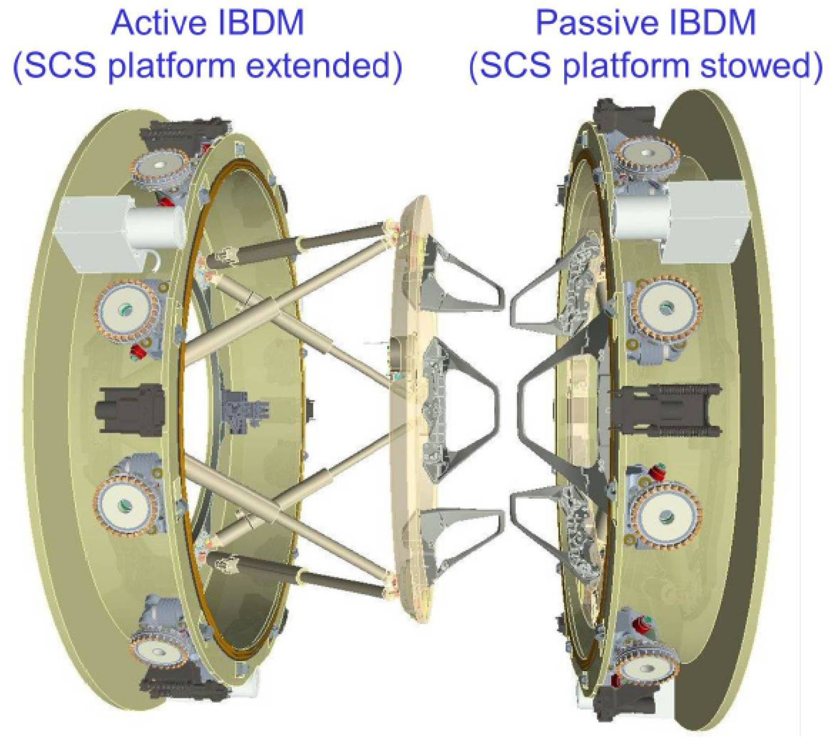
13]. However, the main difference to the lab-scale application is that BDM structures have high LPV dynamic properties. Since the leg’s dynamics depend on the experienced inertial load, each relative mass corresponds to a model with different dynamics. In other words, each model represents the dynamics of a particular leg in a particular pose when a certain force is exerted on the platform’s upper ring. Since every executable trajectory of the platform can be seen as a succession of different states, it is clear that the LEMA dynamics change constantly during spacecraft docking. How they become active during the contact process is briefly described as follows. During docking, the mechanism consists of an active and a passive module, as illustrated in
Figure 1, which can be viewed as two sub-systems with an interaction when in contact.
The ring-shaped interfaces of the active module can be moved with 6DOF by means of six telescopic extensible legs. The length of the legs is controlled for each leg individually by a brushless DC motor, based on the force signals measured by the load cells. Considering the platform’s 6DOF, the net power the legs have to deliver in order to move the spacecraft in a certain direction might differ, depending on the pose of the platform. When the actuator is oriented in the direction in which the platform has to be accelerated, the legs will experience low-load behavior, which is less demanding in terms of actuator effort. The variations in the load are referred to as the reflected mass. From an LPV perspective, this 6DOF platform has to be controlled with respect to a varying-load system conditions.
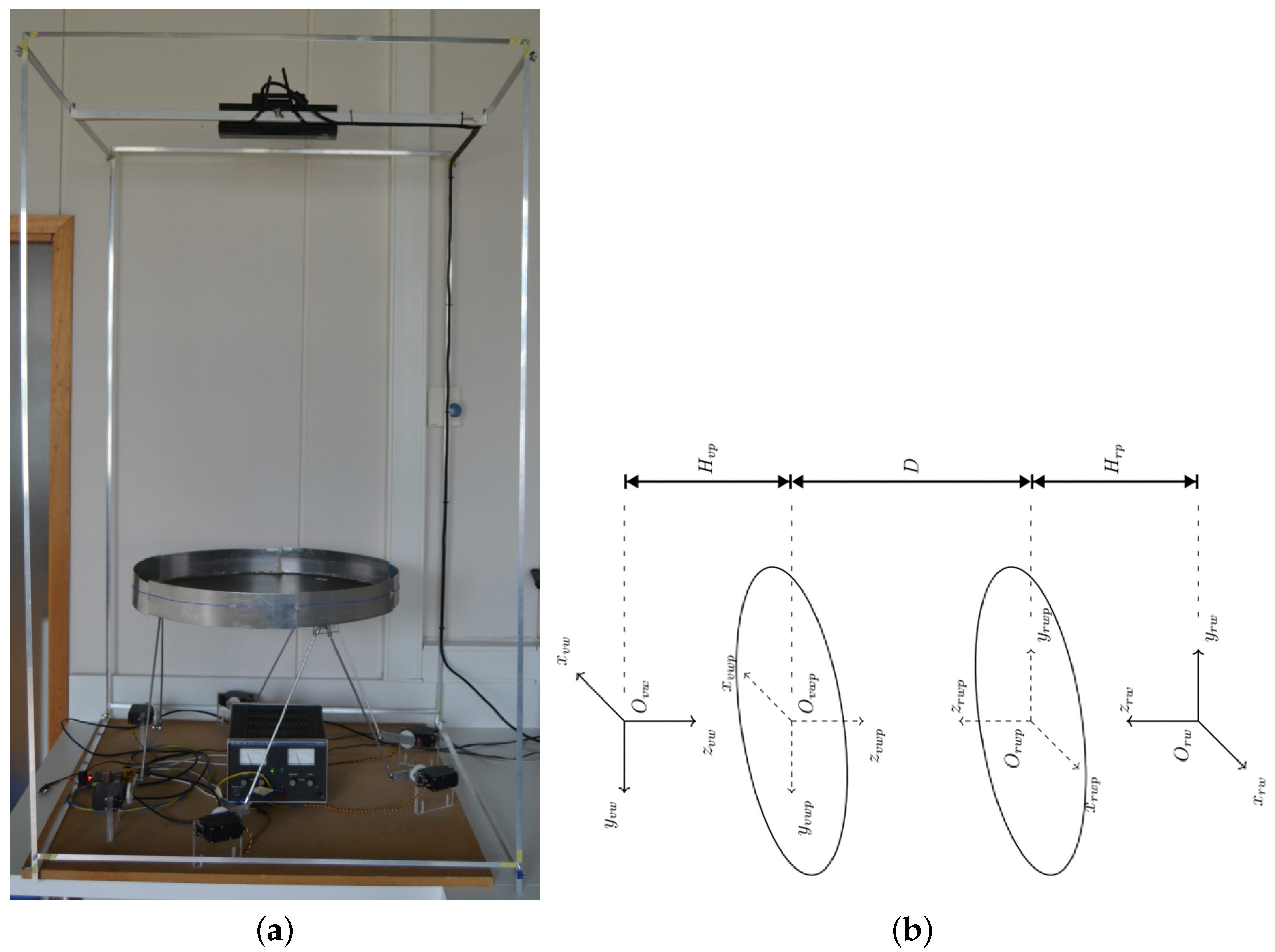
The real picture of the platform is depicted in
Figure 2a, while the coordinate system of the virtual and real platform is illustrated in
Figure 2b. In this figure, the
is the origin of the virtual world, the
is the central coordinate of the virtual platform and
and
represent the coordinates of the real world and of the real platform, respectively.
cm represents the height of the platform,
cm is the distance between the real ad the virtual platform, and the diameter of the platform plate is 70 cm. The real 6DOF platform from
Figure 2a represents the first part of the co-simulation setup system and is considered to be the active module of the BMD setup. It uses the position control of each leg (
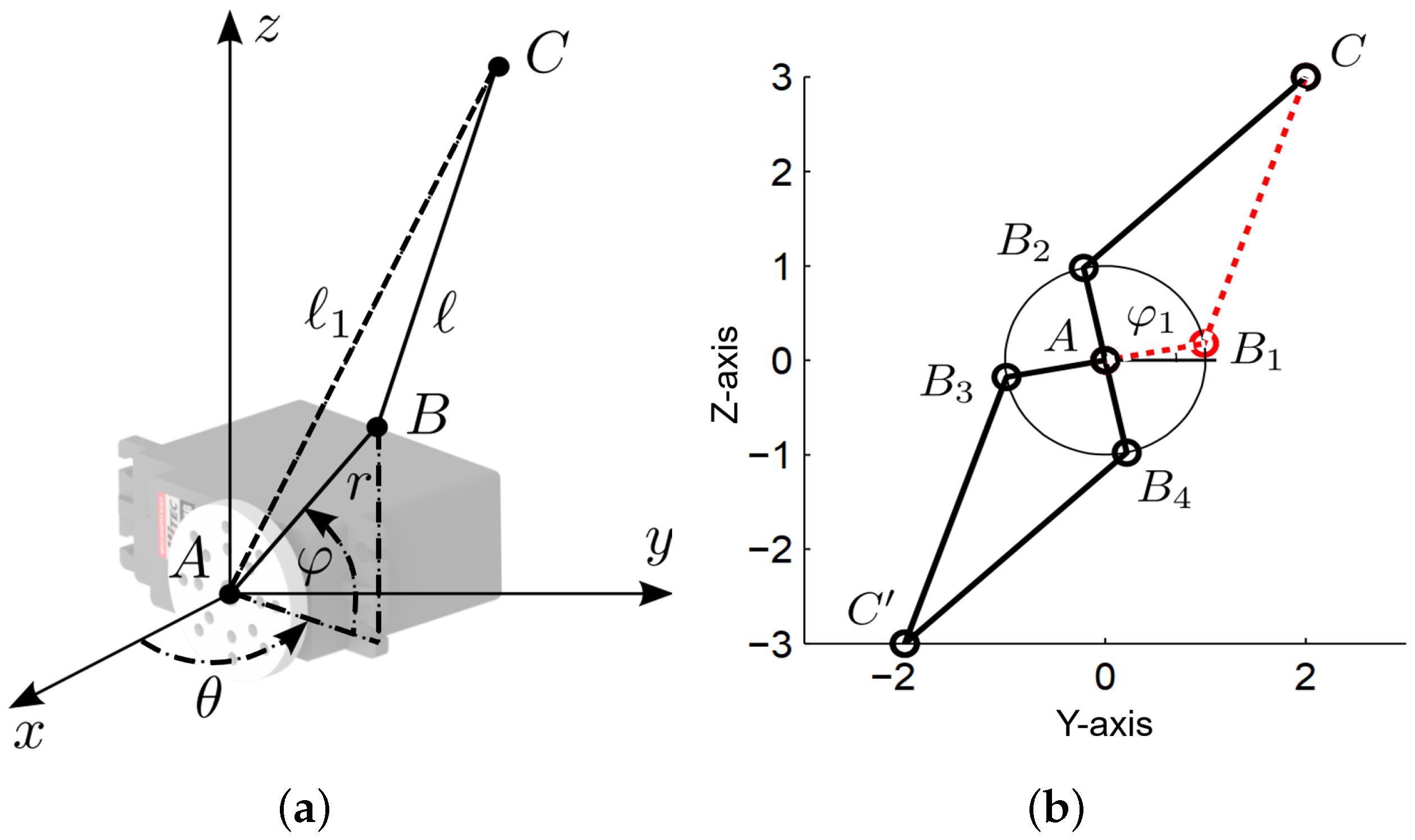
Figure 3a) to achieve global positioning and determine the angle of the platform.
Given that the position of the platform is known, the position of each connection
is also known (as specified by the controller). The position of the servo
and its orientation
are determined by the motion platform construction. The connection of the servo lever and the vertical rod is indicated as
. Let
r be the length of the servo arm (
) while
is the shaft that connects the servo arm with the platform in the point
C and has the length
ℓ. The absolute distance between point
A and
C is denoted by
. The inverse kinematic model is described as
where
The inverse kinematic model from (
1) has four solutions:
which are illustrated in
Figure 3b. Due to the employed mathematical method, a second point
is found; thus, solutions
and
(for points
and
) are discarded. Solution
and
(for points
and
) brings the connection
C to its desired position. As the servo position is restricted between
, solution
(point
) is selected as the unique feasible solution. The closed loop control uses classical visual feedback control based on camera vision information, as described in [
14].
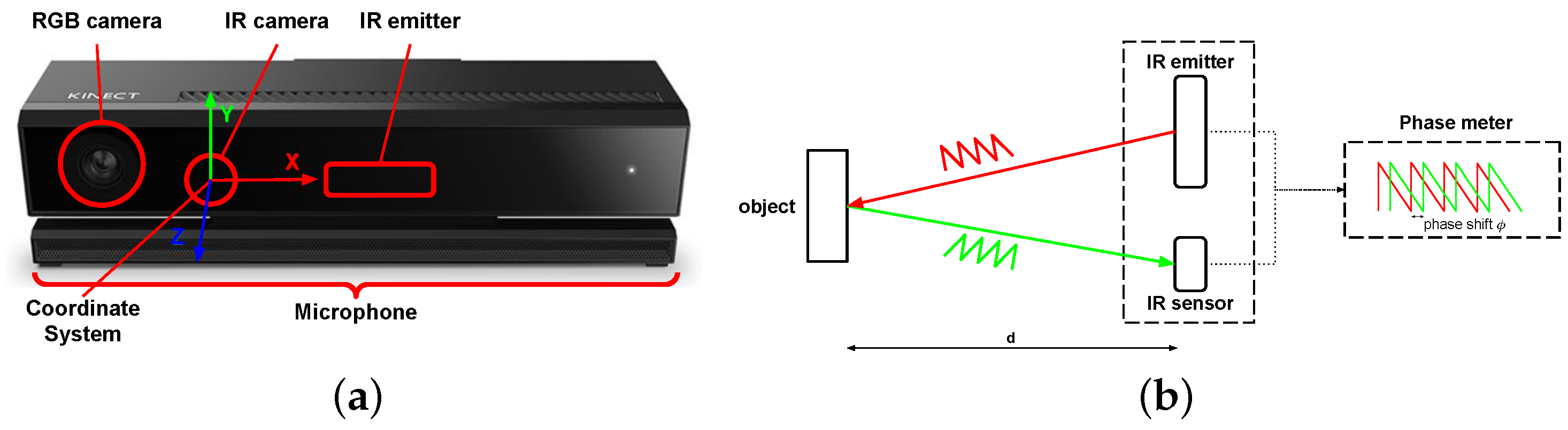
There are many possibilities for mapping a 3D environment, ranging from very expensive and accurate technologies to low-cost devices which are available for consumers. The Microsoft Kinect is a perfect example of such a low-cost sensor, and this has had a huge impact on recent research in computer vision as well as in robotics. Here, a Kinect v2 sensor is used as it was available in the laboratory. The Kinect v2 sensor holds two cameras (a RGB and an infrared (IR) camera), an IR emitter and a microphone bar, as shown in
Figure 4a. The Kinect software maps the depth data to the coordinate system, as shown in
Figure 4a, with its origin located at the center of the IR sensor. Note that this is a right-handed coordinate system with the orientation of the y-axis depending on the tilt of the camera and one unit representing one meter. Kinect v2 uses optical time-of-flight (ToF) technology in order to retrieve the depth data with the infrared (IR) camera. The basic principle of ToF is to measure the time difference between an emitted light ray and its collection after reflection from an object (
Figure 4b). The RGB-camera within the Kinect sensor has a resolution of 1920 × 1080 pixels with a field of view of 70.6 × 60 degrees, while the IR-camera resolution is 512 × 424 pixels and the field of view is 84.1 × 53.8 degrees. The operative measuring range of the Kinect sensor is between 0.5 and 4.5 m and the frame rate is 30 fps.
The intrinsic parameters of the depth camera of the Kinect, the focal length and the principal point, can be acquired using the Kinect For Windows SDK while the intrinsic parameters of the RGB camera can be acquired with the Camera Calibration Toolbox for MATLAB.
Next, the virtual model was constructed with a Siemens NX12.0 based on the existing 6DOF model of the platform [
10,
11,
12,
13]. Combining the NX12.0 Motion environment and the inverse kinematics calculations programmed in VisualBasic.Net, a simulation of the virtual world model was executed. Finally, a connection between the LabVIEW program and the NXOpen program was created using registry keys in the Windows Registry, as this allowed for the continuous monitoring of the keys without hindering access to the key from other processes.
In total, 13 VIs were generated to provide the necessary library for communication and the real-time operation of the real world platform and the virtual platform for mimicking a rendezvous. The LabVIEW platform provides the following features for the real-world 6DOF platform:
Communication with the 6DOF platform;
Kinematic calculations of the 6DOF platform;
A pinhole camera model;
Kinect data acquisition;
Visual data processing;
Calculations of the platform orientation;
The combination of the 6DOF platform communication and visual data.
NXOpen is a tool which is mainly used for computer-aided engineering (CAE)-purposes, and it allows the user to operate several functions of NX from a centralized location. In this case, NXOpen is used to allow the control of orientation of the platform in all its degrees of freedom, to set the duration of the simulation and to perform a static and dynamic analysis of the motion of the platform. Apart from taking the user input to control its position, it also allows the direct control of the servo angles and it permits the user to import data from the motion of the real-world platform in order to adapt to its orientation. It also starts the LabVIEW application when the simulation method is chosen.
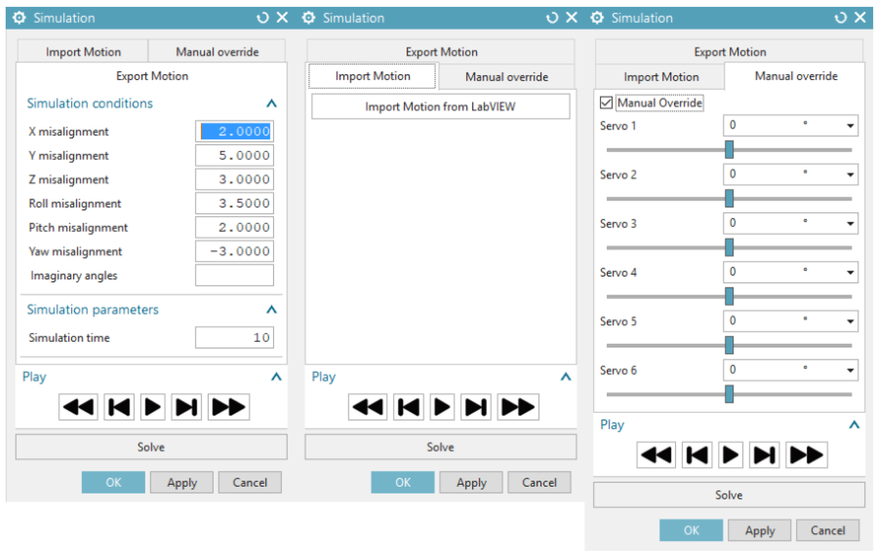
The code behind this graphical user interface (GUI) was written in VB.NET and consists of roughly five parts, with the result given in
Figure 5:
A part that is responsible for maintaining the GUI;
An object class to do the necessary calculations;
A method to export the values retrieved from the virtual sensors in the form of a .csv file;
A component to configure the motion functions of the servomotors;
A part that regulates the communication with LabVIEW through the use of registry keys.
As observed in
Figure 5, the user interface is divided inti three tabs:
Export motion is used to configure the attitude and position of the virtual platform. The values of servomotors are written in the text box besides the imaginary angles while filling in the values for the platform orientation—this makes it so that the values can still be adjusted before starting the solution. The simulation time defines the duration of the simulation;
Import motion: In this mode, a sequence of motion of the real-world-platform is imported and transformed to angles of the servomotors using the inverse kinematics, and then every point is plotted to form a motion-function. This motion function is then used as the driving function for the servo drivers;
Manual override is used to configure the angles of the individual servomotors. This function is primarily provided for testing purposes and has no influence on the real-world simulator.
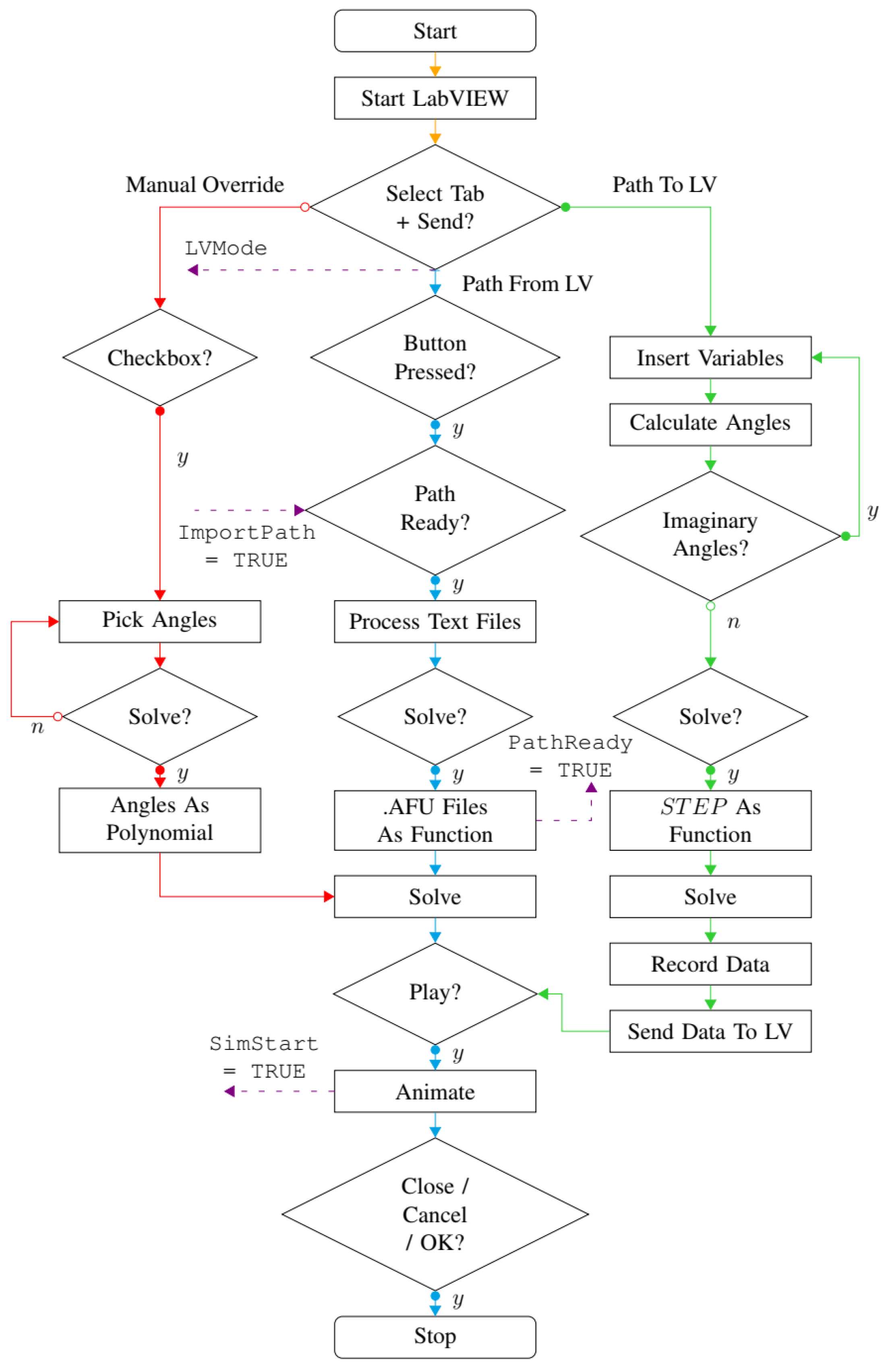
The overview of these three operating modes is illustrated in the flowchart in
Figure 6, where the red path represents the manual override mode, the blue path represents the import motion mode and the green path represents the export motion mode. The purple dash arrows represent the registry keys (SimStart, PathReady, LVMode, ImportPath) that are used to communicate with the LabVIEW application and ensure that the LabVIEW program does not skip steps the next time it executes. The overview of the working application (
Figure 6) shows the main steps in the communication and data processing parts necessary to allow the real-time co-simulation of the real world and virtual world platform setups as part of the docking mechanism.
2.1. Co-Simulation Procedure
The previous section gave a brief overview of both the LabVIEW and the VB.NET applications, while this section explains the cooperation between both applications. Both applications have the ability to influence each other, but only at specific points during the execution of the code, by reading and writing registry keys and by creating intermediary files to transfer large amounts of data. The communication via the registry keys is simply used as a confirmation and allows one application to know which part of the code the other application is executing. It can be said that the communication between LabVIEW and the VB.NET-application is a two-way communication process, but it is however not a simultaneous or continuous type of communication. Larger amounts of data are transferred between applications using both .csv-files and .txt-files, which results in another type of indirect communication. The motion sequence is recorded by six virtual sensors that are positioned at the center of the upper surface of the virtual platform. These sensors measure the displacement in three directions as well as the angular displacement around three axes. NX outputs the measurement data of the sensors as a binary file. These data are used as an input by LabVIEW to match the motion sequence of the real-world platform to that of the virtual platform. Because the data of the virtual sensors are used as a function of the virtual world coordinate system, this data have to be transformed to the real world-platform coordinate system using the principle illustrated in
Figure 4b. The real-world-platform motion-sequence is recorded by the Kinect sensor, which returns the platform orientation data. The data consist of three markers on the plate, which are detected by the visual sensor and are further used to calculate the platform position and attitude. The initial locations for each of these points is known, thus enabling us to calculate the transformation matrix between the initial location and the current location.
This co-simulation consists of two types of simulations:
The real-world simulation is in itself a real-time simulator: values that are changed on the front panel of the LabVIEW-app have an immediate effect on the orientation of the real-world platform;
The virtual-world simulation, however, is a slower-than-real-time-simulation because this application solves the entirety of the sequence at once before starting the animation.
The program mode that most closely resembles a synchronous simulation is the auto-mode. It records small motion-sequences with a step duration of approximately one 60th of a second, sends them to the virtual-world simulator and animates the simulation.
2.2. Simplified Model
The variation in the reflected mass for a single LEMA has been generated from real-life simulators and the data analyzed thoroughly in collaboration with QINETIC Space Kruibeke, Belgium (a confidentiality agreement is in place). To illustrate the high LPV degree in this berthing and docking mechanism system, we introduce a linear model approximation for the extreme cases. Since the leg positions must be controlled, these models capturing the leg dynamics can be approximated in the form indicated bellow:
where
K is the gain,
is a real zero,
denotes the complex comprised of
,
real poles and
denotes the complex comprised of
. This form of the transfer function has LPV parameter dynamics; i.e., changes in the
and
values. In order to illustrate the variability of the system, two extreme cases have been considered. The assumed linear model for case 1 is
The other extreme (case 2) of LPV dynamics is expressed by the system transfer function:
In this form of the models, the variations in pole/zero locations are clearly visible.
3. Adaptive Control
Originally, the controller used for this level was a single PI (proportional–integral) controller with feedforward action. An integer PI-cascaded controller has been outperformed in terms of robustness for maintaining closed loop specifications by a fractional order PI controller while being validated on the real-life simulator for European Space Agency at QINETIQ nva Antwerp, Belgium [
16]. A robust fractional order PI controller has been proposed and simulated in [
6]. Here, we use the adaptive robust fractional order PI (FOPI) control design described in [
5]. It has already been shown that fractional order control is a good candidate for the robust control of DC motor components [
17,
18,
19].
The FOPI described hereafter has the form:
where
and
are the proportional and integral gains and
the fractional order of integration. Note that the traditional PI controller is obtained for the special case when
. The fractional order PI controller in (
7) is thus a generalization of the integer order PI controller. The advantages of the fractional order PI controller stem from the extra tuning parameter
, which can be used to enhance the robustness of the controller. Since there are three tuning parameters in the fractional order PI controller, three performance specifications are used. These three performance criteria lead to the typical tuning rules for fractional order controllers. and they are based on the relationship between time-domain performance specifications and corresponding frequency domain specifications. We enumerate here the most commonly used specifications:
Gain cross over frequency , which is related to the settling time of the closed loop system—large values will yield smaller settling times at the cost of higher control efforts;
Phase margin (PM), which is stability related and an indicator of the closed loop overshoot percentage—usual values are within the
interval [
20];
The iso-damping property, which is a condition ensuring robustness to gain changes such that overshoot remains constant within a certain gain variation range.
To ensure a constant overshoot, a constant phase margin needs to be maintained around the desired gain crossover frequency, which ultimately implies that the phase of the open-loop system must be kept constant around the specified gain cross-over frequency. In other words, the derivative of the phase with respect to frequency around the gain cross over frequency must be (almost) null. The three performance specifications mentioned above are mathematically expressed as
where
stands for the open loop transfer function and
is the system to be controlled. Equations (
8)–(10) require the magnitude, phase and derivative of the phase for both the FOPI controller and
. The modulus and phase of the FOPI controller are given by
To determine analytically the derivative of the phase of the FOPI controller, the phase equation in (
11) is used, resulting in
Equations (
8)–(10) also use the magnitude, phase and derivative of the phase of
. The values for the modulus, phase and phase slope of the process should be known a priori at the gain cross over frequency
. These can be obtained analytically based on a model of
. Assuming a process model is given by Equation (
5), the magnitude, phase and derivative of the phase of
are computed as
To mimic a space rendezvous, the relative mass on each leg of the 6DOF platform can be varied at times during the simulation. In practice, the relative mass can be estimated continuously from the measured position and velocity of the platform. However, a continuous adaptation of controller parameters is not necessary and significantly increases the computational burden of the deployed system operation. Instead, using the standard performance index, a tolerance interval of is introduced in the overshoot () and settling time () values.
The relations in (
13) are easily computed online from previous samples’ reflected mass estimation. However, an additional condition of the violation of the tolerance interval is implemented to prevent the sluggish and unnecessary adaptation of controller parameters and consequently discretization and deployment on real-life emulator. The latter steps are performed solely when the threshold of tolerance interval is exceeded. Then, replacing (
11) and (
12) in (
8)–(10) leads to
With respect to the digital implementation of this controller, two more parameters are practically relevant: the degree of approximation and the user-specified
-range in which the desired behavior should be obtained, and tuning rules are given in [
21] (includes the Matlab function code provided in the paper).
4. Results and Discussion
The controller parameter solution for the isodamping property is achieved fora gain crossover frequency
of 150 rad/s and phase margin (PM) of
. The assumed linear model is (
5) and the resulting controller is
The parameters of the FOPI controller in (
15) were obtained by solving the set of nonlinear equations in (
14). First of all, the
parameter was estimated as a function of the fractional order
, using the phase margin and the iso-damping, according to the second and third equations in (
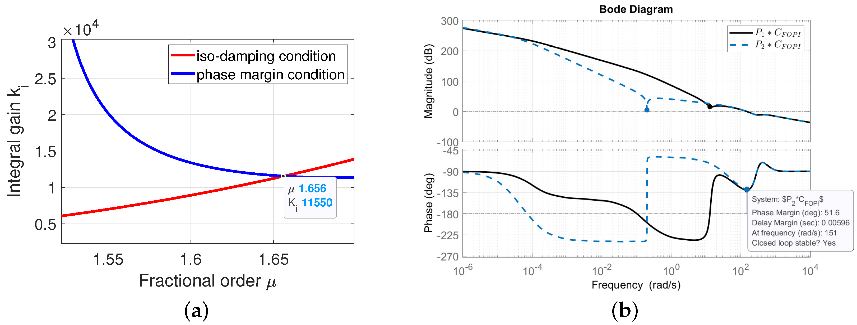
7). The two functions were then plotted as indicated in
Figure 7a. The intersection of the two functions gives the two control parameters that ensure both a certain phase margin and the iso-damping property. According to
Figure 7a, the intersection point yields
and
. Once these two parameters are computed, the proportional gain is estimated from the magnitude from the (first) equation in (
14) as
.
Figure 7b presents the Bode diagram for the controller and the two systems denoting two extreme cases (
and
) of LPV values (i.e., a variation of 250% in the reflected mass value in the 6DOF platform simulator).
The discretization scheme proposed in [
21] has been employed to obtain a discretized version of pole–zero pairs. This scheme is particularly efficient at delivering stable, low-order approximations of the non-rational function of the FOPI into a proper filter form, and for our study case, it delivers a fifth order rational transfer function.
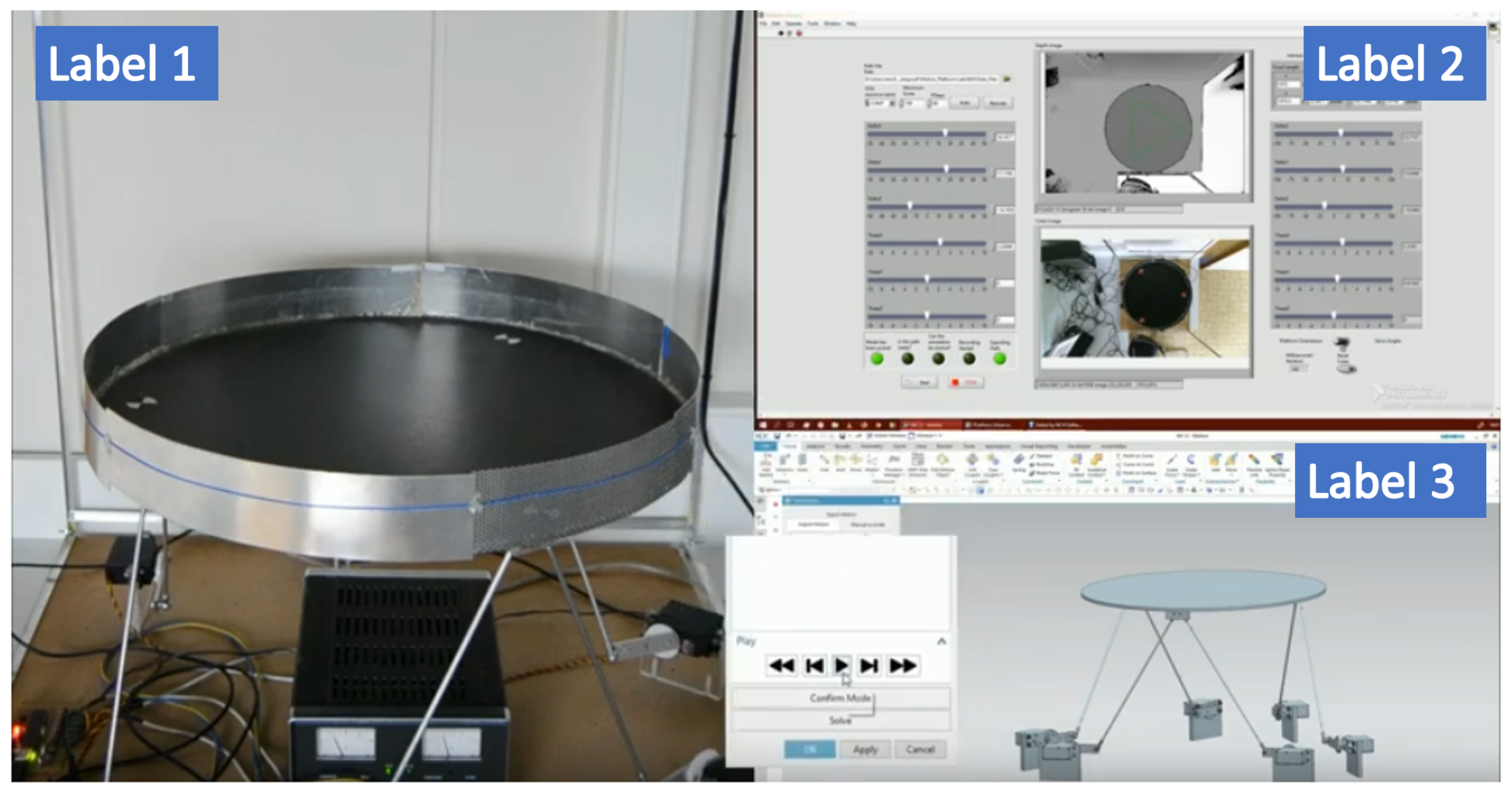
An example of a co-simulation interface and real-time tracking between the 6DOF platform and virtual model is illustrated in
Figure 8. In this figure, the real world platform can be observed, including the active part of the BDM system (label 1), the front panel of the LabVIEW application (label 2) and the 3D model of the simulated platform (label 3).
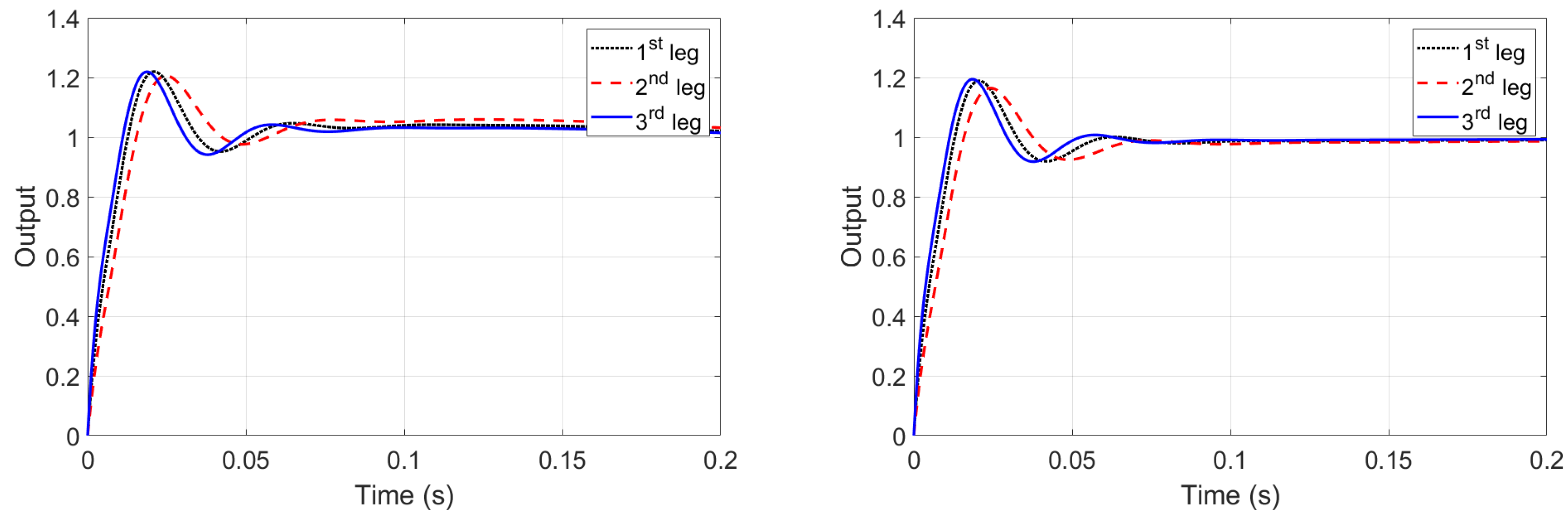
The adaptive controller maintains the same specifications in closed loop performance for the two variations in the reflected mass parameters, with the step response for three platform legs (the other are similar) given in
Figure 9. It can be observed that the controller maintains performance despite the great variability in system parameters mimicking the reflected mass for one leg with or without contact at docking.


