Article

Multi-Scale Safety Helmet Detection Based on SAS-YOLOv3-Tiny

College of Mathematics and Computer Science, Zhejiang Normal University, Jinhua 321004, China
*
Author to whom correspondence should be addressed.
Appl. Sci. 2021, 11(8), 3652; https://doi.org/10.3390/app11083652
Submission received: 23 March 2021 / Revised: 10 April 2021 / Accepted: 15 April 2021 / Published: 19 April 2021
(This article belongs to the Special Issue Computer Vision & Intelligent Transportation Systems)

Abstract

:
In the practical application scenarios of safety helmet detection, the lightweight algorithm You Only Look Once (YOLO) v3-tiny is easy to be deployed in embedded devices because its number of parameters is small. However, its detection accuracy is relatively low, which is why it is not suitable for detecting multi-scale safety helmets. The safety helmet detection algorithm (named SAS-YOLOv3-tiny) is proposed in this paper to balance detection accuracy and model complexity. A light Sandglass-Residual (SR) module based on depthwise separable convolution and channel attention mechanism is constructed to replace the original convolution layer, and the convolution layer of stride two is used to replace the max-pooling layer for obtaining more informative features and promoting detection performance while reducing the number of parameters and computation. Instead of two-scale feature prediction, three-scale feature prediction is used here to improve the detection effect about small objects further. In addition, an improved spatial pyramid pooling (SPP) module is added to the feature extraction network to extract local and global features with rich semantic information. Complete-Intersection over Union (CIoU) loss is also introduced in this paper to improve the loss function for promoting positioning accuracy. The results on the self-built helmet dataset show that the improved algorithm is superior to the original algorithm. Compared with the original YOLOv3-tiny, the SAS-YOLOv3-tiny has significantly improved all metrics (including Precision (P), Recall (R), Mean Average Precision (mAP), F1) at the expense of only a minor speed while keeping fewer parameters and amounts of calculation. Meanwhile, the SAS-YOLOv3-tiny algorithm shows advantages in accuracy compared with lightweight object detection algorithms, and its speed is faster than the heavyweight model.

1. Introduction

Driving a motorcycle or an electric two-wheeler without a safety helmet will cause a high mortality rate. However, many cyclists still have fluke psychology, so wearing safety helmets must rely on traffic policies’ way of compulsory supervision to attract people’s attention. At present, there are two main ways for traffic management departments to supervise whether riders wear helmets. In general, traffic policies check traffic surveillance videos manually. Another way is that traffic policies manage drivers and passengers on the road. These methods need a lot of human and material resources and cause the phenomenon of missing detection. Whether or not people who ride motorcycles and two-wheelers wear safety helmets to improve safety is crucial for intelligent traffic management, which has a significant research value. With the development of artificial intelligence, intelligent systems based on automatic image detection have been intensely studied and applied in different fields.
The task of object detection is to locate and classify objects in a given image. The uncertainty of object type and number, the diversity of object scale and the external environment’s interference will bring different degrees of influence to the task. Object detection algorithms based on convolutional neural networks are mainly divided into two categories: anchor-based and anchor-free. There are two types of anchor-based algorithm: two-stage algorithms represented by the Region-based Convolutional Neural Network(R-CNN) series and one-stage algorithms represented by the Single-shot multi-box Detector (SSD) series and the YOLO series. R-CNN [1] is a pioneering two-stage object detection algorithm proposed by Girshick et al., He et al. proposed SPP-Net [2] to accelerate R-CNN and learn more different features. Girshick et al. proposed Fast R-CNN [3], which used the Region of Interest (ROI) pooling layer to extract regional features. Object classification and bounding box regression can be optimized end-to-end without requiring additional cache space while it had better detection accuracy and faster reasoning speed than R-CNN and SPP-Net. Even though model learning has improved, the generation of the proposal still relied on traditional methods. Faster R-CNN [4] relied on a new proposal generator methods-Region Proposal Network (RPN), which can be learned by a supervised learning approach. Dai et al. proposed a Fully Convolution Network-based region (R-FCN) [5] to share the computational cost of region classification steps, compared with Faster RCNN, it achieves competitive results. In addition, a single deep feature map is used for final prediction in Faster R-CNN, which makes it difficult to detect objects of different scales, especially for small objects. Facing the problem, Lin et al. took advantage of different features and proposed Feature Pyramid Networks (FPN) [6], which combined deep features with shallow features. In order to make the whole detection process more flexible, He et al. proposed Mask R-CNN [7], which predicted bounding box and mask in parallel and reported the latest results. The two-stage algorithms above always divide the detection into two steps: proposal generation and proposal regression. The one-stage detection algorithms do not generate proposals. They categorize and locate each region of interest directly. Sermanet et al. proposed the one-stage detection algorithm OverFeat [8], which has a significant speed advantage. Redmon et al. developed a real-time detection algorithm called YOLO [9], and its entire framework is a single network, which omits the proposal generation step and can be optimized end-to-end. In 2016, SSD [10] was proposed to solve the limitations of YOLO. In the one-stage algorithm, the imbalance between foreground and background is a serious problem because there is no proposal generation to filter out easily generated negative samples, Lin et al. proposed RetinaNet [11] to solve the class imbalance problem in a more flexible way. Redmon et al. proposed an improved version of YOLO, YOLOv2 [12], which significantly improved the detection performance and maintained the real-time reasoning speed. Later, Redmon et al. proposed YOLOv3 [13], which used the Darknet-53 network structure and the idea of the residual network for reference. In addition, the idea of FPN was used to carry out multi-scale feature detection. The above improvements made YOLOv3 three times faster than SSD, while its accuracy is the same as SSD. Compared with the anchor-based algorithm, the anchor-free algorithms do not depend on the pre-defined anchors and avoid the complicated calculations related to the anchors. The earliest anchor-free methods are the Unifying Landmark Localization with End to End Object Detection (Densebox) [14] and YOLO [9]. The following anchor-free methods [15,16,17] are detection methods based on keypoints, and compared with YOLO and Densebox, the detection effect of these three methods is significantly improved. Finally, three methods [18,19,20] belong to the intensive prediction method, and they all obtain the desired result by directly predicting the rectangular box without using the anchor. In recent years, more and more object detection algorithms are applied in the security field. Haikuan Wang et al. put forward a real-time safety helmet wearing detection approach (named CSYOLOv3) [21], it achieved the mAP value of 67.05%, and its FPS reached above 25, so the mAP value was low and the speed was slow. Yang Li et al. proposed a deep learning-based safety helmet detection in engineering management based on convolutional neural networks [22], which would have a deficient performance when the images are not very clear, such as the safety helmets being too small and obscure. In addition, the above works only divide the categories of objects into two categories: Wear and Nowear, but the types of objects on the head are not distinguished. It is necessary to distinguish between different types of objects because ordinary hats are not safe, and different kinds of helmets have different protective effects on the head.
Experimental studies have found that the general object detection algorithms can be applied to the detection task of the safety helmet. However, under complex scenarios, the small-scale object is sheltered and it is dense. The remote small-scale safety helmets and hats with low resolution and blurry pixels have less characteristic information, which leads to the phenomenon of missed detection. In addition, it is challenging to balance the accuracy and complexity in general object detection algorithms, and the imbalance between the two makes it difficult to deploy on mobile devices. Even though YOLOv3 is a widely used object detection algorithm with good recognition speed and detection accuracy by combining several methods such as residual network, feature pyramid and multi-feature fusion network, it has lots of parameters and amount of computation and generates a large model. Hence, it is challenging that the model is transplanted to embedded applications when computing power and storage space are limited. YOLOv3-tiny based on YOLOv3 is a lightweight object detection network applying an embedded platform, but its detection accuracy is low. In this paper, SAS-YOLOv3-tiny is proposed to balance the detection accuracy and speed for a set of self-built helmet datasets. Aiming to promote detection effect while reducing the number of parameters and calculation amount, the Sandglass-Residual module based on depthwise separable convolution and channel attention mechanism is constructed to replace the traditional convolution layer while the convolution layer of stride two is utilized into the backbone to replace the max-pooling layer, which can extract informative and high-dimensional features. The three-scale feature prediction method is introduced into the network structure of SAS-YOLOv3-tiny to improve the two-scale feature prediction for obtaining accurate location information of small objects further. The improved spatial pyramid pooling module is applied to enhance the feature extraction further. CIoU is used to promote the loss function to improve location accuracy. Our algorithm achieved the mAP value of 81.6% on the validation set and the mAP value of 80.3% on the test set with the average detection time of 3.2 ms on each image under an actual traffic environment.
The rest of the paper is organized as follows. Section 2 will explain the principles of the original algorithm YOLOv3-tiny. Section 3 will describe the innovation points of the improved algorithm (SAS-YOLOv3-tiny) in detail. Section 4 will show some experimental results and analyze them. Finally, in Section 5, this paper will be summarized and some future works will be proposed.

2. The Principles of YOLOv3-Tiny

In this section, we will mainly introduce the principles of YOLOv3-tiny. In Section 2.1, the network architecture of YOLOv3-tiny will be defined in detail. In Section 2.2, the principle of bounding box prediction will be explained. The above principles lay a solid foundation for the improved algorithm in Section 3.

2.1. Network Architecture of YOLOv3-Tiny

YOLOv3-tiny is an improved version of YOLOv3, which has changed the YOLOv3’s backbone network (named Darknet53) to seven convolution layers with kernel size of 3 × 3 and six max-pooling layers with stride 2. The idea of FPN is adopted to integrate feature map with low resolution and feature map with high resolution. YOLOv3-tiny utilized last two downsampled feature maps with size of 28 × 28 × 256 and 14 × 14 × 1024 to predict the objects. The reason is that the feature map with size of 14 × 14 × 1024 contains abstract and high-level semantic information while the feature map with size of 28 × 28 × 256 carrying more detailed and lower-level location information, which can obtain feature map containing both semantic and positional information. Specifically, the input image with size of 448 × 448 × 3 is processed through the backbone network and a convolution operation, producing the resultant feature map with size of 14 × 14 × 1024 . One part of the processed results is processed through the convolutions and used to output predictions in terms of the current feature map, and the other part is processed through a convolution layer and an up-sampling operations, and then is fused with the corresponding upper feature map with size of 28 × 28 × 256 . The above operations can obtain the feature map with size of 28 × 28 × 384 , which is processed by the convolutions, and then used for prediction. At scale y1, the feature map downsampled by 32 × is utilized to detect larger objects. At scale y2, the feature map downsampled by 16 × is responsible for detecting smaller objects. YOLOv3-tiny network’s structure is demonstrated in Figure 1.

2.2. Bounding Box Prediction

YOLOv3 continued to employ K-means clustering of YOLOv2 to determine the prior boxes, which drew on the anchor box mechanism of RPN in Faster R-CNN. K-means clustering algorithm in YOLOv3-tiny obtained K prior boxes on the Common Objects in Context (COCO) dataset according to the annotated ground truth boxes, which could improve the detection accuracy and speed. Joseph Redmon et al. modified the clustering distance in the k-means algorithm [12]. As shown in Formula (1), it is defined by IOU. The larger the IOU is, the closer distance of the two bounding boxes is.
d ( b o x , c e n t r o i d ) = 1 I O U ( b o x , c e n t r o i d )
In Formula (1), d ( b o x , c e n t r o i d ) represents the clustering distance, c e n t r o i d represents the box that is selected as the center of mass by the algorithm, b o x represents the other bounding boxes and I O U represents the ratio of the intersecting area of the two boxes to the combined area. Even though too many prior boxes can guarantee the detection effects, it greatly affects the efficiency of the algorithm. YOLOv3-tiny used six prior boxes. The corresponding relationship between feature maps and prior boxes is as follows. Feature maps of size 14, 28 correspond [(81,82); (135,169); (344,319)], [(10,14); (23,27); (37,58)], respectively. Generally, large feature maps usually have small receptive fields, which are very sensitive to small-scale objects, and thus, they will select small prior boxes. On the contrary, small feature maps always have large receptive fields, which are suitable for detecting large objects, and thus, they select large prior boxes.
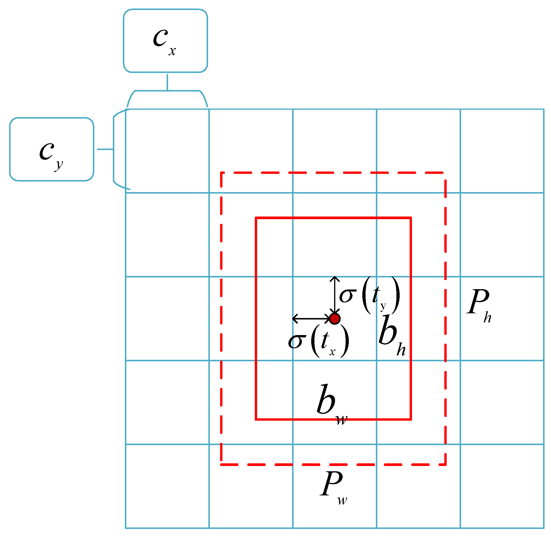
The final predicted bounding box coordinates of the YOLOv3-tiny network can be obtained by Formulas (2) and (3), and the final bounding box prediction schematic is shown in Figure 2. The confidence is divided into two parts: one is the probability of the existence of the object, showed by P r ( o b j e c t ) (if the object exists, P r ( o b j e c t ) = 1 , otherwise it is 0), while the other is the accuracy of the predicted bounding box, which is shown in Formula (4).
b x = σ ( t x ) + c x b y = σ ( t y ) + c y
b w = p w e t w b h = p h e t h
C c o n f = P r ( c l a s s i | o b j e c t ) × P r ( o b j e c t ) × I O U p r e d t r u t h = P r ( c l a s s ) × I O U p r e d t r u t h
In Formulas (2) and (3), b x and b y are the coordinates of the center point of the modified bounding box; b w and b h represent the width and height of the modified bounding box, respectively; t x and t y represent the offset between the object center point and the upper-left corner of the grid; t w and t h represent the offset of the width and height of the predicted bounding box, respectively; c x and c y represent the offset of the grid relative to the upper-left corner. p w and p h are the width and height of the prior box, respectively. The sigmoid function is used to control the range of value within (0, 1) and control the offset of the object center within the corresponding grid cell to ensure that it is not out of bounds. In Formula (4), C c o n f represents the confidence score of a specific category for each box; P r ( c l a s s i | o b j e c t ) represents the probability of predicting C conditional class in each grid cell (I = 1, 2,…, C); P r ( o b j e c t ) × I O U p r e d t r u t h represents the confidence score; I O U p r e d t r u t h represents the intersection ratio of the ground truth box and the prediction box.

3. SAS-YOLOv3-Tiny Algorithm

The original YOLOv3 algorithm has a considerable computation cost and parameters, which are not suitable for deployment on mobile devices. Therefore, YOLOv3 does not satisfy the specific application domain, such as helmet detection. Even though YOLOv3-tiny can meet the practical needs in terms of computation amount and number of parameters, which is not as accurate as YOLOv3 due to model compression. To further reduce the number of parameters and the amount of calculation, the Sandglass-Residual module will be proposed in Section 3.1. Meanwhile, the channel attention mechanism will be fused into the Sandglass-Residual module to extract more valuable features. In Section 3.2, the improved SPP module will be introduced into the SAS-YOLOv3-tiny network architecture to obtain local and global features. In Section 3.3, we will show the overall network architecture of SAS-YOLOv3-tiny, which utilizes three-scale feature prediction to promote the small-scale objects’ detection performance. CIoU loss will be applied to the original loss function to improve position accuracy in Section 3.4.

3.1. Sandglass-Residual Module Based on Channel Attention Mechanism

The inverted residual module of MobileNetv2 [23] places the shortcut on the low-dimensional representations. Feature compression will cause some problems that optimization is complicated, and the gradient is easy to shake, affecting the convergence of the model. MobileNext [24] proposes a new sandglass bottleneck module to solve the inverted residual module problem, which puts the shortcut on the high-dimensional representations. The above operations can retain the advantages of high-speed convergence and training on the high-dimensional network and take advantage of the computational advantages of depthwise separable convolution. In general, the parameters and calculation amount of traditional convolution increase significantly with the increase of convolution layers. So the conventional convolution is replaced with depthwise separable convolution to reduce model complexity, which is transformed into two parts: depthwise convolution and point convolution. We assume that the size of input feature map is D F × D F × M , the size of output feature map is D F × D F × N and the size of standard convolution kernel is D K × D k × M . The computation amount of standard convolution is D K × D K × M × N × D F × D F . In the depthwise convolution operation, the size of convolution kernel is D k × D k × 1 and its number is M. In the point convolution operation, the size of convolution kernel is 1 × 1 × M and its number is N. so the computation amount of depthwise separable convolution is D K × D K × M × D F × D F + M × N × D F × D F . By comparing the computational amount of the two, the computational amount of depthwise separable convolution can be reduced to 1 / N + 1 / D K 2 of the standard convolution.
In our work, the Sandglass-Residual module based on the lightweight idea is constructed in the feature extraction process, ensuring that more information is passed from the bottom to the top and gradient propagation is facilitated. The Specific operations are as follows. In the high-dimensional space, two depthwise convolutions with kernel size of 3 × 3 are performed, which can encode more spatial information. The point convolution with kernel size of 1 × 1 is utilized to reduce and increase channels’ dimensions and encode information between channels. The first depthwise convolution and the last point convolution use nonlinear activation functions. In contrast, the first point convolution and the final depthwise convolution directly perform linear output to avoid information loss. The parameters of the Sandglass-Residual module are shown in Table 1.
The YOLOv3-tiny algorithm is applied to a real-world scenario dataset, objects in the image are treated equally. If the weight is assigned to the features of the object area, the weighted feature maps will be conducive to detecting far-distance and small-scale safety helmets, which can improve detection accuracy without introducing too many parameters. The Squeeze-Excitation (SE) channel attention module in SENet [25] gives different weights to different channels in the feature map of the convolutional neural network, making the network pay more attention to the channels with higher weights. Thus, it can enhance the learning ability of the network, and its specific operations are as follows. The feature map with size of H × W × C is compressed into a vector that its size is 1 × 1 × C by compression operation (i.e., global average pooling operation). Then the weights of different channels are obtained by excitation operation (i.e., two fully connection operations), and finally, the feature weighting operation is carried out on the obtained feature maps. After the above operations, the attention feature maps are produced. All channels of the feature maps generated by the above Sandglass-Residual module are treated equally, which makes some essential features be overlooked so that these obtained features are not conducive to detecting difficult-to-distinguish objects. Therefore, in this paper, the channel attention is introduced into the Sandglass-Residual module to extract informative features, adjusting the characteristic relationship between network models by squeeze and excitation operations. Its structure is shown in Figure 3. Compared with the original SR block, the Sandglass-Residual module based on the Squeeze-Excitation channel attention enhances the network’s nonlinear characteristics, which can improve the model generalization ability without changing the output dimension. The subsequent ablation experiments prove that the Sandglass-Residual module based on the Squeeze-Excitation channel attention is good for improving the detection performance.

3.2. Improved Spatial Pyramid Pooling Module

To obtain the context semantic information of different receptive fields and further improve the detection accuracy of the model, an improved spatial pyramid pooling (SPP) module is added into the improved backbone network. The traditional spatial pyramid pooling [2] is to solve the problem that the input of the fully connected layer must be a fixed eigenvector, which allows us to build a network that supports images of any size to input without cropping and scaling operations. The spatial pyramid pooling module in this paper integrates multi-scale local feature information with global feature information to obtain richer feature representations, which is shown in Figure 4.
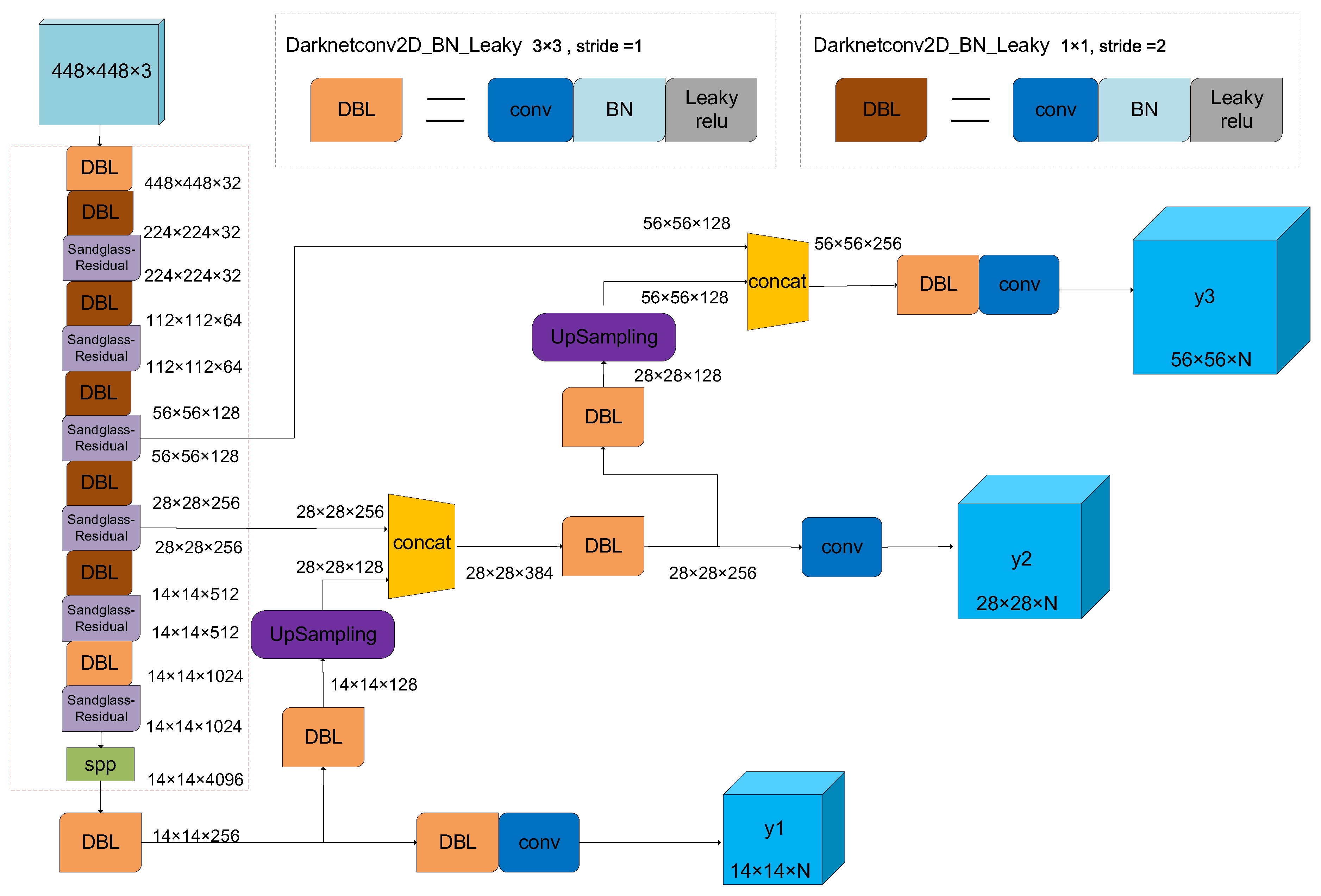
After going through the improved SPP module, the feature map’s size stays the same, realized by the pooling operation of stride one and the padding method. Specifically, the final feature map with size of 14 × 14 × 1024 extracted from the backbone network already contains rich semantic information. After that, three max-pooling operations are adopted to obtain three kinds of feature maps, which are concatenated with the input feature map with size of 14 × 14 × 1024 along the channel dimension to produce the feature map of size 14 × 14 × 4096 as the output. 5 × 5 , 9 × 9 , 13 × 13 are the size of the pooling kernel, while the stride is 1. The experiments show that the improved SPP module is added after the backbone network to extract rich features, improving the detection effect.

3.3. Network Architecture of SAS-YOLOv3-Tiny

To solve low detection accuracy and high missing rate of YOLOv3-tiny on small objects such as helmets, we have improved the original network. The network structure of SAS-YOLOv3-tiny is shown in Figure 5. The backbone network of SAS-YOLOv3-tiny is constructed by combining the previously made Sandglass-Residual module based on the Squeeze-Excitation channel attention and the improved SPP module based on spatial pyramid pooling. To be specific, in Figure 5, the dashed line part is the feature extraction part of the backbone network, in which five brown DBLs in the middle of the backbone network are the 1 × 1 convolution layer of stride 2 to replace the max-pooling layer to perform down-sampling operations and change the number of channels. The five Sandglass-Residual in the middle of the backbone are the Sandglass-Residual modules based on the Squeeze-Excitation channel attention to replace the standard convolution layer behind the max-pooling layer of the original backbone network. Furthermore, to make the network more robust, we add the improved SPP module at the end of the backbone network to fully extract local and global features.
Simultaneously, we improved the method of multi-scale feature fusion. Based on the original network’s two-scale feature prediction, a downsampled feature map with size of 56 × 56 × 128 is used to form the three-scale feature prediction to improve object detection accuracy further. In addition to being used as prediction, the feature map with size of 28 × 28 × 384 after a convolution operation continue to go through a convolution layer and an upsampled layer, and then is concatenated with the feature map with size of 56 × 56 × 128 to perform prediction. At scale y3, the feature map downsampled by 8 × is utilized to detect small objects, because it can get more detailed features and location information of small objects. In the improved algorithms, nine prior boxes instead of six prior boxes are utilized, and the corresponding relationship between feature maps and prior boxes is as follows. Feature maps of size 14, 28, 56 correspond [(373,326); (156,198); (116,90)], (59,119); (62,45); (30,61)], [(10,13); (16,30); (33,23)], respectively.

3.4. Improved Loss Function

Recently, in terms of bounding box regression, IOU loss optimizations have replaced previous regression loss optimizations (MSE loss, L1-Smooth loss, etc.). One of the most commonly used evaluation criteria for the performance of object detection algorithms is intersection over union (IOU), which is the ratio of the overlap area of the ground truth box and the prediction box to the total area of the two boxes, as shown in Formula (5). In Formula (5), A = ( x , y , w , h ) represents the prediction box and B = ( x g t , y g t , w g t , h g t ) represents the ground truth box.
I O U = | A B | | A B |
Even though IOU can reflect the detection effect of the prediction box and the ground truth box, it only works when the bounding boxes overlap and does not provide any adjustment gradient for the non-overlapped part. The concept of IOU is based on the ratio, so it is insensitive to the object scale. In this paper, in Formula (6), the traditional regression loss MSE is replaced with CIoU [26], whose detection effect is more conducive to the actual scene. It inherits the advantages of the Generalized Intersection Over Union (GIoU) [27] and Distance-IoU(DIoU) [28], which not only considers the distance and overlap ratio but also considers the scale and the aspect ratio between the prediction box and the ground truth box so that it can carry out the bounding box regression better. The complete definition of CIoU loss function is shown in Formula (7). Therefore, the loss function of SAS-YOLOv3-tiny is shown in Formula (6), which is divided into three parts: l o s s C I o U represents the regression loss, l o s s o b j represents the confidence loss and l o s s class represents the category loss, they are shown as shown in Formulas (7)–(9).
L O S S = l o s s C I o U + l o s s o b j + l o s s c l a s s
l o s s C I o U = 1 C I o U C I o U = I O U ρ 2 ( b , b g t ) c 2 α ν
l o s s o b j = i = 0 K × K j = 0 M I i j o b j [ C i log ( C i ) + ( 1 C i ) log ( 1 C i ) ] λ n o o b j i = 0 K × K j = 0 M I i j n o o b j [ C i log ( C i ) + ( 1 C i ) log ( 1 C i ) ]
l o s s c l a s s = i = 0 K × K I i j o b j c c l a s s e s [ p i ( c ) log ( p i ( c ) ) + ( 1 p i ( c ) ) log ( 1 p i ( c ) ) ]
In Formula (7), b and b g t represent the center points of the prediction box and the ground truth box, respectively. Meanwhile, ρ 2 ( b , b g t ) represents the Euclidean distance between two center points, c represents the diagonal distance of the smallest closure region that can contain both the prediction box and the ground truth box, α is the weight parameter and ν is used to measure the similarity of aspect ratios. In Formulas (8) and (9), K × K represents the size of the final feature map to be detected; I i j o b j is used to determine whether the j-th prior box in the i-th grid is responsible for the object. If it is responsible for the object, it has a value of 1. Otherwise, its value is 0. The weight coefficients λ c o o r d and λ n o o b j are set at 5 and 0.5, respectively, which are used to offset the imbalance between positive and negative samples.

4. Experiments and Results Analysis

In Section 4, some experiments and results analysis will be explained in detail. The basic information of safety helmet detection dataset and evaluation criteria of detection effect will be introduced in Section 4.1. Then, we will explain the experimental progress and do a result analysis in Section 4.2. There are four subsections in Section 4.2. In Section 4.2.1, we will describe the training setting. In Section 4.2.2, we will do ablation experiments to prove the effectiveness of each scheme. In Section 4.2.3, we will conduct the comparison of results with other state-of-the-art detection models. In Section 4.2.4, we will show the detection results of some samples under different detection models.

4.1. Dataset and Evaluation Criteria

4.1.1. Dataset

Dataset is crucial for deep learning-based object detection algorithms. In our work, a set of safety helmet datasets was made, which contained 7656 images and was obtained by searching on the Internet, taking photos with cameras and web crawlers, and the format was produced in VOC format. Labeling software (labelImg) was used to label the collected images. There were four categories of objects: helmet (wear a safety helmet for two-wheelers), cap (wear a non-protective hat), Nowear (wear nothing) and safety-cap (wear an industrial helmet). Additionally, the annotated image coordinate information was saved as an XML file. Next, the training set, the validation set and the test set were randomly divided, and the 8:1:1 ratio was adopted in our study, so there were 6063 training samples, 827 validation samples and 766 test samples. Specifically, the training set was used to train parameters of neural network. The validation set was used to test the effect of the current model after each epoch. The test set was used to test the model’s final generalization performance because it did not participate in the training process at all.

4.1.2. Evaluation Criteria

The quality of the detection effect usually needs a certain standard to evaluate, so the following evaluation criteria are introduced.
(1) The formulas of the Precision and Recall are shown in Formula (10), and the formula of F1 is shown in Formula (11). F1 is the harmonic mean of Precision and Recall. In Formula (10), True Positives (TP, IOU ≥ threshold) refers to the number of instances that are actually positive examples and are classified as positive examples by the classifier. False Positives (FP, IOU < threshold) refers to the number of instances that are actually negative examples but are classified as positive examples by the classifier. False Negatives (FN, undetected ground truth box) refers to the number of instances that are actually positive examples but are classified as negative examples by the classifier.
P p r e c i s i o n = T P T P + F P R r e c a l l = T P T P + F N
F 1 = 2 P R P + R
(2) The formulas of Average Precision (AP) and Mean Average Precision (mAP) are shown in Formula (12).
A P = 0 1 P ( R ) d R m A P = i = 1 N A P i N
In Formula (12), N represents the number of object categories. In general, the increase of the Recall is often accompanied by a decrease in Precision. To better balance the two, the P-R curve is introduced, and the area below it is the AP value of a specific category.

4.2. Experimental Progress and Result Analysis

4.2.1. Training Setting

This paper’s experimental platforms were Intel(R) Core (TM) I7-9700 CPU @3.00 GHz processor and NVIDIA GeForce RTX 2080Ti GPU. The programming language used for the algorithm in this paper was Python 3.8. The deep learning framework Pytorch 1.6.0 was used. The operating system used was Ubuntu18.04, and other dependent libraries were configured. Generally speaking, there were two training methods to train the model. One method was that random initial weights were used to train the model. The other is that pre-training weights were used to train the model. This paper used the first method to train the model to compare the different modification methods. In the experiment, the SAS-YOLOv3-tiny network was trained from scratch by using a self-built dataset. To ensure the fairness of the test, we retrained the YOLOv3-tiny, YOLO v3 and v4 [29] in the same experimental environment to obtain the corresponding detection model for experimental comparison results of the improved algorithm model on the validation set and the test set. Some experimental parameters were set as follows. In the experiment, the batch size was set to 4; 140 epochs were trained; the cosine learning rate strategy was used, which changed the learning rate from 0.01 to 0.0005; momentum was set to 0.937; weight decay was set to 0.000484. In addition, the multi-scale training strategy was adopted to improve the detection effect of the network for images of different input resolutions, and the cut size was selected at {320,352,384,416,448,480,512,544,576,608,640} for training in each iteration.

4.2.2. Ablation Experiments

In this section, to better understand the influence of each improved method on the detection effect, ablation learning is carried out on the self-built helmet validation set. First of all, we first presented each of our schemes in Table 2. Then, we compared different modification schemes based on YOLOv3-tiny in terms of indicators including P, R, F1, mAP, Weight, Total Parameters and average time of detecting a single image (detection time) in Table 3, and comprehensively analyze how each improvement point promote performance. Finally, we demonstrated the effectiveness of the improvement point by presenting a training curve for each scheme.
The different schemes are shown in Table 2. We used the yolov3-tiny algorithm as the baseline. Specifically, in the scheme SR, the Sandglass-Residual (SR) module was used to replace the original convolution layer, and the max-pooling layer was replaced with the convolution layer of stride two. In the scheme SR-3 scale (3 s), on the basis of the scheme SR, a three-scale prediction method was adopted. In the Scheme SR-3s-SPP, to further improve the detection effect, the improved SPP was utilized on the basis of the Scheme SR-3s. In addition, in the Scheme SR-3s-SPP-SE, the Squeeze-Excitation (SE) channel attention mechanism was integrated into the Sandglass-Residual module to extract more representative features on the basis of the Scheme SR-3s-SPP. In the Scheme SR-3s-SPP-SE-CIoU, we used CIoU loss on the basis of the Scheme SR-3s-SPP-SE. A combination of five improvements formed our final algorithm, in other words, the last Scheme SR-3s-SPP-SE-CIoU was our improved algorithm (named SAS-YOLO-v3-tiny).
The ablation results of different models on the validation set are shown in Table 3. From Table 3, we can see that the values of indicators including P, R, mAP, F1 are low in the original YOLOv3-tiny algorithm. Additionally, the indicators, including the weight size of the model and total parameters, still have room for improvement. Compared with the original algorithm, the improved YOLOv3-tiny based on the Sandglass-Residual module made the network more lightweight; this was because the Scheme SR based on depthwise separable convolution reduced the number of parameters and computation amount, reducing the size of weight files and the number of parameters by nearly half. In addition, owing to putting the shortcut on the high-dimensional representations, the SR module could extract rich feature, which could increase R by 4.6%, increase mAP by 4.5% and increase F1 by 1.4% while keeping the detection speed almost unchanged. The Scheme SR-3s changed two-scale feature prediction into three-scale feature prediction, which could incorporate shallow features with sufficient location information, making R, mAP, F1 increase by 1.7%, 2%, 0.9%, respectively. The introduction of the improved SPP module in the Scheme SR-3s-SPP could extract feature with different receptive fields, which can further improve P, R, F1 by 0.7%, 0.8%, 0.8%, respectively. Based on the Scheme SR-3s-SPP-SE, the channel attention mechanism was introduced into the Sandglass-Residual module, which could pay attention to useful feature, improving P, mAP and F1 by 2.0%, 1.1%, 1.0%, respectively. Further, CIoU loss was utilized in the final Scheme SR-3s-SPP-SE-CIoU to promote positioning accuracy, which could improve P by nearly 1%. Due to the combination of the above improved methods, compared with the original YOLOv3-tiny, SAS-YOLOv3-tiny had advantages on model performance and complexity. Specifically, it improved P by 2.5%, improved R by 6.9%, improves mAP by 7.9%, improved F1 by 4.5% over the original algorithm on the validation set and had a smaller number of parameters than the original algorithm at a sacrifice of only 0.8 ms.
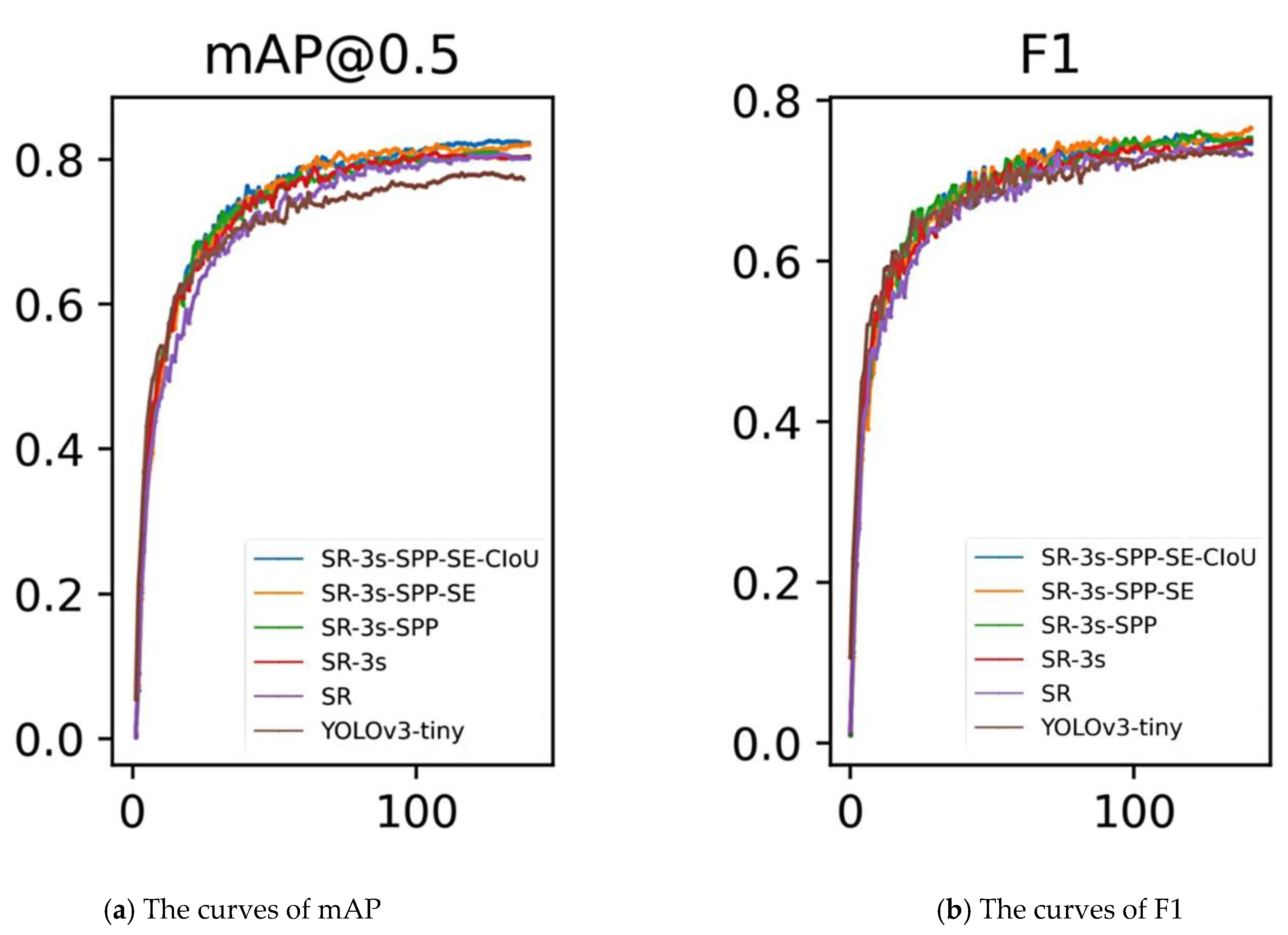
To further demonstrate the effectiveness of different schemes, we presented the curves in the training process for six groups of experiments. Two critical performance indicators are mAP and F1, the curves of F1 and mAP in the different models are shown in Figure 6a,b. The horizontal axis in the Figure 6a,b represents the training time, while the vertical axis represents the value of F1 and mAP, respectively. The YOLOv3-tiny represents the training curves of the original algorithm, in which the mAP value and F1 value are the lowest. The SR represents the training results of the Scheme SR, the main reason for the promotion of performance is utilization of the Sandglass-Residual module. The SR-3s represents the training process of the Scheme SR-3s, in which the Sandglass-Residual module and the three-scale feature prediction are applied simultaneously, promoting further enhancement in terms of the mAP and the F1. The SR-3s-SPP represents the training curves of the Scheme SR-3s-SPP, in which not only the Sandglass-Residual module and the three-scale feature prediction are adopted, but also the SPP module is employed. The application of the SPP module showed that the training process was easier to converge and the results were more robust. The SR-3s-SPP-SE represents the training process of the Scheme SR-3s-SPP-SE, in which the channel attention mechanism was introduced on the basis of the above three improvement methods, indicating that the training model had reached a better level. The SR-3s-SPP-SE-CIoU represents the results of the Scheme SR-3s-SPP-SE-CIoU, in which CIoU was utilized on the basis of the previous methods, proving that the CIoU could promote the positing accuracy. As shown in Figure 6a,b, we can intuitively see that the final model is better than the original algorithm.

4.2.3. Result Comparison with Other Detection Models

To prove each algorithm’s generalization performance, we compare and analyze different evaluation indexes for different algorithms on the test set, which are shown as shown in Table 4. From Table 4, we can draw the following conclusions. On the test set, compared with the YOLOv3-tiny, SAS-YOLOv3-tiny improves R from 75.4% to 80.9% improves mAP from 74.6% to 80.3%, improves F1 from 72.9% to 75.2% and reduces the size of weight file from 69.5 MB to 46.9 MB, which mainly benefits from the use of SR module based on channel attention and SPP module, the application of three-scale prediction method, and the introduction of CIoU loss. Compared with the latest YOLOv4-tiny, SAS-YOLOv3-tiny improves R from 80.0% to 80.9% and improves mAP from 78.9% to 80.3%, but P and F1 decreases to some extent. The main reason is that the idea of the Cross Stage Partial network (CSPNet) [30] is applied into the YOLOv4-tiny, which strengthen the network feature representation. Compared with the YOLOv3 and the YOLOv4, SAS-YOLOv3-tiny has tremendous advantages in terms of the number of parameters and speed, although its accuracy is inferior to the YOLOv3 and the YOLOv4, and the main reason for the decrease of accuracy lies in less parameters and small computational burden.

4.2.4. Detection Results under Application Scenarios

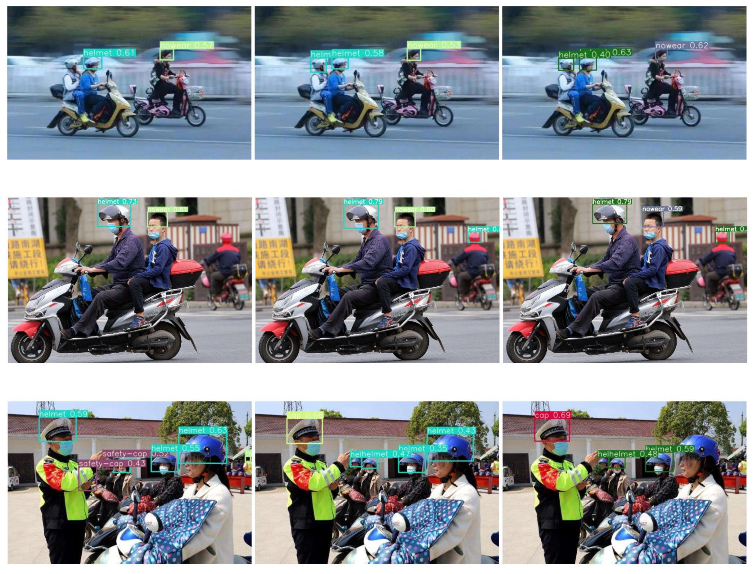
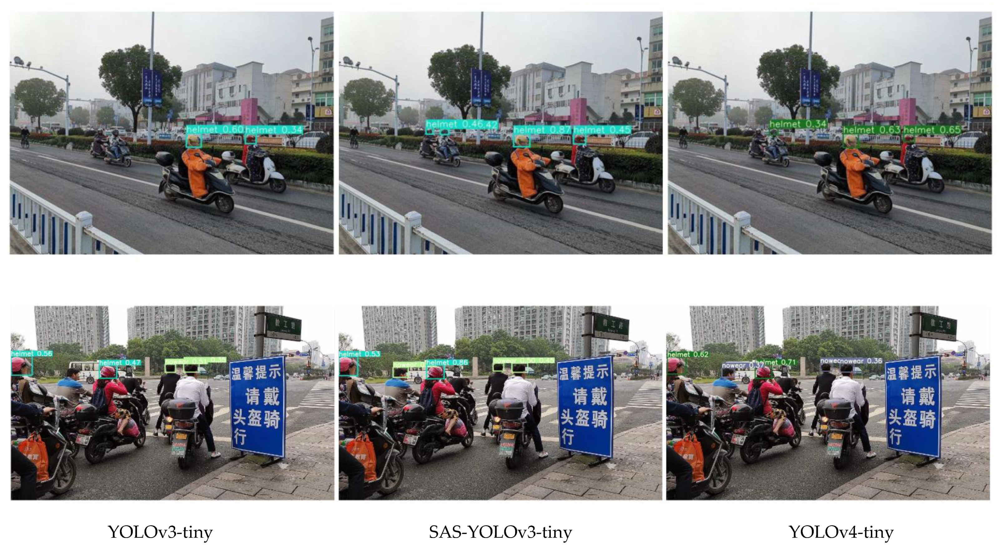
To prove that the improved algorithm is more suitable for natural complex scenes in terms of accuracy, we show the detection effect of some test images, which are shown in Figure 7. For small-scale objects, occluded objects and dense objects, SAS-YOLOv3-tiny is superior to the YOLOv3-tiny algorithm. As can be seen from the first and second set of images, SAS-YOLOv3-tiny and the latest YOLOv4-tiny can detect all objects, but YOLOv3-tiny leaves out an ordinary object. As can be seen from the third set of images, SAS-YOLOv3-tiny can detect all objects while YOLOv4-tiny neglects a helmet object, and YOLOv3-tiny detects some of the objects incorrectly. For detecting small objects at long distances, SAS-YOLOv3-tiny has better performance than YOLOv3-tiny and YOLOv4-tiny. In the last set of images, SAS-YOLO-v3-tiny and YOLOv4-tiny can detect some standard objects, but they will miss objects to be detected when a man deliberately lowers his head. As can be seen from the above test images, the improved algorithm is superior to the original algorithm and sometimes even has a better detection effect than the latest YOLOv4-tiny.

5. Conclusions

In this paper, the SAS-YOLOv3-tiny algorithm is proposed to solve the problem that the original lightweight algorithm YOLOv3-tiny was low at accuracy. Even though YOLOv3-tiny has a faster speed and fewer parameters, its detection accuracy needs to be improved. First of all, the lightweight Sandglass-Residual module based on depthwise separable convolution and channel attention mechanism was constructed to replace the original convolution layer while the max-pooling layer was replaced with the convolution layer of stride two, which could reduce the number of parameters and improve detection performance. Furthermore, the detection performance is further improved when three-scale feature prediction is utilized. Next, the improved spatial pyramid pooling module was merged behind the backbone network to extract expressive features. Finally, we utilized CIoU to improve the loss function, which also improved the location effect. In conclusion, for the validation set, SAS-YOLOv3-tiny made P from 70.7% to 73.2%, made R from 73.3% to 80.2%, made mAP from 73.7% to 81.6% and made F1 from 71.9% to 76.4%. For the test set, SAS-YOLOv3-tiny had good generalization, and it performed better than the original YOLOv3-tiny at the expense of 0.7 ms speed, which was comparable to YOLOv4-tiny in terms of detection accuracy; compared with the heavyweight algorithms YOLOv3 and YOLOv4, SAS-YOLOv3-tiny had a great advantage in speed although its detection accuracy was not as good as theirs. The experimental results and contrast curves reveal that the improved methods can strengthen the effect of detection. The next work is to expand the safety helmet dataset based on the dataset in this paper and further improve the detection accuracy while maintaining a lower number of parameters and speed.

Author Contributions

Conceptualization, X.H. and R.C.; methodology, R.C. and X.H.; software, R.C.; validation, X.H. and R.C.; formal analysis, X.H. and R.C.; investigation, R.C., X.H. and Z.W.; resources, X.H. and Z.Z.; data curation, R.C. and X.H.; writing—original draft preparation, R.C.; writing—review and editing, X.H. and R.C.; visualization, X.H. and R.C.; supervision, X.H.; project administration, X.H. and Z.Z.; funding acquisition, X.H. and Z.Z. All authors have read and agreed to the published version of the manuscript.

Funding

This research was funded by the National Natural Science Foundation of China (NSFC) (61572023, 61672467).

Institutional Review Board Statement

Not applicable.

Informed Consent Statement

Not applicable.

Data Availability Statement

Some or all data, models or code generated or used during the study are available from the corresponding author by request.

Conflicts of Interest

The authors declare no conflict of interest.

References

  1. Girshick, R.; Donahue, J.; Darrelland, T.; Malik, J. Rich Feature Hierarchies for Accurate Object Detection and Semantic Seg-mentation. In Proceedings of the IEEE Conference on Computer Vision and Pattern Recognition, Columbus, OH, USA, 24–27 June 2014. [Google Scholar]
  2. He, K.; Zhang, X.; Ren, S.; Sun, J. Spatial pyramid pooling in deep convolutional networks for visual recognition. IEEE Trans. Pattern Anal. Mach. Intell. 2015, 37, 1904–1916. [Google Scholar] [CrossRef] [PubMed] [Green Version]
  3. Girshick, R. Fast R-CNN. In Proceedings of the 2015 IEEE International Conference on Computer Vision (ICCV), Santiago, Chile, 7–13 December 2015; pp. 1440–1448. [Google Scholar]
  4. Ren, S.; He, K.; Girshick, R.; Sun, J. Faster R-CNN: Towards Real-Time Object Detection with Region Proposal Networks. IEEE Trans. Pattern Anal. Mach. Intell. 2017, 39, 1137–1149. [Google Scholar] [CrossRef] [Green Version]
  5. Dai, J.; Li, Y.; He, K.; Sun, J. R-FCN: Object Detection via Region-based Fully Convolutional Networks. In Proceedings of the Conference on Neural Information Processing Systems, Barcelona, Spain, 5–10 December 2016. [Google Scholar]
  6. Lin, T.-Y.; Dollar, P.; Girshick, R.; He, K.; Hariharan, B.; Belongie, S. Feature Pyramid Networks for Object Detection. In Proceedings of the 2017 IEEE Conference on Computer Vision and Pattern Recognition (CVPR), Honolulu, HI, USA, 21–26 July 2017; pp. 936–944. [Google Scholar]
  7. He, K.; Gkioxari, G.; Dollar, P.; Girshick, R.B. Mask R-CNN. IEEE Trans. Pattern Anal. Mach. Intell. 2020, 42, 386–397. [Google Scholar] [CrossRef] [PubMed]
  8. Sermanet, P.; Eigen, D.; Zhang, X.; Mathieu, M.; Fergus, R.; Lecun, Y. OverFeat: Integrated Recognition, Localization and Detection using Convolutional Networks. arXiv 2013, arXiv:1312.6229. [Google Scholar]
  9. Redmon, J.; Divvala, S.; Girshick, R.; Farhadi, A. You Only Look Once: Unified, Real-Time Object Detection. In Proceedings of the IEEE Conference on Computer Vision and Pattern Recognition, Las Vegas, NV, USA, 27–30 June 2016; pp. 779–788. [Google Scholar]
  10. Liu, W.; Anguelov, D.; Erhan, D.; Szegedy, C.; Reed, S.; Fu, C.Y. SSD: Single Shot Multi Box Detector. In Proceedings of the Europe Conference on Computer Vision, Amsterdam, The Netherlands, 8–16 October 2016; pp. 21–37. [Google Scholar]
  11. Lin, T.-Y.; Goyal, P.; Girshick, R.B.; He, K.; Dollar, P. Focal Loss for Dense Object Detection. IEEE Trans. Pattern Anal. Mach. Intell. 2020, 42, 318–327. [Google Scholar] [CrossRef] [PubMed] [Green Version]
  12. Redmon, J.; Farhadi, A. YOLO9000: Better, Faster, Stronger. In Proceedings of the 30th IEEE Conference on Computer Vision and Pattern Recognition, Honolulu, HI, USA, 21–26 July 2017; pp. 6517–6525. [Google Scholar]
  13. Redmon, J.; Farhadi, A. YOLOv3: An Incremental Scheme. In Proceedings of the IEEE Conference on Computer Vision and Pattern Recognition, Salt Lake City, UT, USA, 18–22 June 2018; pp. 1854–1862. [Google Scholar]
  14. Huang, L.; Yang, Y.; Deng, Y.; Yu, Y. DenseBox: Unifying Landmark Localization with End to End Object Detection. arXiv 2015, arXiv:1509. 04874. [Google Scholar]
  15. Law, H.; Deng, J. CornerNet: Detecting Objects as Paired Keypoints. Int. J. Comput. Vis. 2020, 128, 642–656. [Google Scholar] [CrossRef] [Green Version]
  16. Zhou, X.; Zhuo, J.; Krahenbuhl, P. Bottom-Up Object Detection by Grouping Extreme and Center Points. In Proceedings of the 2019 IEEE/CVF Conference on Computer Vision and Pattern Recognition (CVPR), Long Beach, CA, USA, 16–20 June 2019; pp. 850–859. [Google Scholar]
  17. Duan, K.; Bai, S.; Xie, L.; Qi, H.; Huang, Q.; Tian, Q. CenterNet: Keypoint Triplets for Object Detection. In Proceedings of the 2019 IEEE/CVF International Conference on Computer Vision (ICCV), Seoul, Korea, 27 October–2 November 2019; pp. 6568–6577. [Google Scholar]
  18. Zhu, C.; He, Y.; Savvides, M. Feature Selective Anchor-Free Module for Single-Shot Object Detection. In Proceedings of the 2019 IEEE/CVF Conference on Computer Vision and Pattern Recognition (CVPR), Long Beach, CA, USA, 16–20 June 2019; pp. 840–849. [Google Scholar]
  19. Tian, Z.; Shen, C.; Chen, H.; He, T. FCOS: Fully Convolutional One-Stage Object Detection. In Proceedings of the 2019 IEEE/CVF International Conference on Computer Vision (ICCV), Seoul, Korea, 27 October–2 November 2019; pp. 9626–9635. [Google Scholar]
  20. Kong, T.; Sun, F.; Liu, H.; Jiang, Y.; Li, L.; Shi, J. FoveaBox: Beyound Anchor-Based Object Detection. IEEE Trans. Image Process. 2020, 29, 7389–7398. [Google Scholar] [CrossRef]
  21. Wang, H.; Hu, Z.; Guo, Y.; Yang, Z.; Zhou, F.; Xu, P. A Real-Time Safety HelmetWearing Detection Approach Based on CSYOLOv3. Appl. Sci. 2020, 10, 6732. [Google Scholar] [CrossRef]
  22. Li, Y.; Wei, H.; Han, Z.; Huang, J.; Wang, W. Deep Learning-Based Safety Helmet Detection in Engineering Management Based on Convolutional Neural Networks. Adv. Civ. Eng. 2020, 2020, 1–10. [Google Scholar] [CrossRef]
  23. Sandler, M.; Howard, A.; Zhu, M.; Zhmoginov, A.; Chen, L.-C. MobileNetV2: Inverted Residuals and Linear Bottlenecks. In Proceedings of the 2018 IEEE/CVF Conference on Computer Vision and Pattern Recognition, Salt Lake City, UT, USA, 18–23 June 2018; pp. 4510–4520. [Google Scholar]
  24. Daquan, Z.; Hou, Q.; Chen, Y.; Feng, J.; Yan, S. Rethinking Bottleneck Structure for Efficient Mobile Network Design. arXiv 2020, arXiv:2007.02269. [Google Scholar]
  25. Hu, J.; Shen, L.; Albanie, S.; Sun, G.; Wu, E. Squeeze-and-Excitation Networks. In Proceedings of the 2018 IEEE Conference on Computer Vision and Pattern Recognition, Salt Lake City, UT, USA, 18–22 June 2018. [Google Scholar]
  26. Zheng, Z.; Wang, P.; Ren, D.; Liu, W.; Ye, R.; Hu, Q.; Zuo, W. Enhancing Geometric Factors in Model Learning and Inference for Object Detection and Instance Segmentation. arXiv 2020, arXiv:2005.03572. [Google Scholar]
  27. Rezatofighi, H.; Tsoi, N.; Gwak, J.; Sadeghian, A.; Reid, I.; Savarese, S. Generalized Intersection Over Union: A Metric and a Loss for Bounding Box Regression. In Proceedings of the 2019 IEEE/CVF Conference on Computer Vision and Pattern Recognition (CVPR), Long Beach, CA, USA, 15–20 June 2019; Institute of Electrical and Electronics Engineers (IEEE): Piscataway, NJ, USA, 2019; pp. 658–666. [Google Scholar]
  28. Zheng, Z.; Wang, P.; Liu, W.; Li, J.; Ye, R.; Ren, D. Distance-IoU Loss: Faster and Better Learning for Bounding Box Regression. 2019, pp. 1458–1467. Available online: https://arxiv.org/abs/1911.08287 (accessed on 9 March 2020).
  29. Bochkovskiy, A.; Wang, C.Y.; Liao, H.Y.M. YOLOv4: Optimal Speed and Accuracy of Object detection. arXiv 2020, arXiv:2004.10934. [Google Scholar]
  30. Wang, C.-Y.; Liao, H.-Y.M.; Wu, Y.-H.; Chen, P.-Y.; Hsieh, J.-W.; Yeh, I.-H. CSPNet: A New Backbone that can Enhance Learning Capability of CNN. In Proceedings of the IEEE/CVF Conference on Computer Vision and Pattern Recognition Workshops, Glasgow, UK, 23–28 August 2020; pp. 390–391. [Google Scholar]
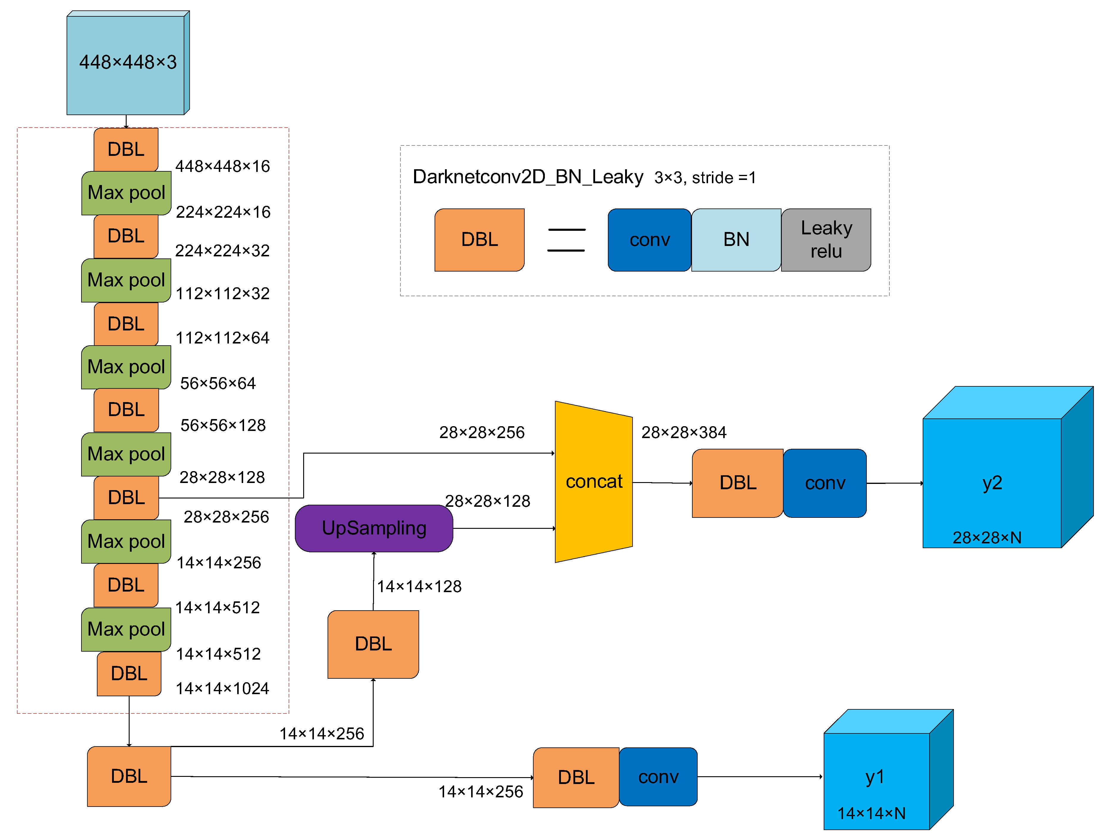
Figure 1. YOLOv3-tiny network structure.
Applsci 11 03652 g001
Figure 2. The final bounding box prediction schematic.
Applsci 11 03652 g002
Figure 3. Sandglass-Residual module based on the Squeeze-Excitation channel attention.
Applsci 11 03652 g003
Figure 4. Improved spatial pyramid pooling module.
Applsci 11 03652 g004
Figure 5. SAS-YOLOv3-tiny network structure.
Applsci 11 03652 g005
Figure 6. The curves of F1 and mAP in the different models.
Applsci 11 03652 g006
Figure 7. The detection results of some test images.
Applsci 11 03652 g007aApplsci 11 03652 g007b
Table 1. The parameters of Sandglass-Residual module.
InputOperationOutput
h × w × n 3 × 3 Dwise conv, leaky h × w × n
h × w × n 1 × 1 conv, linear h × w × n 2
h × w × n 2 1 × 1 conv, leaky h × w × n
h × w × n 3 × 3 Dwise conv, linear h × w × n
Table 2. Different improvement schemes.
SchemeSR3-ScaleSPPSECIoU
SR
SR-3s
SR-3s-SPP
SR-3s-SPP-SE
SR-3s-SPP-SE-CIoU(Ours)
Table 3. Ablation results of different models on the validation set.
ModelP/%R/%mAP/%F1/%Weight/MBTotal
Parameters/106
Detection Time/ms
YOLOv3-tiny70.773.373.771.969.58.676812.5
SR69.377.978.273.336.54.534902.8
SR-3s69.679.680.274.239.24.866583.0
SR-3s-SPP70.380.480.175.045.45.653013.1
SR-3s-SPP-SE72.380.281.276.046.95.827733.2
SR-3s-SPP-SE-CIoU(Ours)73.280.281.676.446.95.827733.2
Table 4. Comparison of different algorithms for object detection on the test set.
AlgorithmType
Helm-etAP/
Cap
%
Nowear
Safey-
Cap
P/%R/%mAP/%F1/%Weight/MBTotal
Parameters/107
Detection Time/ms
YOLOv3-tiny70.974.076.277.571.075.474.672.969.50.867682.5
YOLOv4-tiny80.474.780.879.872.680.078.976.047.20.587791.8
YOLOv384.281.292.586.675.885.686.180.3492.86.153998.6
YOLOv486.780.992.789.379.488.687.483.7420.75.247987.4
SAS-YOLOv3-tiny78.273.387.881.971.680.980.375.246.90.582773.2
Publisher’s Note: MDPI stays neutral with regard to jurisdictional claims in published maps and institutional affiliations.