Article

Required Moment Sets: Enhanced Controllability Analysis for Nonlinear Aircraft Models

Institute of Flight System Dynamics, Technical University of Munich, 85748 Garching bei München, Germany
*
Author to whom correspondence should be addressed.
Appl. Sci. 2021, 11(8), 3456; https://doi.org/10.3390/app11083456
Submission received: 5 March 2021 / Revised: 28 March 2021 / Accepted: 2 April 2021 / Published: 12 April 2021
(This article belongs to the Special Issue Aerospace System Analysis and Optimization)

Abstract

:

Featured Application

The developed methods can be used in aircraft configuration design and optimization along with controller design. The main application is requirements-based propulsive control sizing for multirotor and distributed electric propulsion aircraft configurations.

Abstract

Attainable moment sets (AMS) are a powerful method to assess aircraft controllability. However, as attainable moment sets only take into account the achievable moment set of the control effectors, they do not assess the required moment set to fulfill the aircraft mission requirements. This paper proposes to calculate a corresponding required moment set (RMS) which defines a set of moments sufficient for fulfilling aircraft controllability requirements in the mission flight envelope. The paper applies the required moment set approach to a nonlinear simulation model of an electric vertical take off vehicle (eVTOL) transition drone in hover. By comparing the required moment set to the AMS of the aircraft model, moment set margins are derived and used to assess the controllability of the considered aircraft. The results indicate that the combined evaluation directly identifies critical moment channels and margins, which is advantageous when compared to a pure AMS-based evaluation. The proposed approach enables the execution of simulation-based assessments in aircraft design and flight control development. In the early stages of aircraft design, required moment sets can support sizing, positioning and tilting of control effectors (e.g., propulsive elements) to fit the AMS to the actual required force and moment set for the specific system.

1. Introduction

Recently, multirotor configurations have become popular, especially in urban air mobility applications [1]. A very common method to assess the controllability of these multirotor aircraft is the so-called attainable moment set (AMS), which is defined as the set of maximum moments that an aircraft can reach by using the full control authority [2,3]. The initial work on the concept of the AMS was motivated from a control allocation background [2,3] and the method was derived for linear systems. A method which enables the applicability to nonlinear systems was investigated in [4]. A more novel trim and optimization-based method for calculating a nonlinear AMS was developed in [5]. After the AMS is calculated, a very important question is also how to judge the controllability of the given AMS. The work in [6] proposes AMS shape criteria to make judgments about the controllability.
A disadvantage of these AMS-based controllability assessments is that they do not take into account what forces/moments are required to fulfill the aircraft mission requirements within the desired envelope. Especially for transition capable multicopter configurations that are also supposed to obtain wingborne flight, the aerodynamic effective surfaces can cause high disturbance moments in hover mode which should be considered when evaluating the controllability via an AMS.
For this reason, this paper proposes to evaluate a required moment set (RMS), which is a set containing the worst case required moments that need to be covered by the attainable moments in order for the aircraft to fulfill controllability requirements. Consequently, the RMS defines a minimum required AMS which can be used to assess and even to optimize the actual AMS of the vehicle, e.g., by tilting propulsive elements or sizing propulsive units.
The main objective of this paper is to present methods to obtain a measure of controllability based on attainable and required control sets. As the AMS has already been studied thoroughly in current literature, this work’s objective is to mainly focus on the RMS and to allow a direct comparison of AMS and RMS. As the proposed methods shall be applicable already in early stages of aircraft design, the used methods shall rely only on aircraft simulation models. Another very important objective is the traceability of RMS subsets, i.e., to be able to distinguish between different parts of the RMS, e.g., parts to obtain angular accelerations and parts to trim against aerodynamic disturbances.
After this introduction, the paper focuses on the methods used to achieve above mentioned objectives. In a first step, the RMS is split up conceptually in different required parts, e.g., for maneuvering and for countering aerodynamic disturbances. As the proposed approach is based on a simulation model, the underlying physical assumptions as well as equations are presented. In a next step we derive a method to numerically evaluate the required moment set for aerodynamic disturbances. In order to guarantee a straightforward comparison of AMS and RMS the following subsection deals with the assembly in a convex hull-based control set. In order to complete the different types of control sets, the required control set and the attainable set are investigated as well. Finally a method to assess the controllability is shown. The paper then finishes with results for a transition capable multirotor configuration and derives conclusions about the applicability of the methods to achieve the above specified objectives.

2. Materials and Methods

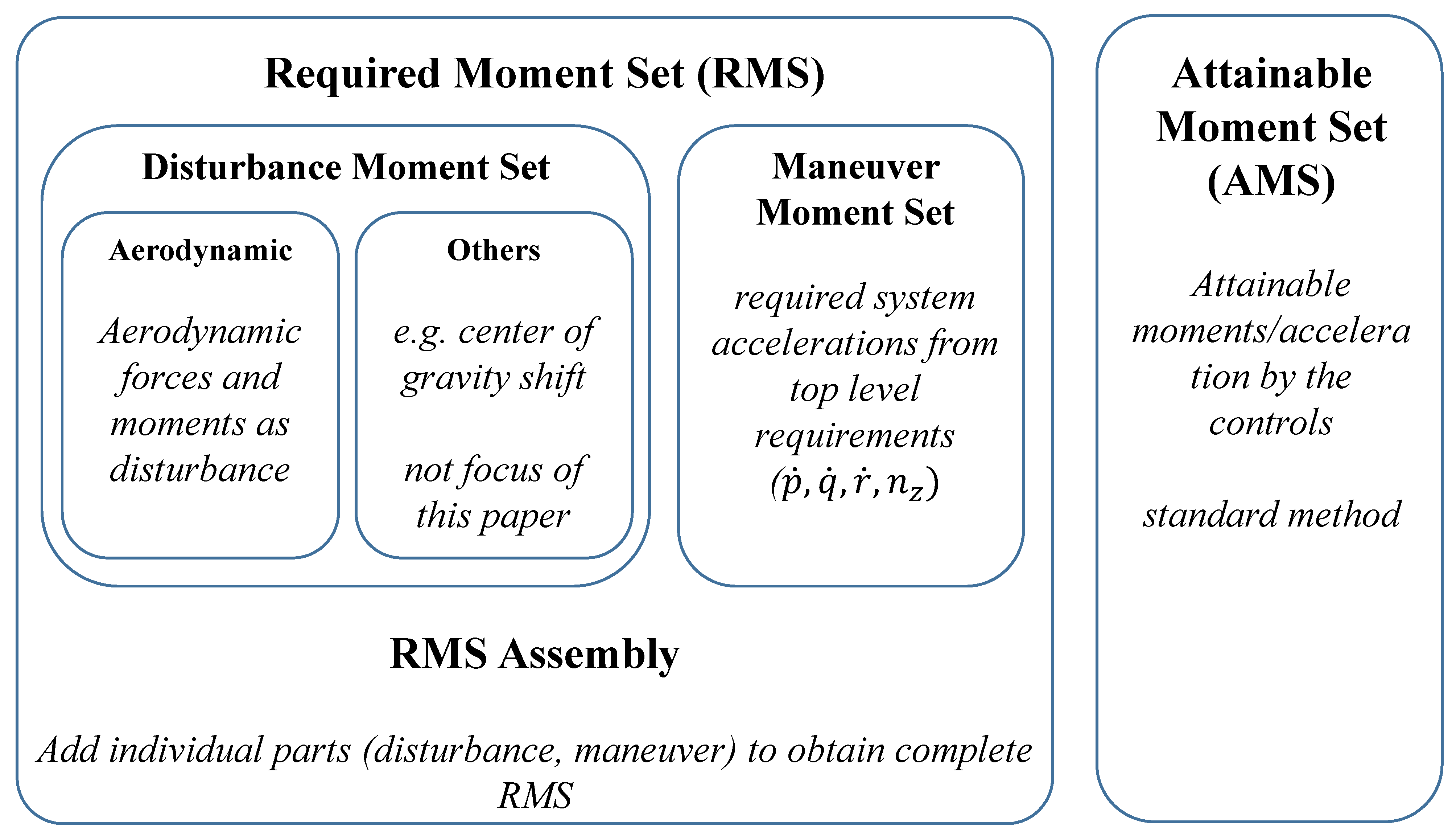
2.1. Separation Into Individual Required Control Subsets

In order to calculate the required moment set in a structured manner and in order to perform the proposed RMS-based controllability assessment in a traceable manner, the required forces and moments are split into individual subsets. We call the first part the disturbance part, which constitutes the required propulsive forces and moments that are required to counter disturbances. This paper focuses on the aerodynamic disturbance, as in hover mode the aerodynamic forces and moments have to be compensated for via the propulsive system and are not part of the flight control as they are for wingborne mode.
In order to determine the maximum possible aerodynamic disturbance that can act during the operation, the aircraft is first trimmed at the boundary points of the aerodynamic velocity envelope, as there the aerodynamic disturbance obtains the highest magnitudes. In all possible trimmed directions of flight, multiple attitude deviations from the trim points are used to evaluate aerodynamic forces and moments. With this approach we obtain a realistic set of possible aerodynamic forces and moments that need to be countered by the propulsive system.
For the sake of simplicity the calculation process and moment set approach include a configuration with a fixed direction of hover thrust (no tilt configuration); for this reason, the required moment set is defined by the three roll, pitch and yaw moments ( L , M , N ) or corresponding angular accelerations ( p ˙ , q ˙ , r ˙ ) and the total aircraft thrust in the body z-direction T or the corresponding body z load factor ( n z ) B .
Figure 1 shows an overview of the different parts of the required moment set that is used throughout this paper. Besides countering aerodynamic disturbance, the propulsive system also needs to provide the desired maneuverability. The corresponding desired quantities are attainable accelerations (angular and translational), which from a kinematic point of view and provide sufficient dynamics for fulfilling higher level mission requirements. We use the angular body accelerations ( p ˙ , q ˙ , r ˙ ) and the inertial translational acceleration in the body z direction ( a z ) B as direct requirements. These acceleration limits again define a convex set (e.g., a four dimensional cube).
In order to sum up the disturbance and maneuverability parts of the required forces/ moments, we use query directions in the four-dimensional set space and find the cross sections with the convex hull of the corresponding sets. This procedure simplifies the summation process of disturbance and maneuverability sets, which finally yields the full set of required forces/moments.
In order to finally assess the controllability, the attainable and required control sets need to be compared. To evaluate this, first the AMS is calculated by applying all possible combinations of minimum or maximum propulsive inputs and assembling them in a convex set [7,8]. In a second step, the convex set intersections in the direction of the query directions are determined. Afterwards, attainable and required forces/moments are available in the same query directions and can be directly compared to assess the controllability margins and to identify critical directions/channels.

2.2. Underlying Aircraft Simulation Model

The use of a simulation model-based assessment can be applied already in early aircraft design and can help lower development costs. One of the main applications of aircraft simulation models is model-based control design as in [9,10]. In order to guarantee a close match to the real aircraft system, identification can be used to improve the accuracy of the models [11,12].
To demonstrate the RMS approach with the methods of this paper, a simulation model of a lift and cruise multirotor UAV is used. As the methods used in this paper do not require time simulation, this section only shows the force and moment balance parts of the equations of motion. The translational and rotational equations of motion read [13].
u ˙ K G v ˙ K G w ˙ K G B I I = 1 m X A G Y A G Z A G B + 1 m X P G Y P G Z P G B + sin ( Θ ) cos ( Θ ) sin ( Φ ) cos ( Θ ) cos ( Φ ) B g ,
p ˙ q ˙ r ˙ = ( I B B G ) 1 L A G M A G N A G B + ( I B B G ) 1 L P G M P G N P G B ( I B B G ) 1 p q r B × I B B G p q r B ,
where u , v , w denote the three velocity components, K the kinematic nature, G the center of gravity, the index I I the inertial acceleration, m the vehicle mass, X , Y , Z and L , M , N forces and moments due to aerodynamics A or propulsion P. The inertia around the center of gravity in the body frame is denoted with I B B G .
In order to provide an aerodynamic model for flow from all possible directions, a multi-compartment aerodynamic model comparable to [14] is used. Assembling all forces and moments in the center of gravity then yields
X A G Y A G Z A G B = 1 2 ρ V A 2 S r e f C X ( α A , β A ) C Y ( α A , β A ) C Z ( α A , β A ) B ,
L A G M A G N A G B = 1 2 ρ V A 2 S r e f s C l ( α A , β A ) c ¯ C m ( α A , β A ) s C n ( α A , β A ) B ,
where S r e f denotes the wing reference area, s the wing span, c ¯ the chord, V A the magnitude of the true airspeed and C i the force/moment coefficients. The dependency of the coefficients with respect to the aerodynamic angle of attack α A and angle of sideslip β A are realized with lookup tables [15].
The multirotor propulsion system is modeled independent of the aerodynamics; propulsion airframe interactions are neglected. For each propulsive unit, the propeller forces and moments are modelled as linear in the squares of the angular rates [16,17]
T i = C T D 4 ρ 1 4 π 2 ω i 2 ,
N i = C N D 5 ρ 1 4 π 2 ω i 2 ,
where T i denotes the thrust of the ith propeller, N i the corresponding torque around the corresponding rotational axis, ω i the rotational rate in rad/s and D the propeller diameter. As the aircraft only has propellers of the same type the thrust coefficient C T and the torque coefficient C N are the same for all propellers.

2.3. Trim-Based Calculation of Aerodynamic Disturbance Set

Now that an aircraft model is established, a very important next objective of this paper is to establish means to calculate different parts of required control sets. This section explains the proposed method of calculating the worst case aerodynamic disturbance throughout the aircraft mission.
The presented analysis is carried out for a given altitude h and density of the atmosphere ρ 
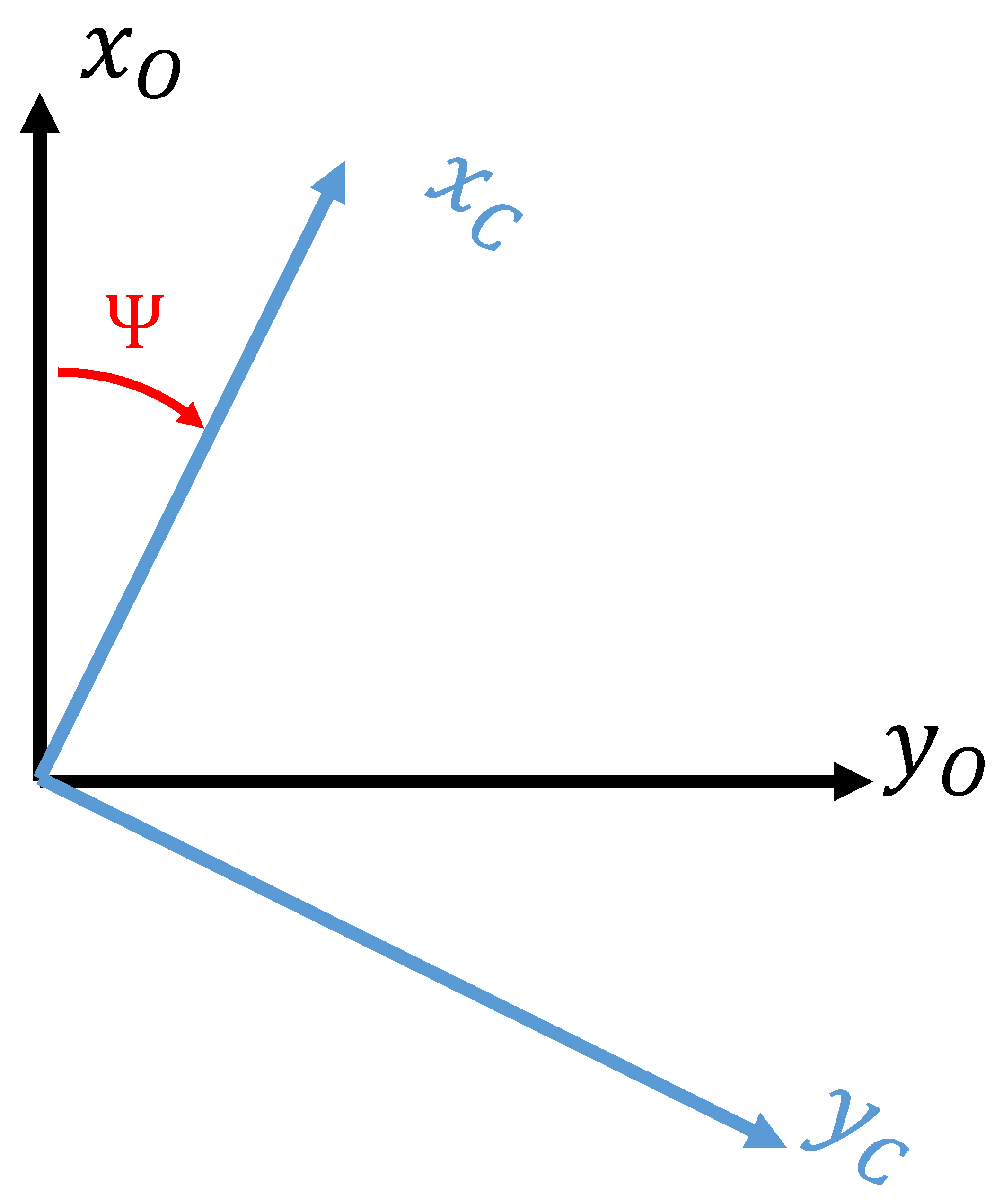
. At this point the aircraft is required to be able to fly up to certain kinematic speeds in various directions. A convenient frame to describe the three-dimensional velocities is the control frame C as it is indifferent to the heading Ψ but includes the down direction [18]. Figure 2 shows the axes of the C-frame.
Besides the kinematic speed requirement, there can also be requirements for environmental conditions such as wind speeds. Combining both requirements yields a total airspeed envelope that the vehicle must be able to cover. For the sake of simplicity let us assume a cuboidal envelope of the shape
u C , m i n u C u C , m a x ,
v C , m i n v C v C , m a x ,
w C , m i n w C w C , m a x ,
with u C , v C , w C denoting the components of the aerodynamic velocity given in the C frame V C 3 × 1 .
For all points within this airspeed envelope the aircraft must be able to obtain steady state operation. In order for the aircraft to be in steady state attitude, the body rates ( p , q , r ) and the corresponding accelerations ( p ˙ , q ˙ , r ˙ ) need to be zero. The translational motion of the aircraft is then defined by the velocity point in the envelope V C . The total hover thrust of the aircraft T tilted by the attitude ( Φ , Θ ) needs to offset the aerodynamic and gravitational forces in order to reach no translational acceleration and steady state velocities in the C frame. For the sake of simplicity it is assumed that the hover thrust direction coincides with the negative body z direction which yields the force trim balance equation
X A ( Θ , Φ , V C ) Y A ( Θ , Φ , V C ) Z A ( Θ , Φ , V C ) B + 0 0 T + sin ( Θ ) cos ( Θ ) sin ( Φ ) cos ( Θ ) cos ( Φ ) m g = ! 0 0 0 .
Note that for applying this method an aerodynamic model defining X A , Y A , Z A ( Θ , Φ , V C ) over the full envelope of angles of attack and angles of sideslip is required. As these models are nonlinear, Equation (10) needs to be solved numerically, e.g., via Matlab’s fsolve() [19] or more aircraft tailored trim solutions [20].
In order to determine the maximum possible aerodynamic disturbance hull, only the boundary of the aerodynamic velocity envelope is considered, as the dynamic pressure and therefore also possible disturbance forces/moments reach their highest values here, see Figure 3. As individual points are required for the moment set and assembly to a convex hull, we selected a number of query points that represents our envelope boundary. Unlike for simplified approaches when calculating an AMS where the number of set points is finite, for this nonlinear aerodynamic disturbance set the number of points can be chosen to be arbitrarily large. Higher resolution in the query points on the envelope boundary will increase the accuracy of the obtained RMS but also increase the amount of points that need to be analyzed. The later Results section will show the results for different chosen resolutions of the RMS.
As the mission hover envelope in most cases follows simple geometrical shapes (e.g., cuboid or ellipsoid) in the control frame, the points can be chosen as linearly spaced on the boundary. Let n V denote the number of representative points on the boundary of the airspeed envelope. Figure 3 shows exemplary representative query points in 2D for an ellipsoidal required aerodynamic velocity envelope.
As the operation of the aircraft is considered around a steady trim state and during the transition from one trim state to another trim state, the aircraft is trimmed at all n V query points using Equation (10). The aerodynamic forces and moments in these trim points already constitute one part of the disturbance moment set. However, as we are also interested in transitions/maneuvers from one trim state to another (e.g., acceleration or deceleration in the lateral direction), the disturbance for these maneuvers is calculated as well.
In order to account for these maneuvers, we assume that, at each trim point, the attitude of the aircraft can vary from the trim point while the airspeed is kept constant. In order to model the transition phases and the obtained aerodynamic inflow angles realistically without being too conservative, a range of attitude deviation from the trim point obtainable via maneuvers is determined. For this, minimum and maximum allowed attitude angles for maneuvers can be derived from system requirements. Additionally, an overshoot over the trim pitch/roll angles is allowed in order to make the disturbances more realistic. Figure 4 shows the idea of the attitude variation for an exemplary 2D model. In the range of the minimum and maximum pitch and roll angles, different attitude deviations/combinations from the trim point are calculated. The allowed attitude region follows
Φ = min ( Φ m i n , Φ t r i m Φ o v e r s h o o t ) ,
Φ + = max ( Φ m a x , Φ t r i m + Φ o v e r s h o o t ) ,
Θ = min ( Θ m i n , Θ t r i m Θ o v e r s h o o t ) ,
Θ + = max ( Θ m a x , Θ t r i m + Θ o v e r s h o o t ) .
As for the query points on the boundary of the velocity envelope, query points in the bounded Φ - Θ -plane are used to obtain set points for various inflow angles during maneuvers from one trim state to another. Let n Φ , Θ denote the total number of points in the attitude plane. Note that the maneuver disturbance here follows from attitude deviations and body rates are neglected for the sake of reducing computational complexity.
The corresponding required moments to counter the disturbances follow by evaluating the aerodynamic model at the n Φ , Θ query attitude points with the query inflow
L R M S , D M R M S , D N R M S , D B = L A ( Θ , Φ , V C ) M A ( Θ , Φ , V C ) N A ( Θ , Φ , V C ) B ,
where the index D denotes the disturbance part. The requirement for the total propulsive thrust to compensate for the disturbances depends on the desired behavior during the maneuver. We considered transitions in the horizontal plane, as these transitions change the attitude/inflow angles, and therefore there will be arbitrary accelerations depending on the attitude in the horizontal direction. In the vertical direction, however, the propulsive system needs to counter the disturbance (e.g., negative lift of the wing when hovering forward with negative pitch angle). This requires a total zero force in the z direction of the control frame. Transforming the force balance Equation (10) into the C frame and taking the z component yields
sin ( Θ ) X A ( Θ , Φ , V C ) + cos ( Θ ) sin ( Φ ) Y A ( Θ , Φ , V C ) + cos ( Θ ) cos ( Φ ) Z A ( Θ , Φ , V C ) cos ( Θ ) cos ( Φ ) T + m g = 0 .
Solving for the thrust leads to
T R M S , D = Z A ( Θ , Φ , V C ) tan ( Θ ) cos ( Φ ) X A ( Θ , Φ , V C ) + tan ( Φ ) Y A ( Θ , Φ , V C ) + m g cos ( Θ ) cos ( Φ ) .
In order to have a more scale-free and kinematic judgment of the controllability configuration we transform the forces/moments to resulting accelerations and assemble the moment set points in the acceleration space. The rotational accelerations follow from the rotational equations of motion
p ˙ R M S , D q ˙ R M S , D r ˙ R M S , D B = ( I B B G ) 1 L R M S , D M R M S , D N R M S , D B .
The translational equations of motion lead to
( n z , R M S , D ) B = T R M S , D m g .
This yields all angular and translational accelerations at the n V n Φ , Θ total query points for different envelope boundary points as well as attitude deviations. The next section explains how to assemble these points and combine them with other required moments in a convex hull approach.

2.4. Convex Hull-Based Control Set Assembly

The last subsection contributed to the objective of calculating clearly traceable parts of the RMS. This subsection proposes a method to add these individual RMS subsets and to compare them to the AMS. After the query points for the disturbance set are assembled, the convex hull [7] of the set can be computed in order to obtain a worst case estimation of the aerodynamic disturbance. Note that this convex hull-based approach is chosen here as it can be performed generically for any set of points regardless of the physical origin. An efficient algorithm for determining the convex hull of an arbitrary set of points is the quickhull algorithm [8], which is implemented in the Matlab function convhulln(). It is important to mention here that, due to the nonlinearities in the aerodynamic coefficients, the aerodynamic disturbance set is in general no convex set. The goal of this paper, however, is a comparison of the RMS with the AMS. For this reason, assembling the RMS as a convex set does not produce overly conservative results. Any convex AMS that contains a non-convex RMS will also contain a more conservative convex version of the RMS.
In order to be able to sum up the different independent elements of the RMS (disturbance and maneuverability parts) and compare them to the AMS, we propose to calculate the maximum attainable acceleration in the query directions of the four-dimensional acceleration space. This reduces computational effort and produces magnitudes in predefined directions that do not depend on the configuration but are chosen by the user. This approach also allows comparison of different configurations with respect to each other very easily. A disadvantage of this method is that for small numbers of query directions, the actual set might not be resolved accurately enough. In order to resolve the moment set with higher accuracy, the number of query directions increases very fast as the moment set is four-dimensional.
The maximum of the accelerations in the query directions is determined by the points in the query direction that lie on the convex hull. An efficient algorithm to determine the cross sections with the convex is presented in [21].
To parameterize the four-dimensional directions, we use an n-spherical coordinate system [22] which, for the four-dimensional case, requires three angles for the parameterization. Including a scaling along the four-dimensions which leads to
d n z = n z , s c a l e cos ( β 1 )
d p ˙ = p ˙ s c a l e sin ( β 1 ) cos ( β 2 )
d q ˙ = q ˙ s c a l e sin ( β 1 ) sin ( β 2 ) cos ( β 3 )
d r ˙ = r ˙ s c a l e sin ( β 1 ) sin ( β 2 ) sin ( β 3 )
d = 1 d n z 2 + d p ˙ 2 + d q ˙ 2 + d r ˙ 2 d n z d p ˙ d q ˙ d r ˙ ,
with the normalized query direction d R 4 × 1 and the three parameterization angles β 1 , β 2 [ 0 . . . π ] and β 3 [ 0 . . . 2 π ) . As for the velocity envelope and the attitude deviation, we again use linearly spaced parameterization angles. Let n β 1 , n β 2 , n β 3 denote the number of the corresponding angles for the linear spacing, then n β = n β 1 n β 2 n β 3 is the total number of query directions. Finally, all directions are assembled in a direction matrix D R 4 × n β .
Applying this query direction approach to the convex hull obtained from the aerodynamic disturbance moments in all directions contained in D and assembling the results in a row vector yields the required acceleration magnitudes for disturbance rejection a R M S , D R 1 × n β .

2.5. Calculation of Required Maneuver Set and Assembly of Total Required Set

The last subsection yielded a query direction-based control set interface which can be used to easily add and compare control sets. This section will focus on the required control set to maneuver the aircraft in order to complete the total required moment set.
The required moment set for maneuvering can be expressed in terms of maximum accelerations that are used by the system to fulfill higher level missions/maneuvers. In a possible controller architecture, these maximum accelerations could be implemented as limitations/protections. In the case of an individual channel limitation a cuboidal convex set is obtained, defined by
( Δ n z , m a x ) B ( Δ n z , R M S , D ) B ( Δ n z , m a x ) B
p ˙ m a x p ˙ R M S , M p ˙ m a x
q ˙ m a x q ˙ R M S , M q ˙ m a x
r ˙ m a x r ˙ R M S , M r ˙ m a x .
For the required maneuverability set above, the cross sections in the acceleration directions can directly be obtained via first finding the critical surface of the cuboid by applying an elementwise division of the direction d and the critical limits in the corresponding channels and taking the maximum value. Scaling up the direction vector d by the inverse of this value will lead to hitting the boundary of the cuboid; therefore, the inverse of the value is the cross section magnitude in this direction
a R M S , M = 1 max d ( Δ n z , m a x ) B p ˙ m a x q ˙ m a x r ˙ m a x ,
where ⊘ and | | denote the elementwise division and absolute value, respectively. Applying Equation (29) to all directions in D and assembling the results in a row vector yields the required acceleration magnitudes for maneuverability a R M S , M R 1 × n β . To obtain the total required accelerations we now can simply add maneuver and disturbance accelerations
a R M S = a R M S , D + a R M S , M .

2.5.1. Evaluation of Attainable Moment Set

In order to finally perform a control set-based controllability analysis, the attainable control set needs to be calculated and transformed to the query direction-based control set interface. There are methods for evaluating the attainable moments for nonlinear control effector models [5]. For the exemplary multirotor electric vertical take off vehicle (eVTOL) configurations that are the focus of this paper, simplified propellers with thrust and propeller torque that is linear in the squares of the angular propeller rates are used. For this reason the attainable set can be obtained by evaluating the angular and translational accelerations of all combinations of minimum and maximum propeller angular rates. The corresponding convex hull can again be found by using the quickhull algorithm [8].
In general, the proposed approach allows more complex nonlinear propeller models for calculating the AMS as well. It is important to mention here that the comparison with the RMS does not allow an inflow dependent AMS, as the RMS is chosen for the worst case inflow in the envelope. A possible solution to this problem is to also choose the worst case AMS via intersecting multiple AMSs that were calculated at different points in the aerodynamic velocity envelope.
After the convex hull is calculated, the same approach as for the required moments is used to assemble the intersections in the query directions in the vector a A M S R 1 × n β .

2.5.2. Controllability Evaluation

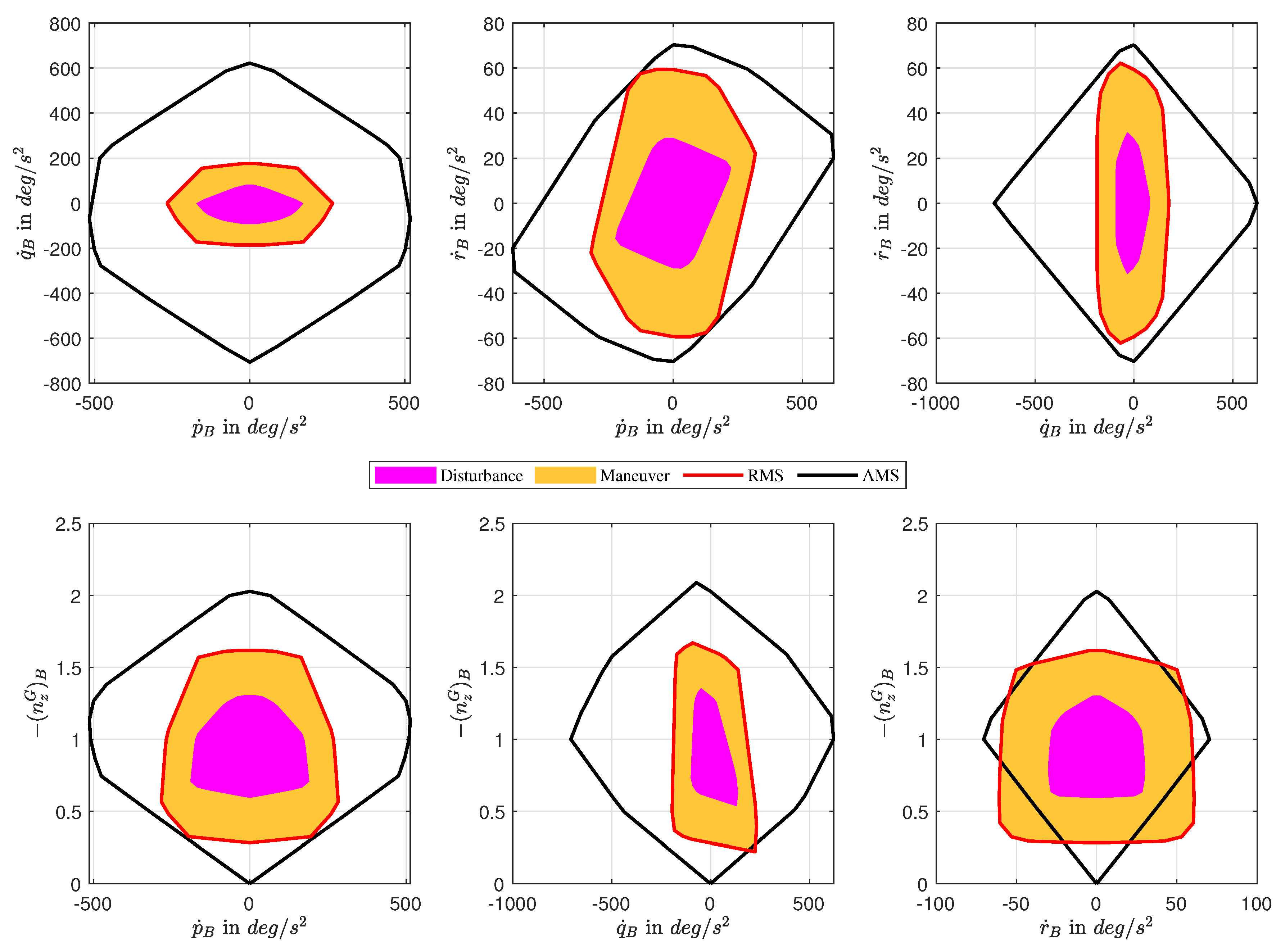
Now that attainable and required acceleration sets are determined, the easiest way to assess the controllability is just to check if, in any direction, the required moment set exceeds what is attainable:
min ( a A M S a R M S ) 0 . .
According to this definition, Equation (31) is a condition for fulfilling the controllability requirements. Note that this simple comparison contributes to two major objectives of this paper. First of all, a very simple final evaluation of controllability is possible. Second of all, the RMS is obtained from a simple sum of individual sets, therefore it is always traceable what the corresponding contributions of individual sets are.
In order to obtain continuous instead of binary controllability measures we can assemble a margin vector, which contains the differences of attainable and required accelerations. In order to obtain a more relative controllability measure, the margin can be normalized by the required moment set that obtains a relative margin vector m R 1 × n β .
m = ( a A M S a R M S ) a A M S .
In order to assess the overall controllability, various norms can be used to transform the vector margin to a scalar controllability measure.

3. Results

This section investigates the results obtained from the described analysis carried out for the above specified model of a transition eVTOL configuration. Figure 5 shows the results for the RMS and AMS acceleration set.
The chosen discretization numbers were ( n u = 5 , n v = 5 , n w = 5 , n Φ = 10 , n Θ = 10 , n β 1 = 12 , n β 2 = 12 , n β 3 = 24 ), the airspeed envelope was defined via ( u C , m i n = 8 m/s, v C , m i n = 8 m/s, w C , m i n = 3 m/s, u C , m a x = 8 m/s, v C , m a x = 8 m/s, w C , m a x = 3 m/s,), the maneuver attitude deviations were ( Φ m i n = 20 deg, Φ m a x = 20 deg, Θ m i n = 20 deg, Θ m a x = 20 deg, Φ o v e r s h o o t = 5 , Θ o v e r s h o o t = 5 ), the scales were chosen to ( n z , s c a l e = 2 , p ˙ s c a l e = 1000 deg/s2, q ˙ s c a l e = 1000 deg/s2, r ˙ s c a l e = 120 deg/s2) and the maneuverability limitations were chosen to ( Δ n z , m a x = 3 / g m/s2, p ˙ m a x = 90 deg/s2, q ˙ m a x = 90 deg/s2, r ˙ m a x = 30 deg/s2).
For visualization we chose the six possible pair combinations of the four chosen acceleration channels and plotted the cross section of the corresponding channel pair plane with the hull defined via the query directions lying in the plane. This visualization provides a very fast and intuitive understanding of possible problematic directions. The purple area represents the maximum possible aerodynamic disturbance accelerations while the orange areas on top are the additional accelerations corresponding to required maneuverability. The sum of both yields the total RMS (red line). As the right bottom yaw/body z acceleration plot in Figure 5 shows, we can immediately identify the critical directions of requirement violation. The cuboid shape of the maneuverability required moment set leads to higher required moments than the AMS can provide in cases of simultaneous yaw and body z acceleration demands. The controllability evaluation taking into account the RMS also shows clear advantages over the solely AMS-based evaluation here, as it directly identifies the critical direction that would not be available for a purely AMS-based evaluation.
Another important effect which needs to be investigated when assessing the proposed methods is the effect of resolutions for calculating the control sets. The first important resolution to mention here is the number of chosen query directions to span the control sets n β 1 , n β 2 , n β 3 . Table 1 shows the controllability analysis results for different chosen values corresponding to 3.75°, 7.5°, 15° and 30° resolution.
To assess the controllability, three measures are shown. The first two measures are the minimum and mean value of the control set margins from Equation (32). The third measure is the percentage of control set query directions for which the attainable control is not greater or equal than required control m < 0 . Decreasing the control set resolution down to 3.75° also increases the accuracy of the controllability measures.
Another important resolution effect to investigate is the chosen resoultion of bank and pitch angles when evaluating the disturbance set. Table 2 shows the controllability analysis results for various resoultions in the pitch and bank angle plane.
When the corresponding resolution is increased, all three controllability measures converge. This shows that the method of assembling the aerodynamic disturbance set points via linearly spacing is suitable to obtain worst case estimates of the aerodynamic disturbance for the given simulation model.

4. Conclusions

The results indicate that the calculation of a required moment set allows an intuitive controllability analysis based on system requirements. The assembly in a control set enables a simple comparison of AMS and RMS and at the same time keeps traceability of a source of a required moment (e.g., aerodynamic disturbance or maneuverability). The resolution analysis of control sets showed the convergence of simple measures of controllability when the underlying resolutions are increased. Consequently, the methods for assembling the aerodynamic disturbance set points and the query direction-based intersection set assembly are able to cover the full control set area. However, the price of a high accuracy of the presented results are higher computation times as the number of query directions rises with third power of the underlying resolution.
As the introduced RMS and calculation approach were only carried out in an exemplary manner for a considered eVTOL, refinements can be investigated in the future. For example, disturbance sources such as center of gravity and mass uncertainties can be included in the disturbance moment set as well. At the same time, means to include the effect of body rates on the disturbance forces/moments can be analyzed in future work. Another important aspect to mention here is the inclusion of model uncertainties in order to obtain probabilistic controllability statements. To obtain probabilistic judgements, the uncertainties first need to be quantified [23] and then included in the simulation model [15]. It is important to mention here that the inclusion of sample-based stochastic analysis will further increase the computation times and therefore requires an efficient algorithmic implementation.
As this work mainly focuses on the introduction and calculation of the RMS, it opens various options to use the RMS, e.g., in design optimization and controller design. For design optimization, suitable measures based on the presented controllability margins can be investigated. For control design for a given configuration, the allowable airspeed envelope can be determined which guarantees sufficient maneuverability. Additionally, given a desired airspeed envelope, the maximum available maneuverability can be determined, which can be used for protective measures in flight control algorithms.

Author Contributions

Conceptualization, M.S. and J.Z.; methodology, M.S.; software, M.S.; validation, M.S. and J.Z.; investigation, M.S.; writing—original draft preparation, M.S.; writing—review and editing, N.B.; visualization, M.S.; supervision, F.H.; project administration, F.H.; funding acquisition, F.H. All authors have read and agreed to the published version of the manuscript.

Funding

This research received no external funding.

Institutional Review Board Statement

Not applicable.

Informed Consent Statement

Not applicable.

Data Availability Statement

Data sharing not applicable.

Conflicts of Interest

The authors declare no conflict of interest.

Abbreviations

The following abbreviations and nomenclature are used in this manuscript:
eVTOLElectric Vertical Take Off Vehicle
AMSAttainable Moment Set
RMSRequired Moment Set
Ψ , Θ , Φ Euler angles (heading, pitch, roll)
β spherical coordinates for acceleration set parameterization
Aindex for aerodynamic forces/moments
BBody frame
CControl frame
ONorth–East–Down frame
D query direction matrix
I B B G inertia tensor around the center of gravity, given in the body frame
L , M , N moment components
Thover thrust
V aerodynamic velocity vector
X , Y , Z force components
a acceleration magnitudes in query directions
d query direction vector
ggravitational acceleration
m relative set margins
maircraft mass
n z load factor in z-direction
p , q , r body angular rates
u , v , w aerodynamic velocity components

References

  1. Polaczyk, N.; Trombino, E.; Wei, P.; Mitici, M. A Review of Current Technology and Research in Urban On-Demand Air Mobility Applications. In Proceedings of the 8th Biennial Autonomous VTOL Technical Meeting and 6th Annual Electric VTOL Symposium, Mesa, AZ, USA, 29–31 January 2019. [Google Scholar]
  2. Durham, W.C. Attainable Moments for the Constrained Control Allocation Problem. J. Guid. Control. Dyn. 1994, 17, 1371–1373. [Google Scholar] [CrossRef]
  3. Durham, W.C. Constrained Control Allocation-Three-Moment Problem. J. Guid. Control. Dyn. 1994, 17, 330–336. [Google Scholar] [CrossRef]
  4. Bolender, M.; Doman, D. Method for Determination of Nonlinear Attainable Moment Sets. J. Guid. Control. Dyn. 2004, 27, 907–914. [Google Scholar] [CrossRef]
  5. Varriale, C.; Voskuijl, M.; Veldhuis, L.L. Trim for Maximum Control Authority using the Attainable Moment Set. In Proceedings of the AIAA Scitech 2020 Forum, Orlando, FL, USA, 6–10 January 2020; p. 1265. [Google Scholar]
  6. Kim, K.; Rahili, S.; Shi, X.; Chung, S.J.; Gharib, M. Controllability and Design of Unmanned Multirotor Aircraft Robust to Rotor Failure. In Proceedings of the AIAA Scitech 2019 Forum, San Diego, CA, USA, 7–11 January 2019; p. 1787. [Google Scholar]
  7. Brondsted, A. An Introduction to Convex Polytopes; Springer Science & Business Media: New York, NY, USA, 2012; Volume 90. [Google Scholar]
  8. Barber, C.B.; Dobkin, D.P.; Huhdanpaa, H. The Quickhull Algorithm for Convex Hulls. ACM Trans. Math. Softw. 1996, 22, 469–483. [Google Scholar] [CrossRef] [Green Version]
  9. Raab, S.A.; Zhang, J.; Bhardwaj, P.; Holzapfel, F. Proposal of a Unified Control Strategy for Vertical Take-Off and Landing Transition Aircraft Configurations. In Proceedings of the 2018 Applied Aerodynamics Conference, Atlanta, GA, USA, 25–29 June 2018; p. 3478. [Google Scholar]
  10. Dul, F.; Lichota, P.; Rusowicz, A. Generalized Linear Quadratic Control for a Full Tracking Problem in Aviation. Sensors 2020, 20, 2955. [Google Scholar] [CrossRef] [PubMed]
  11. Lichota, P. Multi-Axis Inputs for Identification of a Reconfigurable Fixed-Wing UAV. Aerospace 2020, 7, 113. [Google Scholar] [CrossRef]
  12. Göttlicher, C.; Gnoth, M.; Bittner, M.; Holzapfel, F. Aircraft Parameter Estimation Using Optimal Control Methods. In Proceedings of the AIAA Atmospheric Flight Mechanics Conference, San Diego, CA, USA, 4–8 January 2016; p. 1534. [Google Scholar]
  13. Boiffier, J.L. The Dynamics of Flight; American Institute of Aeronautics and Astronautics: New York, NY, USA, 1998. [Google Scholar]
  14. Selig, M. Modeling Full-Envelope Aerodynamics of Small UAVs In Realtime. In Proceedings of the AIAA Atmospheric Flight Mechanics Conference, Toronto, ON, Canada, 13–16 August 2010; p. 7635. [Google Scholar]
  15. Bähr, N.M.; Soepper, M.M.; Holzapfel, F. Stochastic Lookup Tables-A Method for the Integration of Parametric Uncertainties in Non-Linear Simulation Models. In Proceedings of the AIAA Scitech 2021 Forum, Nashville, TN, USA, 19–21 January 2021; p. 0545. [Google Scholar]
  16. Leishman, G.J. Principles of Helicopter Aerodynamics with CD Extra; Cambridge University Press: Cambridge, UK, 2006. [Google Scholar]
  17. Johnson, W. Helicopter Theory; Courier Corporation: Mineola, NY, USA, 2012. [Google Scholar]
  18. Bhardwaj, P.; Raab, S.A.; Zhang, J.; Holzapfel, F. Thrust Command Based Integrated Reference Model with Envelope Protections for Tilt-rotor VTOL Transition UAV. In Proceedings of the AIAA Aviation 2019 Forum, Dallas, TX, USA, 17–21 June 2019; p. 3266. [Google Scholar]
  19. Coleman, T.F.; Li, Y. An Interior Trust Region Approach for Nonlinear Minimization Subject to Bounds. SIAM J. Optim. 1996, 6, 418–445. [Google Scholar] [CrossRef] [Green Version]
  20. Weingartner, M.; Lenz, J.; Sachs, G.; Holzapfel, F. Object Oriented Trim of Complex High-Fidelity Simulation Models. In Proceedings of the AIAA Modeling and Simulation Technologies Conference and Exhibit, Hilton Head, SC, USA, 20–23 August 2007; p. 6704. [Google Scholar]
  21. Zhang, J.; Söpper, M.; Holzapfel, F. Attainable Moment Set Optimization to Support Configuration Design: A Required Moment Set Based Approach. J. Appl. Sci. 2021, in press. [Google Scholar]
  22. Blumenson, L. A Derivation of n-Dimensional Spherical Coordinates. Am. Math. Mon. 1960, 67, 63. [Google Scholar] [CrossRef] [Green Version]
  23. Lim, D.; Li, Y.; LeVine, M.J.; Kirby, M.; Mavris, D.N. Parametric uncertainty quantification of aviation environmental design tool. In Proceedings of the 2018 Multidisciplinary Analysis and Optimization Conference, Atlanta, GA, USA, 25–29 June 2018; p. 3101. [Google Scholar]
Figure 1. Overview of required and attainable moment sets and the proposed methods for obtaining the required moment set.
Applsci 11 03456 g001
Figure 2. Visualization of the Control frame C, which is a North–East–Down frame O, rotated by the heading Ψ around the z-axis.
Applsci 11 03456 g002
Figure 3. Exemplary distribution of boundary points on the aerodynamic velocity envelope in the control frame (2D example for visualization purposes).
Applsci 11 03456 g003
Figure 4. Illustration of attitude deviation for calculating disturbance moments and forces during maneuvers (2D example for visualization purposes).
Applsci 11 03456 g004
Figure 5. Results of the calculation of attainable moment set (AMS) and required moment set (RMS) hulls.
Applsci 11 03456 g005
Table 1. Controllability Analysis Results For Different Query Point Resolutions.
ResolutionMean (m)Min (m)Failure Percentage
n β 1 = n β 2 = 6 , n β 3 = 12 0.391 0.298 18.52 %
n β 1 = n β 2 = 12 , n β 3 = 24 0.391 0.367 15.50 %
n β 1 = n β 2 = 24 , n β 3 = 48 0.398 0.369 14.94 %
n β 1 = n β 2 = 48 , n β 3 = 96 0.403 0.371 14.69 %
Table 2. Controllability Analysis Results For Different Disturbance Set Resolutions.
ResolutionMean (m)Min (m)Failure Percentage
n ϕ = 2 , n θ = 2 0.414 0.318 14.04 %
n ϕ = 5 , n θ = 5 0.399 0.365 14.83 %
n ϕ = 10 , n θ = 10 0.398 0.369 14.94 %
n ϕ = 20 , n θ = 20 0.397 0.370 14.96 %
n ϕ = 40 , n θ = 40 0.397 0.370 14.97 %
n ϕ = 80 , n θ = 80 0.397 0.370 14.97 %
Publisher’s Note: MDPI stays neutral with regard to jurisdictional claims in published maps and institutional affiliations.

