An Integrated Thermal-Electrical Model for Simulations of Battery Behavior in CubeSats

Abstract

This work presents an integrated thermal-electrical simulation model, capable of taking into account the thermal and electrical effects of the battery and photovoltaic panels for each instant of time in a given orbit and attitude. Using the physical equations that govern the thermal and electrical models involved during a CubeSat operation, the proposed integrated model can estimate the temperature and energy conditions of the battery, not only in an isolated way but also in considering the mutual effects on the system. Besides, special attention is given to photovoltaic panels used in the energy harvesting process, whose performance is affected by irradiance and temperature along the orbit. The integrated model can be useful for engineers when developing the subsystems of their CubeSats, taking into account, for example, the battery temperature control through a heater. Simulations were performed to illustrate the functioning of the proposed model with variations in the power requirements of its modules and the temperature of the battery throughout the orbit, and a heater’s influence on it.

1. Introduction

As a result of electronic miniaturization, compact and light platforms were projected for space applications, including the CubeSat standard proposed in 1999 [1]. In parallel to that, the introduction of CubeSat standard and COTS components reduced the price to put a small satellite in orbit by sharing the costs of a launch with multiple CubeSats as piggyback payloads, enabling universities and private companies worldwide to undertake technology demonstration missions in outer space at affordable prices and sustainable business models dedicated to CubeSats. Ten CubeSats were launched in 2000 and 297 in 2017; 458 launches are expected in 2020, and 2500 new CubeSats expected by 2025. The projections are that around 49% of them will be from private initiatives, 32% from universities, 5% from space agencies, and 4% from militaries [2].

A CubeSat is usually covered by photovoltaic panels (PV) on its surface to recharge the batteries and power the subsystems. However, due to the solar panels’ small size and volume, the energy harvesting capability heavily depends on its attitude concerning the Sun [3]. Additionally, as a consequence of the attitude, other parameters of great concern in CubeSats are PV and battery temperatures. While extreme cold and hot scenarios damage these parts and other electronic components, the optimum PV and battery performance only exists in a narrow range of temperature [4,5]. Therefore, the energy efficiency and harvested energy distribution are critical for the CubeSat missions, especially when the CubeSat cannot efficiently maintain its attitude towards the solar rays [6]. In this sense, a fundamental challenge in CubeSat missions is to cope with the shortage of available energy to power its subsystems throughout the satellite’s lifetime through simulations.

A battery’s life cycle is a function of diverse factors, mainly: the state of charge (SoC), the temperature, the charge/discharge current, and the end of charge voltage (EOCV). As a rule of thumb, a lower SoC means a worse life cycle, and the lower the temperature field, the charge/discharge current, and the EOCV, the better the cycle life [7,8]. Additionally, the batteries’ internal resistance shows a strong temperature dependence, increasing for low temperatures and impacting the CubeSat voltage drops and the mission’s power budget. Usually, the operational temperature recommended for batteries in CubeSat applications is between 253 and 333 K [9]. However, as experimentally demonstrated in [5], typical COTS batteries for CubeSat missions are Li-ion cells, whose energy storage capacity may be around 20% of its maximum (at 293 K) when exposed to 253 K. The “Mars Cube One” (MarCO) CubeSat is a good example where temperature control is a major challenge. The two MarCO CubeSats had Li-ion batteries kept within 273 to 303 K during all mission phases. Heaters attached to the battery were used to sustain the temperature, and passive materials were employed to allow heat exchanging with other satellite parts [10,11].

Similarly to the battery, the PV degradation in orbit is a function of the conditions in space, such as irradiance temperature field [3,4,12]. Only a fraction of the solar spectrum is useful for energy generation. The larger wavelengths of radiation are harmful for its operation because they heat the cells and reduce the photovoltaic effect’s efficiency, which is hardly ever above 30% [13]. Therefore, for efficient operation, a PV panel must avoid high levels of temperature and low irradiance. However, the desire for high radiation levels to generate more energy in solar cells contradicts the inherent rise in PV panels’ temperature by this effect itself. The authors in [14] tested solar cells, and they measured a drop of 3% in the efficiency for temperatures ranging from 280 to 320 K—the hottest temperature and the worst performance. The work of [15] measured a coefficient of loss of around 0.5% per degree.

By observing the above findings, a thermal simulation is essential for the proper prediction of PV operation in orbit, and it should include the satellite’s dynamics. When proposing a control methodology for a battery’s temperature using a heater, the most common method, the engineer must have access to an integrated thermal and electrical methodology. As observed in the work of [16], a purely numerical simulation has limitations in the depth of insight into the satellite’s real performance. However, it is a crucial tool for satellite development at design phases. Its implementation costs are attractive compared to hardware simulations and may be refined with experimental results to provide more accurate results.

Examples of CubeSats’ thermal simulations are found in [17,18,19], whose authors solved the transient temperature of critical components of the satellite, such as the battery, but the simulations neither had active thermal control nor integration with electrical models of the satellite. On the other hand, the work of [7] studied the state of charge estimation for the battery of satellites, but the authors did not assess it considering typical transient irradiance and temperature profiles found in orbit. There are also papers in the literature concerning specifically the design and management of satellites’ power systems (electrical models) [20,21,22,23,24,25]; however, they do not present any generalized method that CubeSat engineers can further develop in order to satisfy the mission constraints and requirements that they are focused on in that moment.

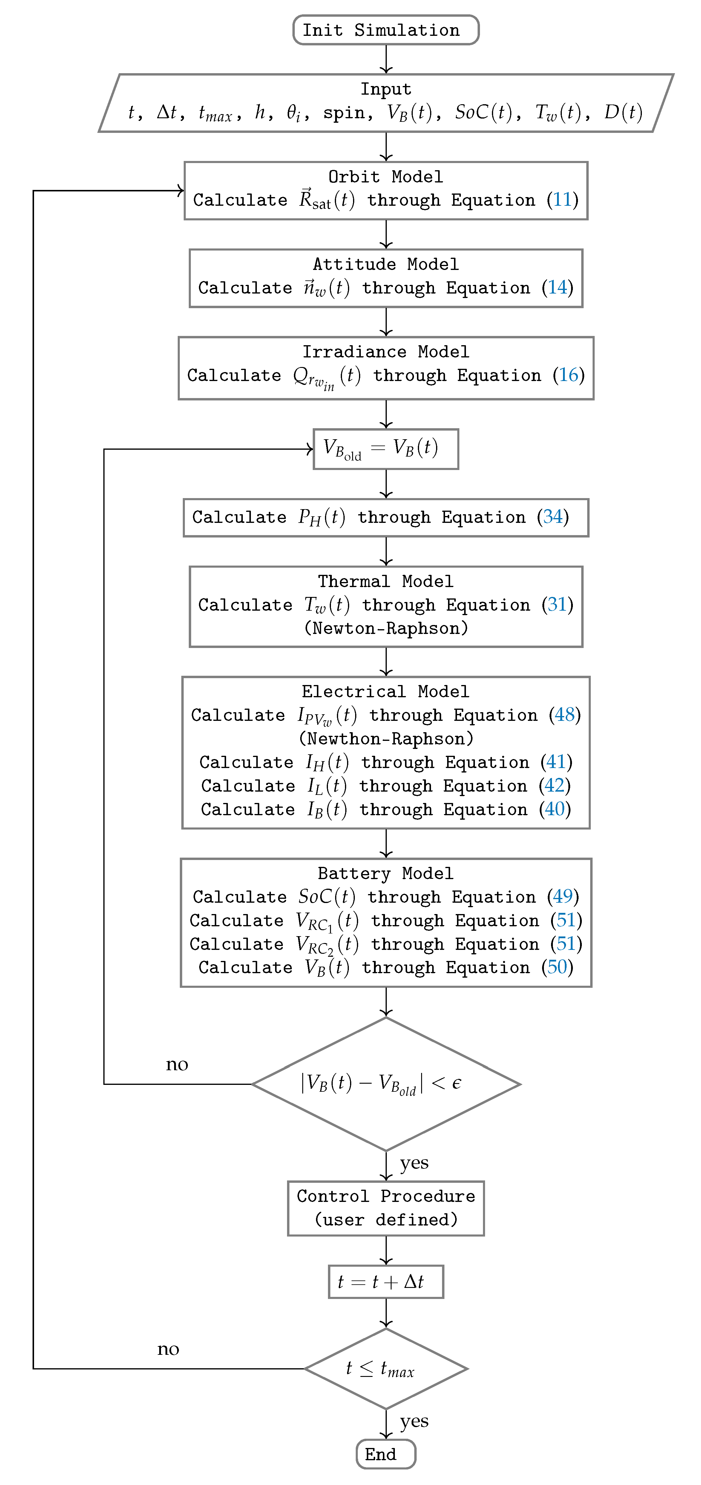
In this regard, this work presents an integrated thermal-electrical framework capable of taking into account the thermal and electrical effects of the battery and photovoltaic panels for each instant of time in a given orbit. In this way, the operator can evaluate the effects of a proposed thermal control on the battery’s temperature by turning on a heater and visualizing the effects of the solar panels’ varying temperatures during the orbit. It is also possible to assess the battery charge status due to the power to keep the heater activated.

Therefore, this work’s main contribution is an integrated and self-contained model for orbit, attitude, irradiance, thermal, electrical, and battery models for CubeSat mission analysis, especially useful for readers without access to commercial software for simulation of satellites. The model is versatile enough to simulate the thermal and electrical behavior under diverse types of orbit and attitude, including user-defined control dynamics, and does not require external simulators.

This paper is divided as follows: Section 2 presents the methodology to calculate the thermal and electrical parameters along the orbit; those equations are used to compose an integrated model presented in Section 3; simulation results are described in Section 4; the final remarks about the paper are drawn in Section 5.

2. Methodology

Initially, this section introduces the equations employed to model the CubeSat position in orbit and the satellite orientation. The transient irradiance and thermal balance are then described for a CubeSat geometry with a battery inside the satellite and six photovoltaic panels (PV) covering the external surfaces. In the sequence, the adopted electrical model includes the architecture of the satellite’s electrical power system (EPS), the solar panels, the battery, and its coupling with thermal parameters.

The models presented in this section are subjected to the following assumptions:

• Circular orbit without perturbations;
• One node is attributed for each part of the satellite, namely, six PV ($w=\left[1,2,3,4,5,6\right]$) and a battery ($w=7$);
• One normal vector will represent the orientation of each PV;
• PV does not generate heat;
• Thermal resistance among the solar panels is infinite;
• Every PV panel exchanges heat with the battery;
• Gray surfaces (absorptivity equal to emissivity);
• Constant material properties;
• Perfect vacuum condition;
• Experimental results regarding the battery internal losses are available.

2.1. Orbit Model

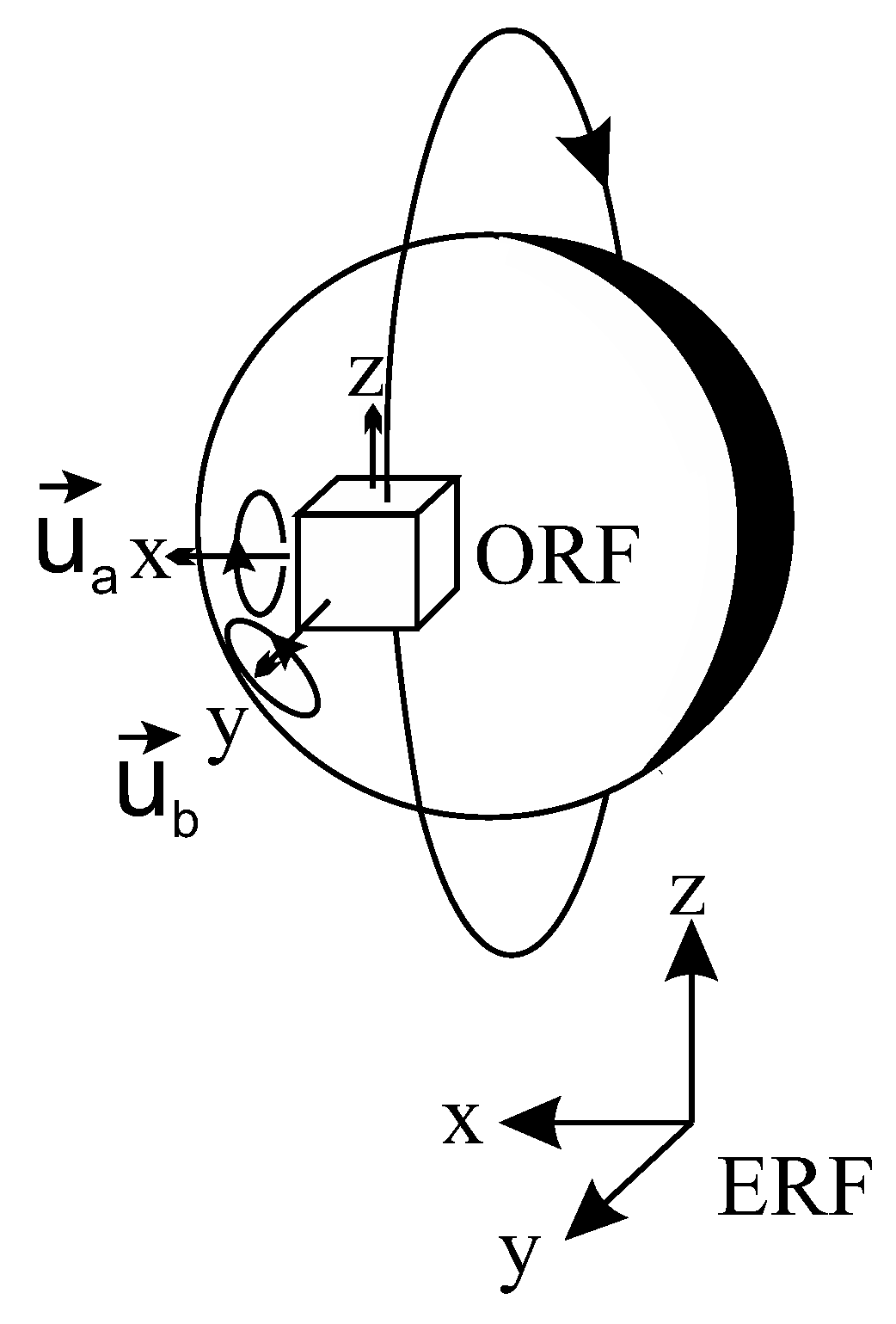
The orbit and the following attitude, irradiance, and thermal models generalize the previous work presented in [17]. An inertial Cartesian coordinate system called Earth Reference Frame (ERF) is centered on the Earth, and a non-inertial reference system named Orbit Reference Frame (ORF) is at the satellite’s center of mass. The y-component of the ERF points to the Sun ($\overrightarrow{S}=\left[0,1,0\right]$), the z-component to the celestial north pole, and the x-component is the cross product between them. The vector ${\overrightarrow{R}}_{sat}$ connects ORF to the origin of ERF, and defines the satellite’s position as a function of the angles in Figure 1.

The rotation matrix in Equation (1) is used to rotate a vector over one arbitrary axis.

$$\left[G\right]=\left[\begin{array}{ccc}{b}_{11}& b_{12}& b_{13}\\ b_{21}& b_{22}& b_{23}\\ b_{31}& b_{32}& b_{33}\end{array}\right]$$

(1)

where:

$$\begin{array}{cc}\hfill & b_{11}=cos\left(\theta \right)+u_1^2\left(1-cos\left(\theta \right)\right)\hfill \end{array}$$

(2)

$$\begin{array}{cc}\hfill & b_{12}=u_1{u}_2\left(1-cos\left(\theta \right)\right)-u_{3}sin\left(\theta \right)\hfill \end{array}$$

(3)

$$\begin{array}{cc}\hfill & b_{13}=u_1{u}_3\left(1-cos\left(\theta \right)\right)+u_{2}sin\left(\theta \right)\hfill \end{array}$$

(4)

$$\begin{array}{cc}\hfill & b_{21}=u_2{u}_1\left(1-cos\left(\theta \right)\right)+u_{3}sin\left(\theta \right)\hfill \end{array}$$

(5)

$$\begin{array}{cc}\hfill & b_{22}=cos\left(\theta \right)+u_2^2\left(1-cos\left(\theta \right)\right)\hfill \end{array}$$

(6)

$$\begin{array}{cc}\hfill & b_{23}=u_2{u}_3\left(1-cos\left(\theta \right)\right)-u_{1}sin\left(\theta \right)\hfill \end{array}$$

(7)

$$\begin{array}{cc}\hfill & b_{31}=u_3{u}_1\left(1-cos\left(\theta \right)\right)-u_{2}sin\left(\theta \right)\hfill \end{array}$$

(8)

$$\begin{array}{cc}\hfill & b_{32}=u_3{u}_2\left(1-cos\left(\theta \right)\right)+u_{1}sin\left(\theta \right)\hfill \end{array}$$

(9)

$$\begin{array}{cc}\hfill & b_{33}=cos\left(\theta \right)+u_3^2\left(1-cos\left(\theta \right)\right)\hfill \end{array}$$

(10)

$\theta$ is the angle of rotation around the unitary vector with components $\overrightarrow{u}=[u_1,u_2,u_3]$. For a satellite with spin, $\theta =\omega t$, where $\omega$ and t are the angular speed and time, respectively. The satellite’s position (${\overrightarrow{R}}_{\mathrm{sat}}$) results from the combination of different rotation matrices in sequence.

Two matrices will be used here, representing the orbit inclination ($\left[M_i\right]$) and the translational progress in the orbital plane ($\left[M_j\right]$), respectively, as in the next equation:

$${\overrightarrow{R}}_{\mathrm{sat}}=\left[M_j\right]\left[M_i\right]{\overrightarrow{R}}_{\mathrm{sat},0}$$

(11)

The subscript 0 represents the first satellite’s position, given by ${\overrightarrow{R}}_{\mathrm{sat},0}=[0,h+R_e,0]$ in the ERF, where h is the altitude and $R_e$ the Earth’s radius (6378 km). The unit vector inside the matrix $\left[M_j\right]$ must be perpendicular or co-linear to the solar vector $\overrightarrow{S}$ to reproduce orbits with or without eclipse, respectively. The angle to mimic the translation of the satellite around the Earth is given by:

$${\theta }_j\left(t\right)={\omega }_{e}t=\sqrt{\frac{m_{e}K}{{\left(R_e+h\right)}^3}}t,$$

(12)

From this equation, valid for circular orbit, ${\omega }_e$ is the satellite’s angular speed around the Earth, K is the gravitational constant ($6.674\times {10}^{-11}$ m${}^3$/kg s${}^2$), and $m_e$ is the Earth’s mass ($5.972\times {10}^{24}$ kg) [26].

2.2. Attitude Model

There will be six main external surfaces in a CubeSat without deployable solar panels, whose orientations are described by their normal vectors (${\overrightarrow{n}}_w$). Similarly to the previous section, their inclination may be defined by other two angles, now around the ORF. Figure 2 illustrates the axes of the rotational matrix, the position, and orientation of the CubeSat at the first step in orbit.

Two rotational matrices will be used to simulate the attitude models of this work, as follows:

$$\begin{array}{cc}\hfill & {\overrightarrow{n}}_w^{*}\left(t\right)={\left[M_a\right]}_{\mathrm{ERF}}{\overrightarrow{n}}_{w,0}\hfill \end{array}$$

(13)

$$\begin{array}{cc}\hfill & {\overrightarrow{n}}_w\left(t\right)={\left[M_b\right]}_{\mathrm{ORF}}{\overrightarrow{n}}_w^{*}\hfill \end{array}$$

(14)

In the first step, the six CubeSat’s sides rotate around the axis ${\overrightarrow{u}}_a$ at the angle $\Delta {\theta }_a$. After that, the satellite suffers one more rotation, now around the axis ${\overrightarrow{u}}_b$, at the angle $\Delta {\theta }_b$. The inclinations after this last rotation (${\overrightarrow{n}}_w$) are ${\overrightarrow{n}}_{w,0}$ at the next iteration $it+1$. For a spin in two axes, the first rotation will be around a fixed axis at the ERF, and the second will occur around the transient axis ${\overrightarrow{n}}_w^{*}\left(t\right)$ at the ORF.

2.3. Irradiance Model

The net radiation heat rate ($Q_{r_w}$) expresses the radiation heat exchange of the CubeSat’s external surfaces, which depends on the orientation of the surface w. For each surface w, except $w=7$, there is incoming radiation ($Q_{r_{w_{\mathrm{in}}}}$) given by the direct absorbed radiation from the Sun ($Q_{\mathrm{Sun}}$), radiation absorbed from the reflections off the Earth’s surface called albedo ($Q_{\mathrm{alb}}$), and absorbed infrared radiation emitted by the Earth ($Q_{\mathrm{IR}}$) [27]. There is still energy emission ($Q_{r_{w_{\mathrm{out}}}}$) from the satellite’s surfaces to outer space ($Q_{\mathrm{sat}\to \mathrm{spa}}$), as shown in:

$$Q_{r_w}\left(t\right)=Q_{r_{w_{\mathrm{in}}}}\left(t\right)-Q_{r_{w_{\mathrm{out}}}}\left(t\right)$$

(15)

Or:

$$Q_{r_{w_{in}}}\left(t\right)=Q_{{\mathrm{Sun}}_w}\left(t\right)+Q_{{\mathrm{alb}}_w}\left(t\right)+Q_{{\mathrm{IR}}_w}\left(t\right)$$

(16)

$$Q_{r_{w_{\mathrm{out}}}}\left(t\right)=Q_{{\mathrm{sat}}_w\to spa}\left(t\right)$$

(17)

Equation (15) is a boundary condition of the thermal problem, which requires thermal parameters and also variables from the orbit and attitude models. The terms in Equations (16) and (17) are:

Solar radiation: It is the primary heat source for satellites in Low Earth Orbit (LEO). In this work, the solar flux radiation ($Q_{\mathrm{Sun}}^{\prime \prime }$) is constant, and the solar rays are parallel. Equation (18) estimates the total radiation absorbed from the Sun.

$$Q_{{\mathrm{Sun}}_w}^{\prime \prime }\left(t\right)={\alpha }_w{A}_{r_w}{Q}_{s_w}^{\prime \prime },$$

(18)

where:

$$Q_{s_w}^{\prime \prime }\left(t\right)=F_{w\to \mathrm{Sun}}\left(t\right)\xi \left(t\right)Q_{\mathrm{Sun}}^{\prime \prime }$$

(19)

In these equations, ${\alpha }_w$ is the surface’s absorptivity of the satellite, $A_{r_w}$ is the external area of each side w, $F_{w\to \mathrm{Sun}}$ is the view factor between the surface w and the Sun, and $\xi$ is a step function to account for the eclipse, so it assumes the value 0 when the satellite is under the shadow of the Earth and 1 when it is outside. Both $F_{w\to \mathrm{Sun}}\left(t\right)$ and $\xi \left(t\right)$ are functions of the attitude and orbit models, respectively. The view factor between the surface w and the Sun is calculated by Equation (20), which is basically the projection of that surface towards the Sun, while $\xi$ is estimated by Equation (21), based on Figure 3.

$$F_{w\to \mathrm{Sun}}\left(t\right)=|min\left({\overrightarrow{n}}_w\left(t\right).\overrightarrow{S},0\right)|$$

(20)

$$\xi \left(t\right)=\left\{\begin{array}{cc}0,\hfill & {cos}^{-1}\left(\frac{{\overrightarrow{R}}_{\mathrm{sat}}\left(t\right).\overrightarrow{S}}{|{\overrightarrow{R}}_{\mathrm{sat}}\left(t\right)\left|·\right|\overrightarrow{S}|}\right)\ge {tan}^{-1}\left(\frac{R_e}{R_e+h}\right)+\frac{\pi }{2}\hfill \\ 1,\hfill & \mathrm{otherwise}\hfill \end{array}\right.$$

(21)

Albedo radiation: defined by Equation (22), it is the amount of radiation from the Sun that hits the Earth’s surface and reflects back to outer space.

$$Q_{{\mathrm{alb}}_w}\left(t\right)=a{\alpha }_w{A}_{r_w}{F}_{w\to e}\left(t\right)U\left(t\right)Q_{\mathrm{Sun}}^{\prime \prime }$$

(22)

The term a is the albedo coefficient, which is the solar radiation reflected by the Earth’s surface, and $F_{w\to e}\left(t\right)$ is the view factor between the satellite’s surface w and the Earth’s surface. The parameter $U\left(t\right)$ projects the Earth’s surface towards the solar radiation, therefore its peak coincides with the Equator’s line and the Sun at the zenith, calculated through Equation (23).

$$U\left(t\right)=\left\{\begin{array}{cc}\left|\frac{{\overrightarrow{R}}_{\mathrm{sat}}\left(t\right).\overrightarrow{S}}{\left|{\overrightarrow{R}}_{\mathrm{sat}}\left(t\right)\right|}\right|,\hfill & {\overrightarrow{R}}_{\mathrm{sat}}\left(t\right).\overrightarrow{S}>0\hfill \\ 0,\hfill & \mathrm{otherwise}\hfill \end{array}\right.$$

(23)

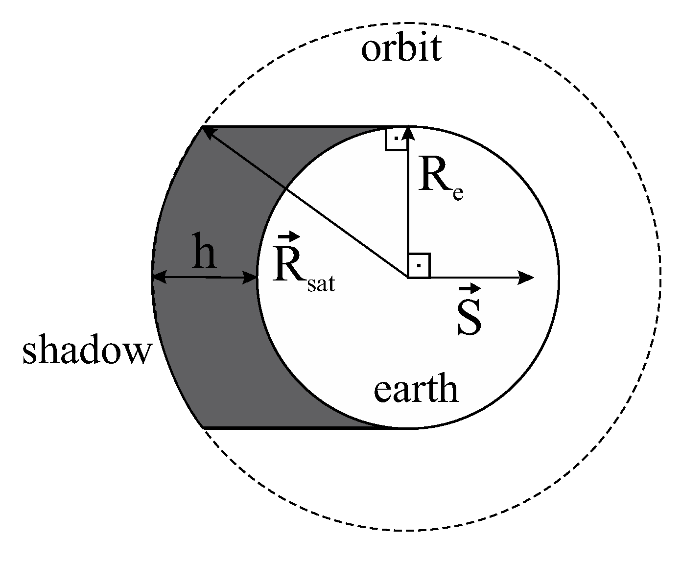
To estimate the view factor $F_{w\to e}\left(t\right)$, the Earth is idealized as a perfectly spherical emitter, much bigger than the satellite’s dimensions [28]. Therefore, it depends on the satellite and Earth’s distance, and so do the angles between each satellite and the Earth’s surface. Figure 4 illustrates these parameters.

The angle $\varphi$ between the satellite’s position and the Earth’s border is:

$$\varphi =sin(1/H)$$

(24)

The angle ${\gamma }_w$ between the orientation of surface w and the center of the Earth is given by Equation (25), and Equation (26) is the expression for the view factor [28].

$${\gamma }_w={cos}^{-1}\left(\frac{{\overrightarrow{n}}_w.{\overrightarrow{R}}_{\mathrm{sat}}}{\left|{\overrightarrow{n}}_w\right|\left|{\overrightarrow{R}}_{\mathrm{sat}}\right|}\right)$$

(25)

$$F_{w\to e}=\left\{\begin{array}{cc}\frac{cos\left({\gamma }_w\right)}{H^2},\hfill & {\gamma }_w\le \frac{\pi }{2}-\varphi \hfill \\ \frac{2}{\pi }\left(\frac{\pi }{4}-W_1+W_2\right),\hfill & \frac{2}{\pi }-\varphi \le {\gamma }_w\le \frac{2}{\pi }+\varphi \hfill \\ 0,\hfill & \mathrm{otherwise}\hfill \end{array}\right.$$

(26)

The terms in Equation (26) are:

$$W_1=\frac{1}{2}\left[{sin}^{-1}\left(\frac{\sqrt{H^2-1}}{Hsin\left({\gamma }_w\right)}\right)\right]$$

(27)

$$W_2=\frac{1}{2H^2}\left[cos\left({\gamma }_w\right){cos}^{-1}\left[-\sqrt{H^2-1}cot\left({\gamma }_w\right)\right]-\sqrt{H^2-1}\sqrt{1-H^2{\left[cos\left({\gamma }_w\right)\right]}^2}\right]$$

(28)

Infrared radiation: this source of thermal energy has its origin on Earth, which is always above absolute zero, and for this reason, emits radiation as:

$$Q_{{\mathrm{IR}}_w}\left(t\right)={\alpha }_w{A}_{r_w}{F}_{w\to e}\left(t\right)Q_e^{\prime \prime },$$

(29)

where $Q_e^{\prime \prime }$ is the radiative heat flux emitted by the Earth, at the infrared wave-length.

Satellite emission: the satellite’s emission of radiation to outer space, in the infrared spectrum, is governed by:

$$Q_{{\mathrm{sat}}_w\to \mathrm{spa}}\left(t\right)={\epsilon }_w{A}_{r_w}\sigma \left(T_w^4\left(t\right)-T_{\infty }^4\right),$$

(30)

where ${\epsilon }_w$ is the emissivity of the surface in the infrared spectrum, $\sigma$ is the Stefan-Boltzmann constant ($5.67\times {10}^{-8}$ W/m${}^2$K${}^4$), $T_w$ is the temperature of PV w and $T_{\infty }$ is the temperature of space.

The parameters used in this work for the irradiance model are summarized in

Table 1. Parameters of the irradiance model.

Parameter	Value
$Q_{Sun}^{\prime \prime }$	1360 [W/m${}^2$]
$Q_e^{\prime \prime }$	237 [W/m${}^2$]
${\alpha }_w$	0.3 [-]
${\epsilon }_w$	0.3 [-]
$A_{r_w}$	0.01 m${}^2$
a	0.3 [-]
$T_{\infty }$	2.7 K

.

The solar irradiance is constant and equal to 1360 W/m${}^2$ in this model, as shown in Table 1. In reality, this parameter changes primarily with the Earth/Sun distance and the 11-year solar cycle. However, the impact of these variations are within the model’s uncertainties.

As observed in Equation (30), the boundary condition is a function of the temperature at photovoltaic panels ($T_w\left(t\right)$), a variable to be solved in the thermal model. More information on irradiance models can be found in [29].

2.4. Thermal Model

To simulate the heat transfer over the satellite, the classical energy balance is conducted along the CubeSat’s full orbit, which is an environment where radiation and conduction are the main processes of heat transfer. In this work, the lumped parameter approach will be adopted, then parts of the satellite will be represented by nodes whose temperature gradient inside each node is negligible. To account for temperature gradients among the nodes is used the finite difference method. Therefore, the energy equation in each part of the satellite is indicated in Equation (31) ($\forall w=1,\dots ,7$):

$$Q_{r_w}\left(t\right)+Q_{T_w}\left(t\right)+Q_{{\mathrm{int}}_w}\left(t\right)=m_w{v}_w\frac{d{T}_w}{dt}\left(t\right)$$

(31)

The sub-index w represents the main parts, or a node of the CubeSat, and each node has mass equal to m, specific heat v, temperature T, thermal radiation rate $Q_r$, net heat transfer between internal parts $Q_T$, and internal heat generation $Q_{\mathrm{int}}$. Notice from previous section that $Q_{r_7}=0$. The system is solved by the Newton–Raphson method, and the time derivative in Equation (31) is discretized iteratively—by iterations “it”—at $it$ and $it-1$.

The net heat transfer between internal parts occurs by conduction and radiation processes. To keep the model simple, this term will be given by Equation (32), where $R_{T_w}$ is a thermal resistance of node w.

$$Q_{T_w}\left(t\right)=\left\{\begin{array}{cc}\frac{T_7\left(t\right)-T_w\left(t\right)}{R_{T_w}}\hfill & \mathrm{if}w\le 6\hfill \\ {\displaystyle \sum _{w=1}^6}\frac{T_w\left(t\right)-T_7\left(t\right)}{R_{T_w}}\hfill & \mathrm{if}w=7\hfill \end{array}\right.$$

(32)

The internal heat generation $Q_{\mathrm{int}}\left(t\right)$ is non-zero only for the battery node, where an electrical heater with power $P_H\left(t\right)$ is introduced, ruled by Equation (33).

$$Q_{{\mathrm{int}}_w}\left(t\right)=\left\{\begin{array}{cc}0\hfill & \mathrm{if}w\le 6\hfill \\ P_H\left(t\right)\hfill & \mathrm{if}w=7\hfill \end{array}\right.$$

(33)

The remaining parameters used in the thermal model are summarized in

Table 2. Parameters of the thermal model.

Parameter	Value
$R_{T_{w=1,\dots ,7}}$	100 K/W
$m_{w=1,\dots ,6}$	0.05 kg
$v_{w=1,\dots ,6}$	1000 J/(kg K)
$m_{w=7}$	0.06 kg
$v_{w=7}$	800 J/(kg K)

. Except for the arbitrary value for $R_{T_w}$, these values are approximations of numbers found in the literature—for example, in [19,30,31].

2.5. Heater Analysis

The heater in this work is a pure resistive load, so every power ($P_H\left(t\right)$) produced on it is transformed into heat, given by:

$$P_H\left(t\right)=\frac{{\left(V_B\left(t\right)D\left(t\right)\right)}^2}{R_H},$$

(34)

where $V_B\left(t\right)$ is the battery’s voltage, $D\left(t\right)$ is the duty cycle of a PWM (Pulse-width modulation) signal and $R_H$ is the electrical resistance of the heater. Thus, by assuming the thermal resistance to be equal to $R_T$ for every node of the satellite, as shown in Table 2, and applying the Laplace transform to Equation (31), the temperature at the battery ($T_7$) can be calculated by:

$$T_7\left(s\right)=\frac{P_H+\frac{1}{R_T}{\displaystyle \sum _{w=1}^6}{T}_w}{m_7{v}_{7}s+\frac{6}{R_T}}$$

(35)

Notice that the $T_7\left(s\right)$ has a time constant given by

$$\tau =\frac{m_7{v}_7{R}_T}{6},$$

(36)

showing that the settling time of the battery temperature is proportional to its mass, specific heat and to the thermal resistance. Additionally, Equation (35) can be used to estimate $T_7\left(t\right)$ by means of an Inverse Laplace transform, as

$$T_7\left(t\right)=\frac{R_T}{6}\left(P_H+\frac{1}{R_T}\sum _{w=1}^6{T}_w-exp\left(-\frac{6t}{R_T{m}_7{v}_7}\right)\right)$$

(37)

Given a certain D value, the steady-state value of $T_7$ is obtained by Equation (38).

$$T_7(\infty )=\frac{R_T}{6}\left(\frac{{\left(V_{B}D\right)}^2}{R_H}+\frac{1}{R_T}\sum _{w=1}^6{T}_w\right)$$

(38)

The duty cycle D can be isolated from Equation (38):

$$D=\sqrt{\left(T_7(\infty )\frac{6}{R_T}-\frac{1}{R_T}\sum _{w=1}^6{T}_w\right)\frac{R_H}{V_B^2}}=\sqrt{\left(\sum _{w=1}^6\frac{T_7(\infty )-T_w}{R_{T_w}}\right)\frac{R_H}{V_B^2}}=\sqrt{\frac{Q_{T_w}}{P_{H_{max}}}}$$

(39)

From Equation (39) it can be concluded that the cyclical ratio necessary to maintain a certain desired battery temperature is a ratio between its heat exchange and the maximum power input given by the heater.

2.6. Electrical Model

Electrical power system (EPS) architectures can have control in the solar panels, although the so-called direct energy transfer (DET) cannot [23,32]. In these architectures, the solar panels’ voltage depends on the battery voltage, and this varies depending on the power budget. Therefore, heaters’ power consumption affects battery voltage and energy harvesting, impacting the satellite’s energy balance.

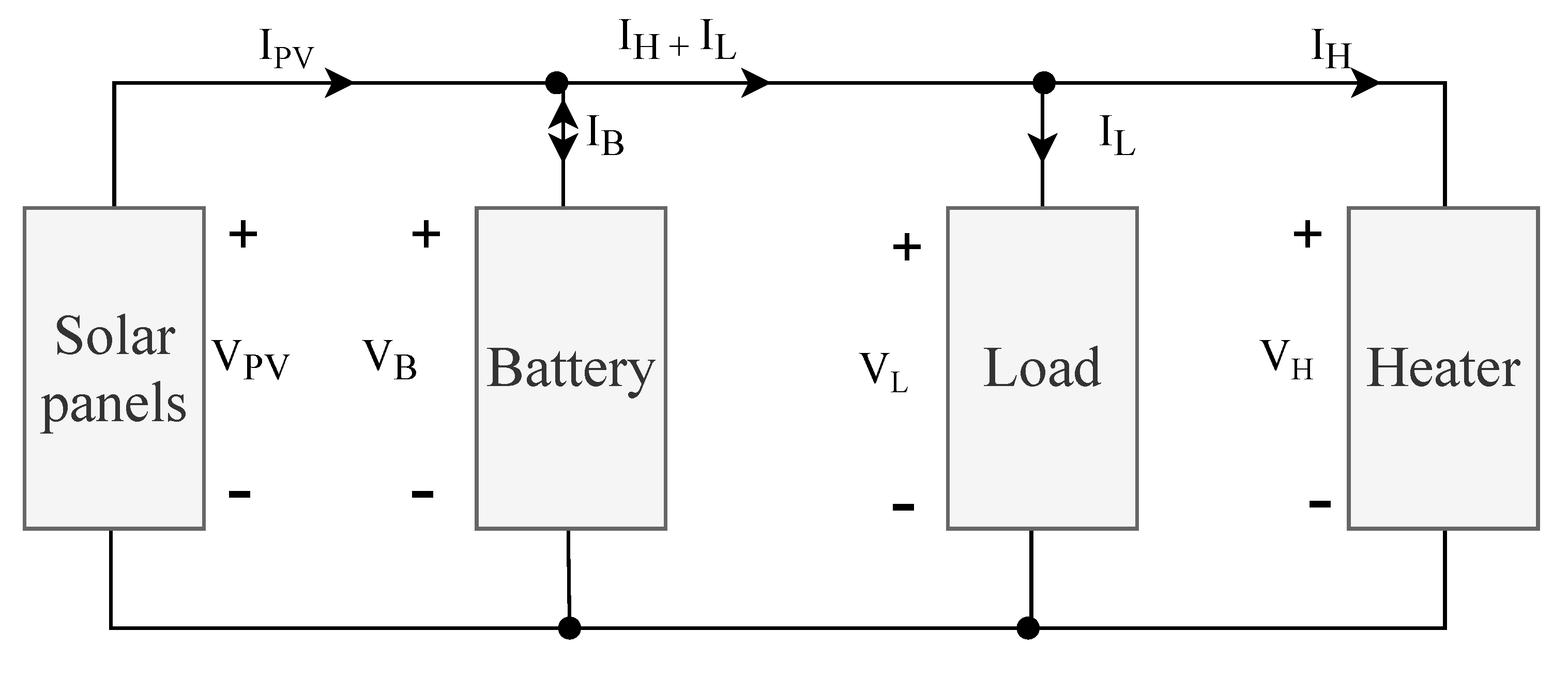
The directly coupled architecture is a DET topology, which is the simplest energy harvesting model [24]. Figure 5 shows a simplified directly coupled circuit diagram, where it has a single block representing solar panels. However, there are six solar panels, which are connected in parallel. This architecture requires that the solar panels, loads, and batteries have compatible voltage. As it was already exposed, the solar panels operate at almost the same voltage as the battery voltage, not always on their maximum power point. In this analysis, the passive components between the solar panels and the battery were not considered in the circuit. Figure 5 shows how to calculate the battery current $I_B$:

$$I_B\left(t\right)=I_H\left(t\right)+I_L\left(t\right)-\sum _{w=1}^6{I}_{{\mathrm{PV}}_w}\left(t\right)$$

(40)

$I_L$ is the load current, $I_H$ is the heater current, and $I_{\mathrm{PV}}$ is the photovoltaic panels’ current. The heater current will be expressed in Equation (41) with a resistance for the heater $R_H$ and a duty cycle D of a PWM signal control, already introduced in Section 2.5.

$$I_H\left(t\right)=\frac{V_B\left(t\right)D\left(t\right)}{R_H}$$

(41)

The load current $I_L$ depends on the load power $P_L$, defined as:

$$I_L\left(t\right)=\frac{P_L\left(L\right)}{V_B\left(t\right)}$$

(42)

The solar panel and battery models are required in the above expressions, and they will be evaluated in the following sections.

2.6.1. Solar Panel

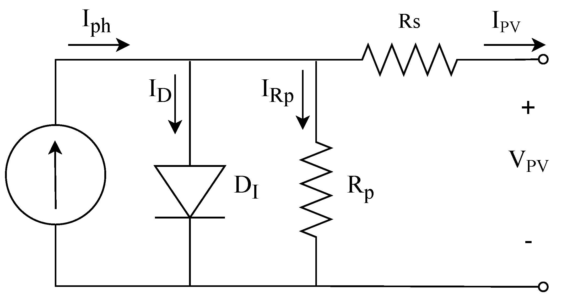
The solar panel is composed of several photovoltaic cells, which ideally can be modeled by a diode $\mathrm{DI}$ (PN junction) in parallel with a current source $I_{{\mathrm{ph}}_w}$ (photovoltaic effect) [12]. A practical model includes a bypass resistor $R_{p_w}$ with a series resistor $R_{s_w}$, the first one due to current leakage, spikes diffusion, or other effects. The second is the series resistance, mainly due to metal contacts with the semiconductor. Figure 6 shows the solar cell equivalent circuit, where $I_{{\mathrm{ph}}_w}$ is the photogenerated current, $I_{{\mathrm{DI}}_w}$ is the inverse saturation current of the diode, $I_{{R_p}_w}$ is the parallel resistor current, $I_{{\mathrm{PV}}_w}$ is the solar cell current, and $V_{{\mathrm{PV}}_w}$ is solar cell voltage. As mentioned previously, in this EPS model $V_{{\mathrm{PV}}_w}$ is the battery voltage $V_B$.

The current $I_{{\mathrm{PV}}_w}$ for a panel w is defined with the following equation:

$$I_{{\mathrm{PV}}_w}\left(t\right)=I_{{\mathrm{ph}}_w}\left(t\right)-I_{{\mathrm{DI}}_w}\left(t\right)-I_{{R_p}_w}\left(t\right)$$

(43)

$I_{{\mathrm{ph}}_w}$ can be obtained from the solar panel short circuit current $I_{{\mathrm{sc}}_w}$, for a given solar irradiance $Q_{s_w}^{\prime \prime }$ (given by Equation (19)), and solar cell temperature $T_w$ obtained with the proposed thermal model. $I_{{\mathrm{ph}}_w}$ for a panel w is described as:

$$I_{{\mathrm{ph}}_w}\left(t\right)=I_{{\mathrm{sc}}_w}\frac{Q_{s_w}^{\prime \prime }\left(t\right)}{Q_{s_{w_0}}^{\prime \prime }}[1+\Delta I_{{\mathrm{sc}}_w}(T_w\left(t\right)-T_{w_0})],$$

(44)

where $Q_{s_{w_0}}^{\prime \prime }$ is the solar irradiance and $T_{w_0}$ the temperature for which $I_{{\mathrm{sc}}_w}$ has been obtained, $\Delta I_{{\mathrm{sc}}_w}$ is the coefficient that expresses the $I_{{\mathrm{sc}}_w}$ variation with temperature. These parameters are usually obtained from the solar cell datasheet.

The diode current is expressed by Equation (45) [24], where $I_{S_w}$ is the saturation current, ${\eta }_w$ is the ideality factor of the diode, k being the Boltzmann constant and q the charge of the electron.

$$I_{{\mathrm{DI}}_w}\left(t\right)=I_{S_w}exp\left(\frac{-q(V_B\left(t\right)+I_{{\mathrm{PV}}_w}\left(t\right)R_{s_w})}{{\eta }_{w}k{T}_w\left(t\right)}-1\right)$$

(45)

The saturation current of the diodes $I_{S_w}$ in calculated by Equation (46), where $V_q$ is the voltage of the Crystaline Silicon.

$$I_{S_w}\left(t\right)=I_{S{0}_w}{\frac{T_w\left(t\right)}{T_{w_0}}}^{\frac{3}{{\eta }_w}}exp\frac{q{V}_q}{{\eta }_{w}k(\frac{1}{T_w\left(t\right)}-\frac{1}{T_{w_0}})},$$

(46)

where $I_{S{0}_w}$ is calculated using the open-circuit voltage $V_{O{C}_w}$ and short circuit current $I_{S{C}_w}$ of the solar panel at the temperature $T_{w_0}$ (47).

$$I_{S{0}_w}=\frac{I_{S{C}_w}\left(T_{w_0}\right)}{exp\frac{q{V}_{O{C}_w}\left(T_{w_0}\right)}{{\eta }_{w}k{T}_{w_0}}-1}$$

(47)

Combining Equations (44), and (45) with Equation (43), the solar cell current is described in terms of circuit parameters, as shown in Equation (48).

$$\begin{array}{l}{I}_{{\mathrm{PV}}_w}\left(t\right)=I_{{\mathrm{sc}}_w}\frac{Q_{s_w}^{\prime \prime }\left(t\right)}{Q_{s_{w_0}}^{\prime \prime }}[1+\Delta I_{{\mathrm{sc}}_w}(T_w\left(t\right)-T_{w_0})]\\ \hspace{1em}\hspace{1em}\hspace{1em}\hspace{1em}\hspace{1em}\hspace{1em}\hspace{1em}-I_{S_w}exp\left(\frac{-q(V_B\left(t\right)+I_{{\mathrm{PV}}_w}\left(t\right)R_{s_w})}{{\eta }_{w}k{T}_w\left(t\right)}-1\right)\\ \hspace{1em}\hspace{1em}\hspace{1em}\hspace{1em}\hspace{1em}\hspace{1em}\hspace{1em}\hspace{1em}\hspace{1em}\hspace{1em}\hspace{1em}\hspace{1em}\hspace{1em}\hspace{1em}\hspace{1em}\hspace{1em}\hspace{1em}\hspace{1em}-\frac{V_B\left(t\right)+I_{{\mathrm{PV}}_w}\left(t\right)R_{s_w}}{R_{p_w}}\end{array}$$

(48)

Notice that in order to solve (48) for $I_{{\mathrm{PV}}_w}\left(t\right)$, one can rely on iterative methods like Newthon–Raphson [33]. The data presented in

Table 3. Parameters of the solar panel model.

Parameter	Value
$\eta$	3.25 [-]
$V_q$	1.12 [eV]
$I_{\mathrm{sc}}$	0.41 [A]
$V_{\mathrm{oc}}$	2.564 [V]
$R_s$	0.2242 [$\Omega$]
$\Delta I_{\mathrm{sc}}$	0.07
$R_p$	∞ [$\Omega$]

are used in this paper for the solar panel model.

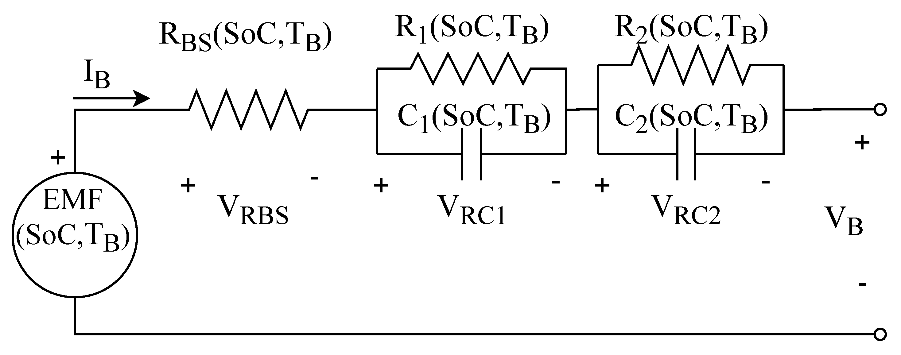
2.6.2. Battery

The battery model used in this paper assumes that the voltage of the battery is considered equal to the battery’s electromotive force $\mathrm{EMF}$, which is firmly related to $\mathrm{SoC}$ in series for an internal resistance $R_{\mathrm{BS}}$ and several resistor-capacitor blocks [7,34,35]. $R_{\mathrm{BS}}$ includes all the resistances between electrodes, current collectors, and electrolytes [34]. Those resistor-capacitor blocks represent the charge transfer and diffusion process [7]. Figure 7 shows the model used in this paper. Where the $R{C}_1$ block has a more considerable time constant, therefore, corresponds to the slowest response, on the contrary, the $R{C}_2$ block resembles a quick answer.

The battery state of charge $\mathrm{SoC}$ is calculated as:

$$\mathrm{SoC}\left(t\right)=\mathrm{SoC}\left(t_0\right)-\frac{1}{C_n}\underset{t_0}{\overset{t}{\int }}{I}_B\left(t\right)dt$$

(49)

where $\mathrm{SoC}\left(t_0\right)$ is the initial value of the $\mathrm{SoC}$, $C_n$ is the nominal capacity of the battery (in ampere-hours). $I_B\left(t\right)$ is the instantaneous current (positive for discharge and negative for charge). As discussed earlier, the $\mathrm{EMF}$ is heavily associated with $\mathrm{SoC}$. Analyzing the circuit of Figure 7 the battery voltage is defined by:

$$V_B\left(t\right)=\mathrm{EMF}\left(t\right)-R_{BS}\left(t\right)I_B\left(t\right)-V_{R{C}_1}\left(t\right)-V_{R{C}_2}\left(t\right),$$

(50)

where $R_{BS}\left(t\right)I_B\left(t\right)$ is the voltage drop across resistor $R_{\mathrm{BS}}$, $V_{R{C}_1}\left(t\right)$ and $V_{R{C}_2}\left(t\right)$ are the voltage drop across resistor-capacitor blocks $R{C}_1$ and $R{C}_2$ respectively, given by:

$$V_{R{C}_i}\left(t\right)=V_{R{C}_i}(t-\Delta t)+\frac{\Delta t}{C_i\left(t\right)}\left(I_B\left(t\right)-\frac{V_{R{C}_i}(t-\Delta t)}{R_i\left(t\right)}\right)$$

(51)

The values of internal parameters of the battery were approximated through look-up tables (LUTs), which were made through intermittent discharging experimental results [34] and are presented in the Appendix A.

3. Integrated Simulation Model

Considering the models introduced in the previous section, the proposed integrated model can be formulated as presented in Figure 8 in a flowchart. The problem is divided into the following main parts: orbit, attitude, irradiance, thermal, electrical, battery, and control model. To solve the satellite’s transient temperature field, the energy equation was implemented in the satellite’s main parts, here designed as the photovoltaic panels and battery, resulting in a total of seven equations. The irradiance in the boundary condition is transient to simulate different scenarios of spin and orbit.

The iterative process is performed until reaching the maximum desired simulation time. Overall, the simulation model consists of the following steps, contemplated in Figure 8.

• Given an initial SoC value, battery voltage, and temperature values, the algorithm calculates the CubeSat parameters for each iteration $it$;
• Given a time t, an iterative process takes place to calculate the new battery voltage;
• The heater power is calculated considering a possible controller;
• The load current is calculated based on the battery voltage and the maximum power drained (through tasks and/or payloads);
• The maximum current supplied by the solar panels is calculated based on the voltage of the battery, its temperatures and the irradiance affecting them;
• The battery parameters (SoC and current) are calculated based on the charging currents, heater and solar panels;
• The power balance is calculated based on the difference between the current supplied by the panels and that drained by the CubeSat (optional to be used in the control procedure, not necessary for the algorithm convergence);
• The battery voltage calculation is performed until convergence;
• A control procedure defined by the operator is performed, aiming to control the heater power and the allocated tasks;
• The calculation process is repeated for $t+\Delta t$.

4. Results

In this paper, the case study is based on the CubeSat 1U FloripaSat-I, whose orbit is nearly-circular and Sun-synchronous, and has an altitude of 620 km [36]. For these reasons, the orbit’s inclination is simplified to 90${}^{\circ }$ and perfectly circular. It is a condition that entails solar eclipse caused by the earth, so the unit vector inside $\left[M_i\right]$ is ${\overrightarrow{u}}_i=\left[0,1,0\right]$ and ${\theta }_i={90}^{\circ }$. The parameters to perform this inclination and the translation of the orbit’s satellite are summarized in

Table 4. Input for the orbit model.

${\mathit{\theta }}_{\mathit{i}}$	${\overrightarrow{\mathit{u}}}_{\mathit{i}}$	${\mathit{\theta }}_{\mathit{j}}$	${\overrightarrow{\mathit{u}}}_{\mathit{j}}$
90${}^{\circ }$	$\left[0,1,0\right]$	Equation (12)	$\left[0,0,1\right]$

.

It will be assumed that the orientation results from a passive attitude control based on magnets, which aligns the satellite with Earth’s magnetic field. Therefore, the matrix $\left[M_a\right]$ synchronizes one axis of the CubeSat with the Earth’s magnetic field, simplified as a dipole pattern. This axes is still free to rotate around itself, so a second matrix $\left[M_b\right]$ is used. The attitude scenario to be tested is summarized in

Table 5. Input for the attitude model.

${\mathit{\omega }}_{\mathit{a}}$ [Rot/Orbit]	${\overrightarrow{\mathit{u}}}_{\mathit{a}}$ (ERF)	${\mathit{\omega }}_{\mathit{b}}$ [Rot/Orbit]	${\overrightarrow{\mathit{u}}}_{\mathit{b}}$ (ORF)
2	$\left[1,0,0\right]$	10	$\left[0,0,1\right]$

. The CubeSat rotates twice per orbit around one axis to align with the Earth’s magnetic field, and the free spin around the secondary axis has the arbitrary value of 10 rotations/per orbit, representative of a spin condition without any damping.

We will also define the energy modes (L), in which the satellite will work, as presented in

Table 6. Operational mode of the satellite.

Mode: L	SoC [%]	${\mathit{P}}_{\mathit{L}}$ [W]
5	95–100	2.75
4	90–95	2.25
3	85–90	1.75
2	80–85	1.25
1	<80	0.25

. The energy levels are related to CubeSat’s maximum power consumption according to the battery’s state of charge. The energy levels presented, which are based on the CubeSat FloripaSat-1 [36], are related only to the available energy level ($\mathrm{SoC}$). However, they can be used, for example, to trigger energy-saving states, such as decreasing the energy usage in eclipse regions.

A simple control algorithm was employed to illustrate the case scenarios. The process defines the satellite’s maximum energy consumption according to the battery charge status and applies an on/off controller to the heater according to the defined temperature setpoint. To illustrate, a heater with $R_H=10$ $\Omega$ was used in the simulations. The timestep of the simulation was set to 1 s and the total time of the simulation was equivalent to 12 orbits.

4.1. Simulation Results

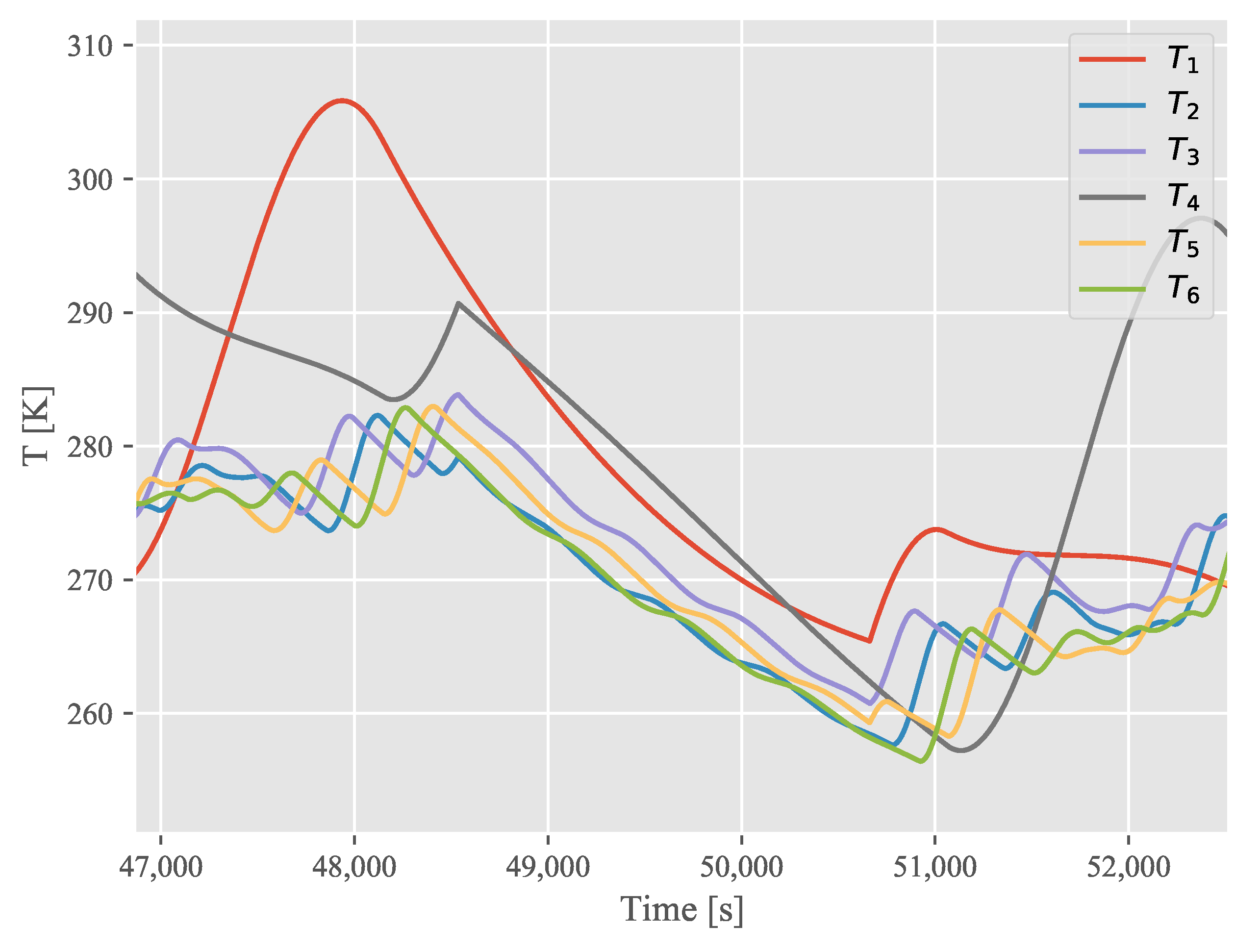
First, consider the temperature at the photovoltaic panels shown in Figure 9, which illustrates a scenario where no heater action is taken, that is, no temperature control. Sides 1 and 4 of the satellite become hotter because the attitude favors these surfaces towards the Sun. The decrease in the temperature in the middle of the figure results from the orbit’s period under the Earth’s shadow.

Figure 10 shows the power input ($P_{in}$) of the satellite concerning the variables battery voltage ($V_B$), average temperature of solar panels ($T_{PV}$) for each instant, and average solar irradiation ($Q_{ave}^{\prime \prime }$). All the parameters were normalized and valid for the portion of the orbit eclipse, and this behavior was captured for $T_{set}=273$ K. The integration of thermal-electrical parameters in this figure shows a temperature increase that should decrease the solar panels’ efficiency. However, this loss in efficiency is compensated by the increase in battery voltage due to the energy input, resulting in a closer behavior for the available irradiance and the power generation when the $V_B$ is higher.

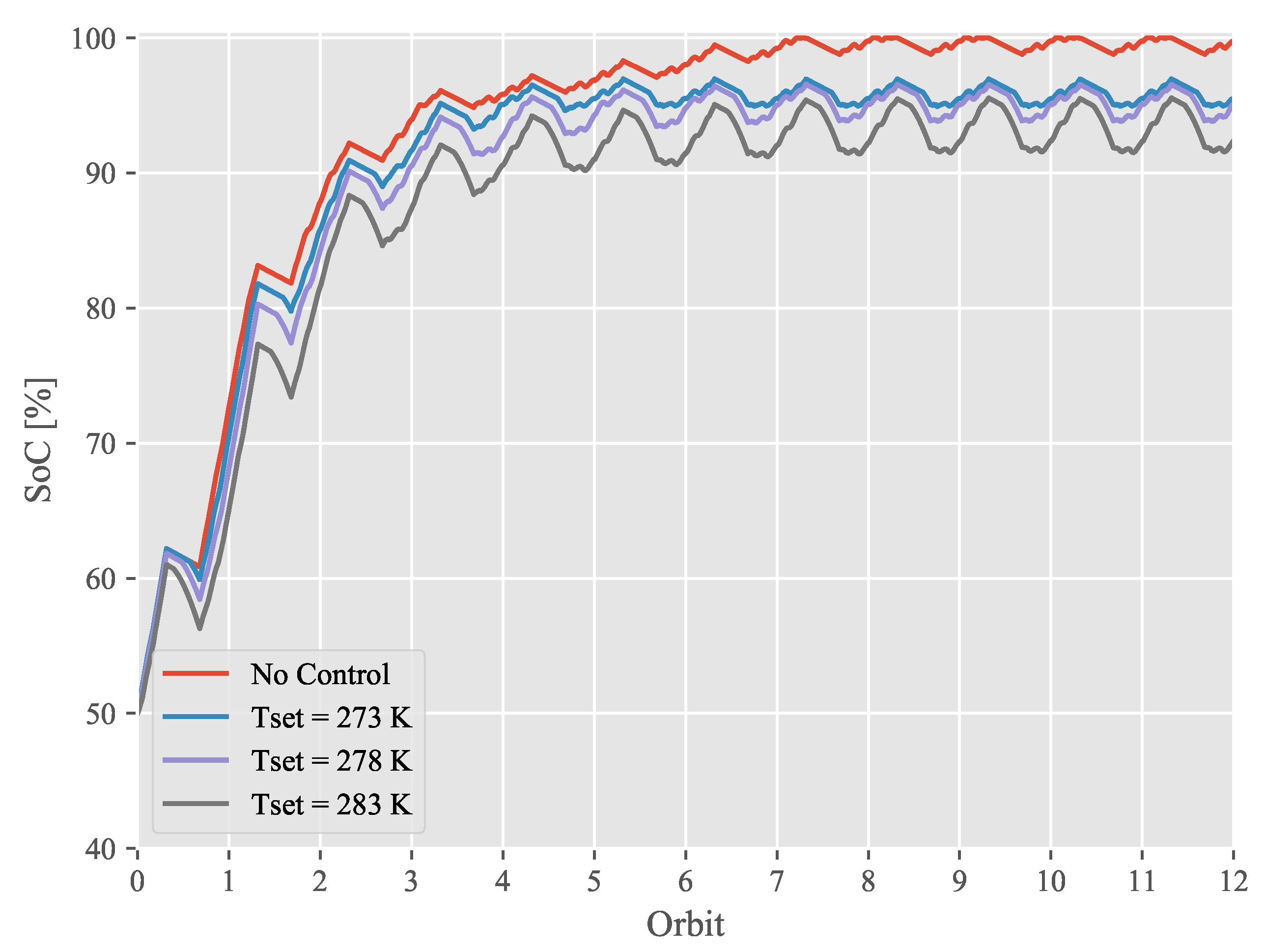
4.1.1. Fixed Temperature Setpoint

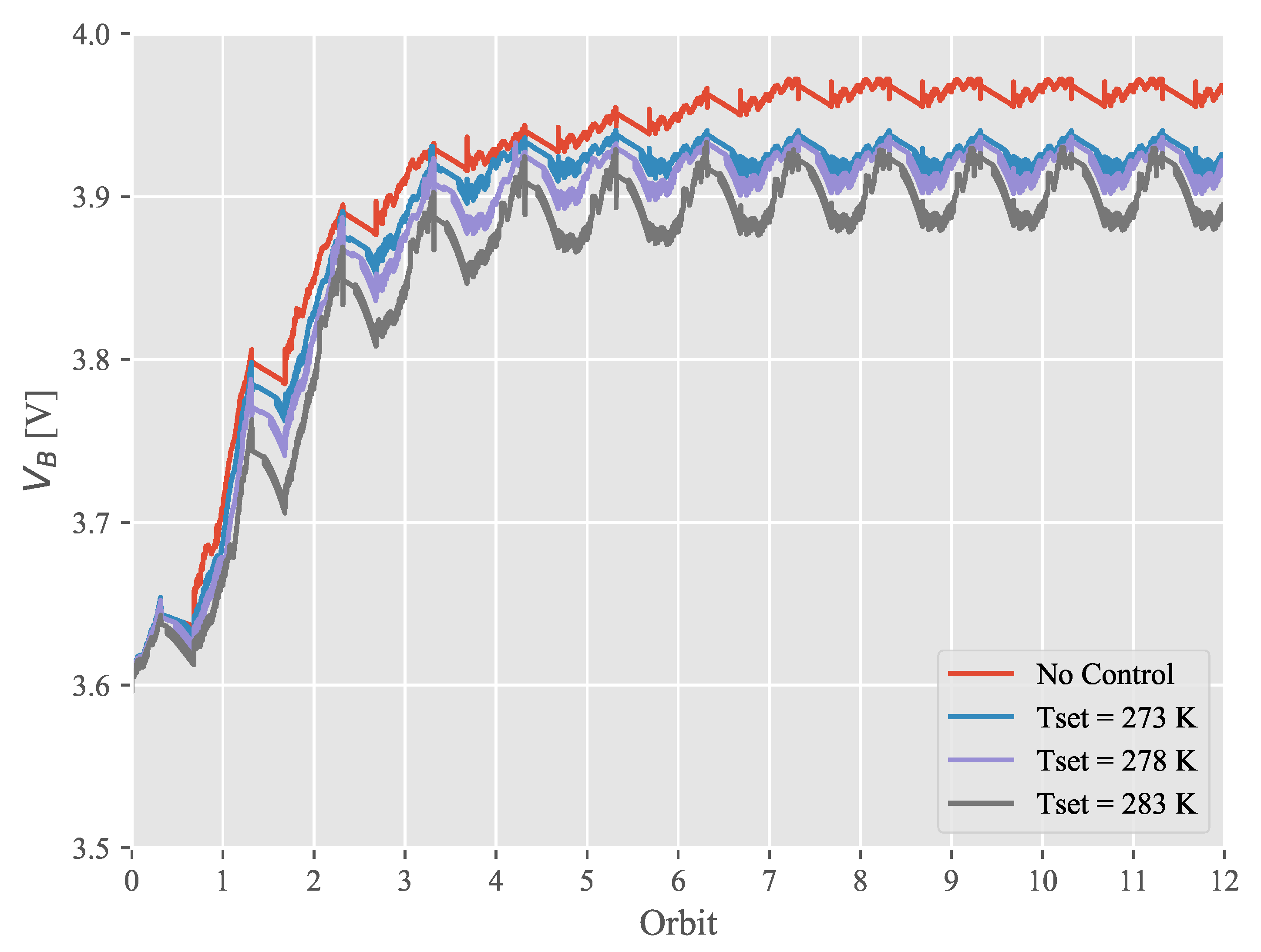
Under those considerations, initially, the behavior of the proposed model is illustrated under the following situations: no heater control, $T_{set}=273$ K, $T_{set}=278$ K, and $T_{set}=283$ K.

For the simulation process, we defined the initial SoC as $50\%$. The battery’s state of charge, voltage, and temperature, and the energy levels (L) are shown respectively in Figure 11, Figure 12, Figure 13 and Figure 14 for 12 cyclic orbits.

As can be seen, in the case with no heater (no control) in Figure 13, despite the CubeSat attaining the highest energy levels, the temperature reaches 265 K in eclipse regions, which tends to impact its lifespan and functioning. The most intensive use of the heater in the defined setpoints occurs in the eclipse regions. Typically in these regions, the satellite’s energy balance is negative, so tasks with high energy consumption should be avoided in those regions. As expected, a higher setpoint requires more energy from the system and keeps the satellite at lower energy levels (L) (Figure 14). In comparison, the cases with $T_{set}=273$ K, $T_{set}=278$ K and $T_{set}=283$ K have the heater on during the eclipse for 520, 916, and 1305 s, respectively.

For instance, consider the balance of energy shown in Figure 15, which zooms in on the satellite entering into an eclipse. Initially, the energy balance is close to 0 and constant as the heater is not activated, and CubeSat is in energy-saving mode $L=1$. However, as the battery’s temperature outside the eclipse was kept higher by the case with $T_{set}=283$ K, the activation of the heater suffers a delay, and its use is reduced when the satellite is within the eclipse. Maintaining a higher temperature outside the eclipse keeps the battery at a lower voltage and state levels as a negative point. Thus, a trade-off must be found between maintaining the battery temperature and its use.

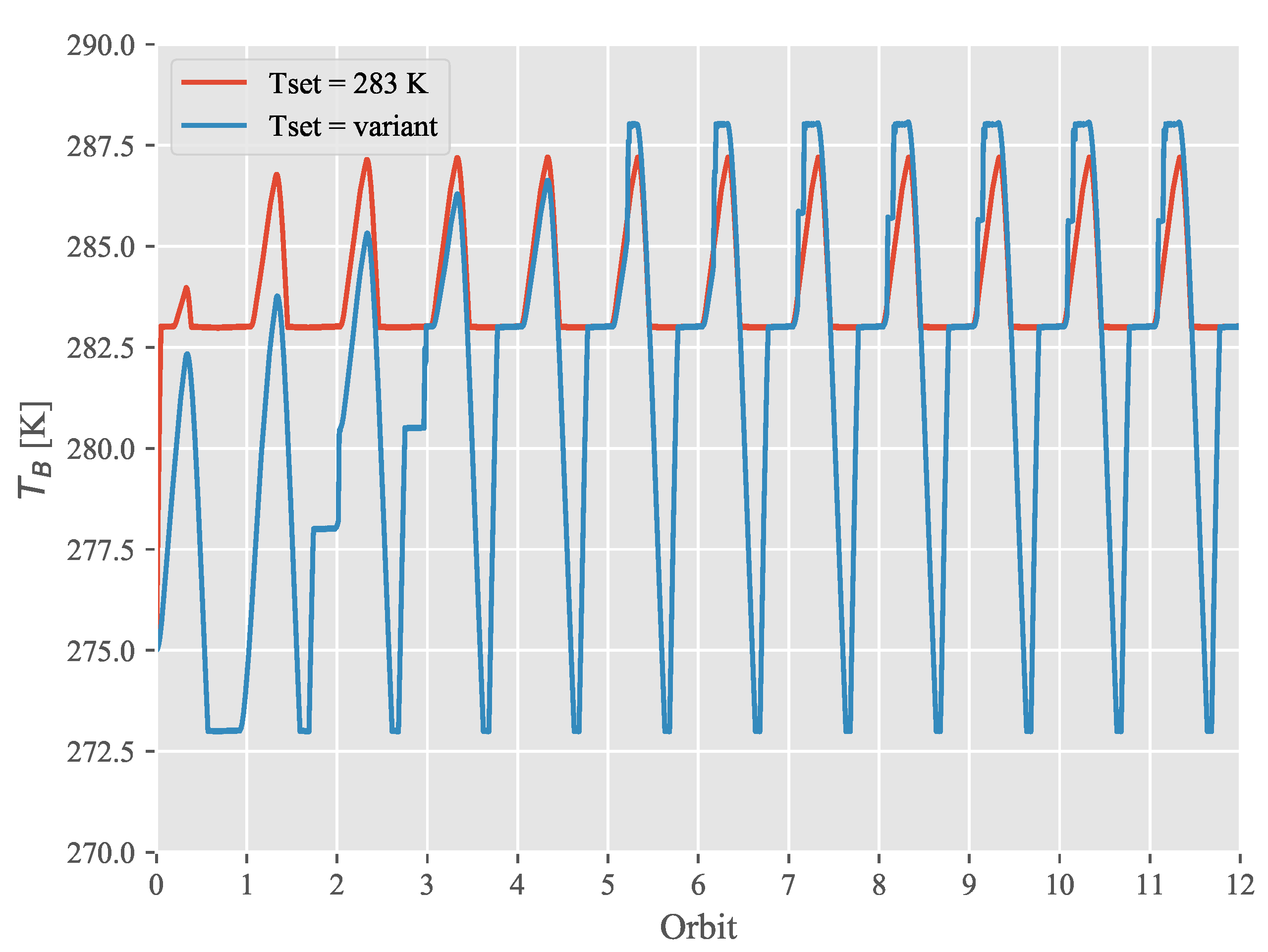
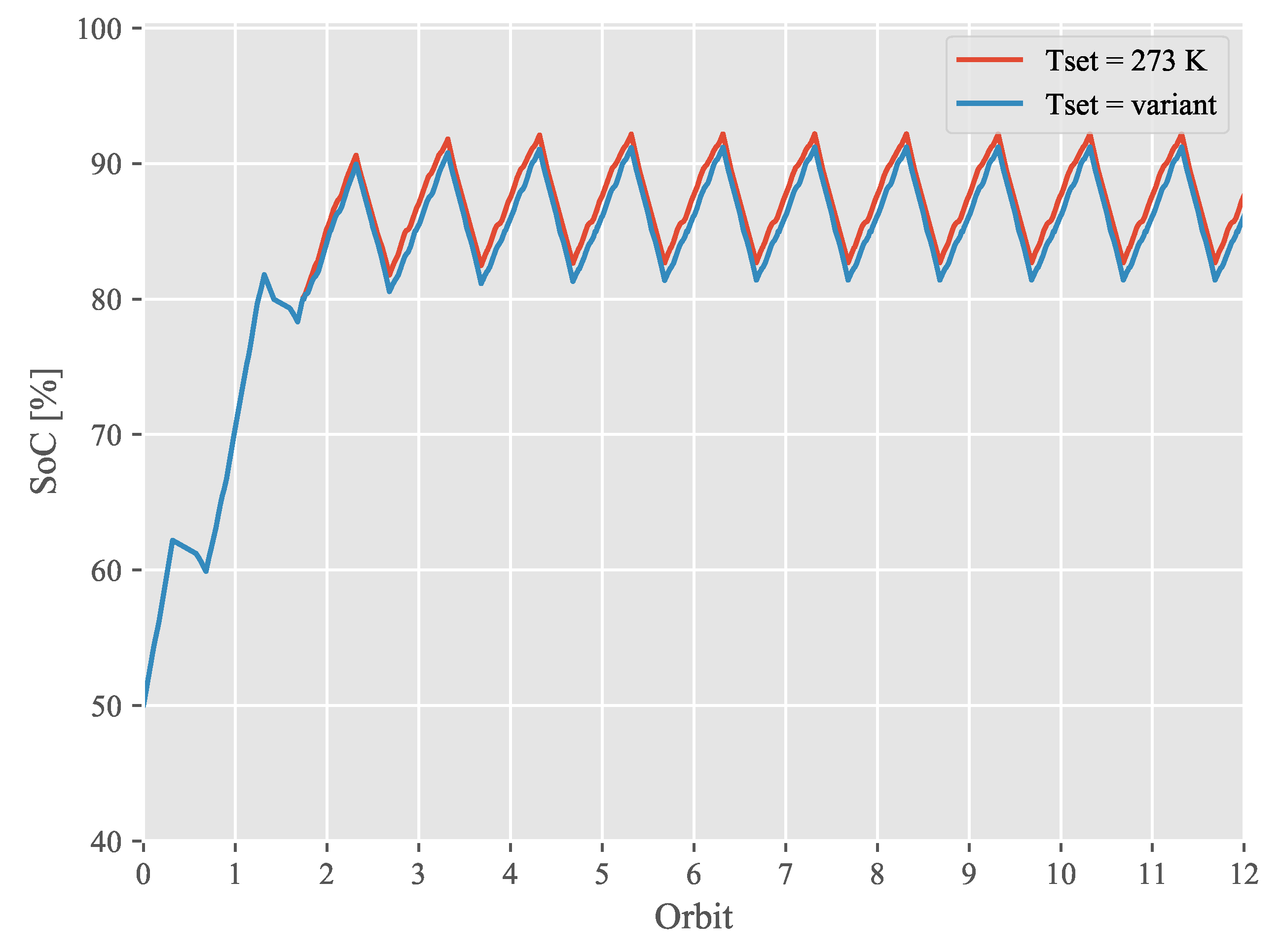
4.1.2. Variant Setpoints

The previous situation can be mitigated, for example, with the use of setpoints that vary according to the satellite’s energy level. Consider that for each energy level L, starting from 1 to 5, $T_{set}$ is now defined as follows: $T_{set}=[273,278,281,283,288]$. In other words, the setpoint will assume a different value depending on the level of energy available on the satellite. For example, if $L=1$ the setpoint will be 273 K, if $L=2$ the setpoint will be 278 K, and so on.

As can be seen in Figure 16, using different setpoints for different energy levels allows the battery’s state of charge to recover faster, and also maintain a higher $SoC$ during the orbit. This configuration results in the temperature behavior shown in Figure 17, in comparison with a constant $T_{set}=$ 283 K at the eclipse. The heater was kept on for 307 s during the variant case’s eclipse, the lowest value among all the simulated scenarios. Its high temperature explains this before the shadow and low setpoint during the eclipse.

4.1.3. No Energy-Saving Mode in an Eclipse

The previous cases considered that the CubeSat entered an energy-saving mode during the eclipse (that is, $L=1$). This subsection illustrates the same satellite behavior when no energy-saving actions are taken during the eclipse. For instance, Figure 18 and Figure 19 present, respectively, the state of charge and energy levels for scenarios without energy savings. Note that in this way, the variations in the state of charge of the battery tend to be greater, decreasing its useful life. Another consequence is that the higher expenditure during the eclipse state does not allow the CubeSat to return to the energy level $L=5$.

From the presented results, it is possible to perceive that the framework can be used to better understand the behavior of the temperature and energy of the satellite during the orbit. This allows designers to adapt their control algorithms according to the needs and power available in the target CubeSat.

4.1.4. MPPT

Another possibility brought by the integrated simulation method is the addition of an MPPT algorithm in the user-defined control phase. The MPPT algorithm is usually employed to search for the optimal point of the photovoltaic panel’s maximum power delivery. Figure 20 and Figure 21 illustrate one of the forms of MPPT known as “perturb and observe” in the integrated simulation model [37]. In this method, small disturbances in power consumed by the target device are used, and whether the power delivered by the panel has increased or decreased is analyzed. For more information on this method, please refer to [24].

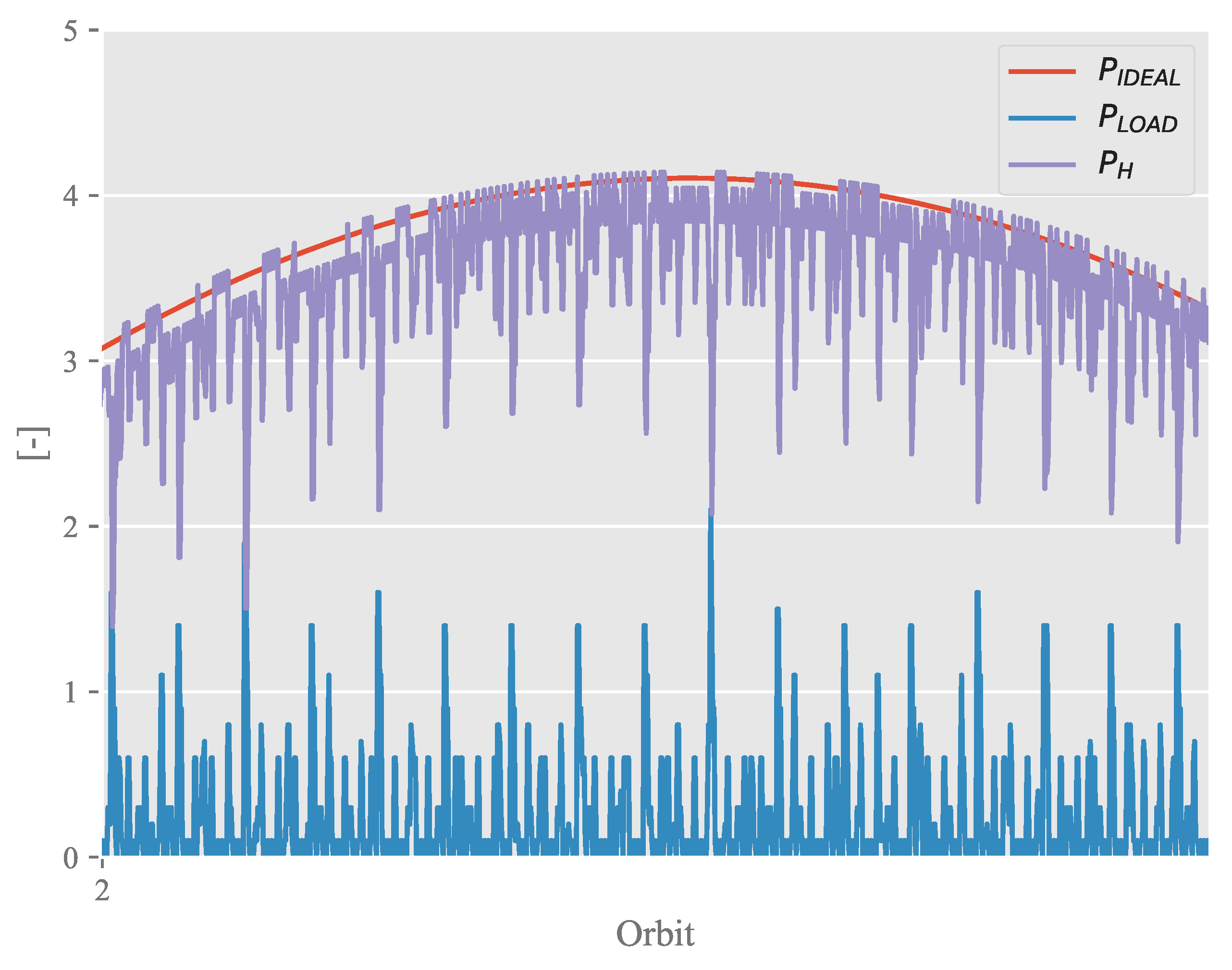
In Figure 20, the total input power of the satellite is compared with the ideal power that could be delivered for a given time. The control algorithm used selects the relevant tasks ($P_{\mathrm{LOAD}}$) in order to try to reach the maximum theoretical power. Note that over the period shown, the battery voltage increases, making use of the difference in excess power ($P_{\mathrm{TOTAL}}-P_{\mathrm{LOAD}}$). It is important to note that $P_{\mathrm{IDEAL}}$ is based on the ideal power that would be achieved by the best possible combinations of battery voltage and current—not necessarily using the instant battery voltage. This phenomenon causes the difference between $P_{\mathrm{TOTAL}}$ and $P_{\mathrm{IDEAL}}$.

Another interesting possibility in the use of MPPT is to take the surplus power of the execution of the tasks $P_{\mathrm{TOTAL}}-P_{\mathrm{LOAD}}$ to supply the heater, as illustrated in Figure 21 for a slice of an orbit. Notice that while trying to follow the maximum power, the system balances between the heater and the execution of tasks. In the illustrated scenario, when the sum of $P_H$ and $P_{\mathrm{LOAD}}$ exceeds the $P_{\mathrm{IDEAL}}$ line, it means that the battery is being used.

5. Conclusions

Given one of the CubeSats’ main challenges, which is proper energy management in a harsh environment, the platform’s limitations must be taken into account by the engineers during the satellite’s design. In this context, one of the challenges related to energy management is the need to keep the battery within acceptable temperature ranges, without wasting energy in the process.

To assist in this process, this paper proposes an integrated simulation model for the energy and temperature of CubeSats, taking into account aspects such as the electrical and thermal characteristics of the battery and the photovoltaic panels and their attitude dynamic in orbit.

Seven nodes idealize this integration of thermal and electrical models. While the model can support more nodes, such as different payloads, the heat transfer would still be limited to a simplified thermal resistance. Nevertheless, this simplification in the heat transfer by conduction and radiation among the main parts of the satellite is conducted at the expense of computational cost and simplicity for the user, a fundamental feature at the preliminary phases of development of a CubeSat, where the engineers may assess different configurations before proceeding into a much more complex model.

To illustrate the proposed model, a simulation scenario was generated for a 1U CubeSat in an orbit at 650 km with altitude and dynamics typical of CubeSats with passive attitude control. Tests were performed considering a heater with an on/off controller designed to keep the satellite temperature at an appropriate setpoint. The results presented the model’s capacity to report the battery’s thermal and electrical aspects, being able to help the designers with testing their own control system.

For future work, the search for a more accurate thermal model of solar panels is suggested, such as through the finite volumes method. The integrated model should be used for proposing new control systems and task-scheduling algorithms.