Several Cases for the Validation of Turbulence Models Implementation

Abstract

This paper presents several test cases that were used to validate the implementation of two turbulence models in the UNS3D code, an in-house code. The two turbulence models used were the Shear Stress Transport model and the Spalart–Allmaras model. These turbulence models were explored using the numerical results generated by three computational fluid dynamics codes: NASA’s FUN3D and CFL3D, and UNS3D. Four cases were considered: a flat plate case, an airfoil near-wake, a backward-facing step, and a turbine cascade known as the Eleventh Standard Configuration. The numerical results were compared among themselves and against experimental data.

1. Introduction

Computational fluid dynamics (CFD) has become an integral part of the design systems in aerospace and other engineering fields. The increase in computational power in the last two decades allows us to tackle complex, engineering relevant problems. Using today’s supercomputers, it has become customary to solve transport phenomena problems with tens or hundreds of millions of grid points and generate results overnight.

As the hardware improves, the models used for predicting transport phenomena should also improve. One standing challenge for flow simulation is the turbulence modeling. As direct numerical simulation is still too computationally expensive for engineering relevant flows, the governing mass, momentum, and energy equations must be closed using a turbulence model.

The widely used $\kappa -ϵ$ turbulence model developed by Jones and Launder [1] cannot properly capture the turbulent boundary layer up to flow separation. The first turbulence model that accurately predicted separated airfoil flows was the Johnson–King model [2]. Being an algebraic model, the Johnson–King model was not easily extensible to three-dimensional flow solvers. The $\kappa -\omega$ turbulence model proposed by Wilcox [3] improved the prediction for adverse pressure-gradient flows. In addition, the model has a simple formulation in the viscous sublayer. The $\kappa -\omega$ model, however, depends strongly on the freestream values of the specific turbulent dissipation rate, ${\omega }_f$. This issues was addressed by combining the $\kappa -\omega$ and $\kappa -ϵ$ models, so that the former models the inner region of the boundary layer and the latter models outer part. The resulting model, called the Shear Stress Transport turbulence model [4], was developed to respond to the need for accurate prediction of flows with strong adverse pressure gradients and separation. A turbulence model that is less computationally expensive than the Shear Stress Transport turbulence model is the Spalart–Allmaras model [5]. This is a one-equation model that models an eddy viscosity-like variable, $\tilde{\nu }$.

The purpose of this paper is to provide several cases that can be used to validate the implementation of the Shear Stress Transport and the Spalart–Allmaras turbulence models. The results generated using an in-house CFD code and two NASA codes, using a couple of turbulence models, are compared with experimental data.

The next section presents the physical model and provides details on the governing equations. This is followed by a brief summary of the numerical method used to solve the governing equations. The results section presents four validation cases, ranging from a flat plate to a cascade of turbine airfoils.

2. Physical Model

The governing equations used by the CFD solvers include of the mass, momentum, and energy conservation. These equations are supplemented by the equations used for modeling the turbulence effects. This section briefly presents the integral form of the mass, momentum, and energy conservation equations, as well as the turbulence models used in this work.

2.1. Mass, Momentum and Energy Conservation Equations

For an arbitrary finite volume, $\mathrm{\Omega }$, bounded by a closed surface, $\partial \mathrm{\Omega }$, a small surface, $dS$, with a unit normal vector, $\widehat{n}$, pointing outward from the control volume, the mass conservation equation is

$$\frac{\partial }{\partial t}{\int }_{\mathrm{\Omega }}\rho d\mathrm{\Omega }+{\oint }_{\partial \mathrm{\Omega }}\rho \left(\overrightarrow{v}·\widehat{n}\right)dS=0$$

(1)

where $\rho$ is the density and $\overrightarrow{v}$ is the velocity vector.

The momentum equation is

$$\frac{\partial }{\partial t}{\int }_{\mathrm{\Omega }}\rho \overrightarrow{v}d\mathrm{\Omega }+{\oint }_{d\mathrm{\Omega }}\rho \overrightarrow{v}\left(\overrightarrow{v}·\widehat{n}\right)dS=\oint \left(-p\mathbf{I}+\mathbf{\tau }\right)·\widehat{n}dS$$

(2)

where the scalar p is the pressure, $\mu$ is the dynamic viscosity coefficient, $\mathbf{I}$ is the identity tensor, and $\mathbf{\tau }$ is the viscous stress tensor.

The energy conservation equation for a calorically perfect gas is

$$\frac{\partial }{\partial t}{\int }_{\mathrm{\Omega }}\rho Ed\mathrm{\Omega }+{\oint }_{\partial \mathrm{\Omega }}\rho H\left(\overrightarrow{v}·\widehat{n}\right)dS={\oint }_{\partial \mathrm{\Omega }}k\left(\nabla T·\widehat{n}\right)+\left(\mathbf{\tau }·\overrightarrow{v}\right)\widehat{n}dS$$

(3)

where E is the total energy, H is the total enthalpy, T is temperature, and k is thermal conductivity.

2.2. Turbulence Models

Turbulence models are essential for producing accurate results when using Reynolds averaging. They provide the closure needed for the Reynolds-averaged Navier–Stokes (RANS) equations. The following sections describe the two turbulence models used in this work: the Shear Stress Transport (SST) turbulence model and the Spalart–Allmaras (S–A) turbulence model. Both turbulence models employ the Boussinesq eddy-viscosity hypothesis, where the Favre-averaged turbulent shear stresses, ${\mathbf{\tau }}^F$, is defined by

$${\mathbf{\tau }}_{ij}^F=2{\mu }_T{S}_{ij}-\left(\frac{2{\mu }_T}{3}\right)\frac{\partial {\tilde{v}}_k}{\partial x_k}{\delta }_{ij}-\frac{2}{3}\overline{\rho }\kappa {\delta }_{ij}.$$

(4)

where ${\mu }_T$ is the turbulent eddy viscosity, $S_{ij}$ is the strain rate tensor, $\kappa$ is the kinetic energy of the turbulent fluctuations, and ${\delta }_{ij}$ is the Kronecker delta.

2.2.1. Shear Stress Transport Turbulence Model

The Shear Stress Transport turbulence [4] model is a two-equation turbulence model that is a combination of a high Reynolds number $\kappa -ϵ$ turbulence model and the $\kappa -\omega$ turbulence model by Wilcox [6]. $\kappa$ denotes the kinetic energy of the turbulent fluctuations, $ϵ$ is the turbulence dissipation per unit mass, and $\omega$ is the root mean square fluctuating vorticity (or the rate of dissipation of energy in unit volume and time). The goal of combining the two models is to retain the best attributes of both models while fixing their weaknesses. For example, as the $\kappa -\omega$ model is sensitive to the freestream values of $\omega$, the Shear Stress Transport model switches to the $\kappa -ϵ$ model to resolve this issue. The Shear Stress Transport model is defined by the transport equations of the kinetic energy of the turbulent fluctuations, $\kappa$,

$$\begin{array}{cc}\hfill \frac{\partial \left(\rho \kappa \right)}{\partial t}+\frac{\partial \left(\rho v_j\kappa \right)}{\partial x_j}& =\frac{\partial }{\partial x_j}\left[({\mu }_L+{\sigma }_{\kappa }{\mu }_T)\frac{\partial \kappa }{\partial x_j}\right]+{\tau }_{ij}^F\begin{array}{c}\hfill \frac{\partial u_i}{\partial x_j}\end{array}-{\beta }^{*}\rho \omega \kappa \hfill \end{array}$$

(5)

and of the dissipation $\omega$,

$$\begin{array}{cc}\hfill \frac{\partial \left(\rho \omega \right)}{\partial t}+\frac{\partial \left(\rho v_j\omega \right)}{\partial x_j}& =\frac{\partial }{\partial x_j}\left[({\mu }_L+{\sigma }_{\omega }{\mu }_T)\frac{\partial \omega }{\partial x_j}\right]+{\tau }_{ij}^F\begin{array}{c}\hfill \frac{\partial u_i}{\partial x_j}\end{array}\frac{C_{\omega }\rho }{{\mu }_T}-\beta \rho {\omega }^2+\hfill \\ \hfill & +2(1-f_1)\frac{\rho {\sigma }_{{\omega }_2}}{\omega }\frac{\partial \kappa }{\partial x_j}\frac{\partial \omega }{\partial x_j}.\hfill \end{array}$$

(6)

$f_1$ is the blending function between the $\kappa -ϵ$ and the $\kappa -\omega$ turbulence models. This blending allows the Shear Stress Transport turbulence model to switch between the two turbulence models depending on (i) the distance from the wall and (ii) the region of the turbulent boundary layer is being analyzed. Variables ${\beta }^{*}$ and ${\sigma }_{\omega 2}$ are constant coefficients. Variables ${\sigma }_{\omega }$, ${\sigma }_{\kappa }$, $C_w$, and $\beta$ are non-constant coefficients that utilize the blending function, $f_1$ [4].

2.2.2. Spalart–Allmaras Turbulence Model

The Spalart–Allmaras turbulence model [5] is a one-equation turbulence model that solves the transport equation of an eddy viscosity-like variable, $\tilde{\nu }$,

$$\frac{D\tilde{\nu }}{Dt}=P-D+\frac{1}{\sigma }\left[\nabla ·(({\nu }_L+\tilde{\nu })\nabla \tilde{\nu })+c_{b2}{(\nabla \tilde{\nu })}^2\right]$$

(7)

where P and D are the production and destruction source terms,

$$\begin{array}{cc}\hfill P& =c_{b1}\left(1-f_{t2}\right)\tilde{S}\tilde{\nu }\hfill \end{array}$$

(8)

$$\begin{array}{cc}\hfill D& =\left(c_{w1}{f}_w-\frac{c_{b1}}{\begin{array}{c}\hfill {\kappa }_{SA}^2\end{array}}{f}_{v2}\right){\left[\frac{\tilde{\nu }}{d}\right]}^2\begin{array}{c}\hfill .\end{array}\hfill \end{array}$$

(9)

Constant coefficients include $\sigma$, $c_{b1}$, $c_{b2}$, $c_{w1}$, and ${\kappa }_{SA}$. The value d is the distance to the wall. Function $f_w$ is known as the wall function, as it is dependent on distance to wall, d. Viscous function $f_{v2}$ depends heavily on the ratio between the molecular kinematic viscosity, ${\nu }_L$, and the eddy-viscosity-like variable $\tilde{\nu }$. The modified vorticity term, $\tilde{S}$, is a function of the magnitude of vorticity, wall distance, and viscosities [5]. The Spalart–Allmaras turbulence model is a popular turbulence model for turbomachinery flows as it was designed for wall-bounded flows. As the Spalart–Allmaras turbulence model only solves for one equation, it is also inherently less computationally expensive than Shear Stress Transport.

The original turbulence model [5] has an additional trip term, $f_{t1}$, used to model transition to turbulence. Allmaras et al. [7] found that the two trip terms—$f_{t1}$ and $f_{t2}$—are unnecessary to simulate fully turbulent flows. The implementation used in this work does not use $f_{t1}$ [8]. In addition, the implementation is based on the compressible version that includes an update of the modified vorticity term [7].

3. Numerical Method

The turbulence models tested herein were implemented in three RANS solvers: CFL3D, FUN3D, and UNS3D. The first two flow solvers were developed by NASA. The third flow solver was developed at Texas A&M University. As detailed information is available for the NASA codes, this section focuses on presenting the numerical method used in the UNS3D code. UNS3D stands for Unstructured, Unsteady Three-Dimensional flow solver.

3.1. Spatial Discretization

The UNS3D flow solver uses a finite volume method for its spatial discretization. The UNS3D and the NASA’s FUN3D codes use a dual-mesh cell-vertex approach, while the NASA’s CFL3D code uses a cell-centered approach. The cell-vertex approach has better adaptability with mixed element grids. In addition, as for large grids the number of nodes is smaller than the number of elements, the cell-vertex method is computationally more efficient than the cell-centered method.

3.1.1. Convective Flux

UNS3D has several options for calculating the convective fluxes [9]. Herein, we selected an upwind scheme developed by Roe [10] with the additional entropy correction developed by Harten [11], known as the Roe’s flux-difference splitting scheme with the Harten entropy fix. The upwind scheme was chosen for its stability and ability to capture shock waves and boundary layers accurately.

3.1.2. Diffusive Flux

The diffusive flux describes flux of $\varphi$ entering the control volume $\mathrm{\Omega }$ due to the diffusion of $\varphi$. The diffusive flux is proportional to the gradient of $\varphi$ and is described as

$${\oint }_{\partial \mathrm{\Omega }}k\rho \left(\nabla \varphi ·\widehat{n}\right)dS$$

(10)

where k is a diffusivity coefficient, $\rho$ is the density, and $\nabla \varphi$ is the gradient of $\varphi$. As the gradients are stored at the nodes, a modified central scheme is used to calculate the edge-based gradients. An ordinary central scheme provides uncoupling between the local terms and the edge-based gradients. The following modification has been added to determine the edge-based gradients:

$$\nabla {\varphi }_{ij}=\frac{1}{2}\left(\nabla {\varphi }_i+\nabla {\varphi }_j\right)-\left[\frac{1}{2}\left(\nabla {\varphi }_i+\nabla {\varphi }_j\right)·{\widehat{e}}_{ij}\right]{\widehat{e}}_{ij}+\frac{{\varphi }_j-{\varphi }_i}{{\overrightarrow{x}}_j-{\overrightarrow{x}}_i}{\widehat{e}}_{ij}.$$

(11)

To calculate the diffusive flux, and for second-order spatial discretization, the gradients at the nodes must be calculated. As UNS3D is an unstructured and cell-vertex dual-mesh flow solver, there are specific numerical methods that can be used to calculate the gradients. The following gradient methods are available in UNS3D: Green-Gauss, least-squares, least squares with QR decomposition, and the Weighted Essentially Non-Oscillatory method. The results presented in this paper were generated using the Least Squares with QR decomposition as the primary gradient calculation method.

3.1.3. Second-Order Spatial Discretization

The state variables and their gradients, which are located at the nodes, are required to define a piecewise, linearly-varying approximation for a continuous flow field [12]. To achieve a linear variation, the nodal values across edge “$ij$” are reconstructed and defined as “left” and “right” state variables.

$$\begin{array}{c}\hfill {\overrightarrow{Q}}_L={\overrightarrow{Q}}_i+\frac{1}{2}{\mathrm{\Psi }}_i\left(\nabla {\overrightarrow{Q}}_i·\left({\overrightarrow{x}}_j-{\overrightarrow{x}}_i\right)\right)\\ \hfill {\overrightarrow{Q}}_R={\overrightarrow{Q}}_j-\frac{1}{2}{\mathrm{\Psi }}_j\left(\nabla {\overrightarrow{Q}}_j·\left({\overrightarrow{x}}_j-{\overrightarrow{x}}_i\right)\right)\end{array}$$

(12)

where $\mathrm{\Psi }$ is a limiter function. The limiter functions $\mathrm{\Psi }$ range from 0 to 1, and prevent non-physical oscillations and spurious solutions in the vicinity of large gradients. The solution limiters accomplish this by enforcing a monotonicity preserving scheme. The solution limiters used in this work were those proposed by Venkatakrishnan [13], Carpenter [14], and Dervieux [15].

3.2. Temporal Discretization

The terms of the Navier–Stokes equations can be grouped into spatial and temporal derivatives. The spatial derivatives consist of the source terms, and the convective and diffusive flux terms. These spatial derivative terms are grouped together to form the residual $\overrightarrow{R}$, thus the Navier–Stokes equations can be written as

$$\frac{\partial }{\partial t}{\overrightarrow{Q}}_i\left({\mathrm{\Omega }}_i\right)={\overrightarrow{R}}_i$$

(13)

where ${\overrightarrow{Q}}_i$ is the state vector, ${\mathrm{\Omega }}_i$ is the control volume, and ${\overrightarrow{R}}_i$ is the residual at node i.

The UNS3D solver can integrate (13) using either an explicit or implicit method. The results presented in this paper were obtained using only explicit time integration. Explicit time-integration utilizes either a first-order, forward finite difference approximation for the time derivative or a second-order scheme. The second-order time integration uses a four-stage Runge–Kutta method. Implicit residual smoothing is also available in the UNS3D solver. For unsteady simulations, UNS3D utilizes either single- or dual-time stepping.

3.3. Boundary Conditions

The implementation of boundary conditions can greatly affect the accuracy and convergence of the solution. The boundary conditions in the UNS3D solver have weak implementations. Weak implementation of boundary conditions refers to the scenario when the boundary conditions are not being directly applied to the nodal values, but instead to the boundary nodes created by the dual mesh. These boundary nodes are used in determining the fluxes from the boundary, and it is in these fluxes that the boundary conditions are satisfied.

3.3.1. Flow Boundary Conditions

For the subsonic inlet, the four conditions imposed from upstream infinity are the two components of the angle of attack, the total pressure, and the total temperature. The condition imposed from the interior of the domain is the outgoing Riemann invariant, $u+2c/(\gamma -1)$. For subsonic outlets, only one condition is imposed from downstream infinity, which is a user-specified static pressure. The conditions enforced from the interior of the domain are the entropy; tangential velocity; and the incoming and outgoing Riemann invariants, $u+2c/(\gamma -1)$ and $u-2c/(\gamma -1)$, respectively.

The wall boundaries are either inviscid and viscous wall boundaries. All wall boundaries enforce the no-penetration condition [16]. This is the only condition for inviscid walls. For viscous flows, the boundary conditions consist of the no-penetration and no-slip conditions [17], p. 80.

Symmetry boundary conditions are used to truncate the computational domain whenever there is a plane of symmetry. Symmetry boundary conditions are also used to simulate a two-dimensional (2D) flow field with a three-dimensional (3D) flow solver, creating what is known as a quasi-3D simulation. There are two conditions that must be satisfied with symmetry boundaries: no-penetration and the zero-gradient of state variables on the planes of symmetry. For this paper, a strong implementation of the zero-gradient condition was enforced, that is, both the boundary state vectors and state vectors on the symmetry boundary had the zero-gradient condition applied [18].

3.3.2. Shear Stress Transport Boundary Conditions

The Shear Stress Transport turbulence model primarily utilizes Neumann boundary conditions. The boundary conditions used are the recommended values from the original reference for the Shear Stress Transport turbulence model [4]. These boundary conditions are listed in Table 1.

Table 1. Shear Stress Transport boundary conditions (L-length of computational domain, $U_{\infty }$-velocity at upstream infinity).

Boundary	$\mathit{\kappa }$	$\mathit{\omega }$
Wall	$\kappa =0$	$\omega =10\frac{6\nu }{{\beta }_1{\left(\delta d_1\right)}^2}$
Freestream	$\frac{{10}^{-5}{U}_{\infty }^2}{R{e}_L}<\kappa <\frac{0.1U_{\infty }^2}{R{e}_L}$	$\frac{U_{\infty }}{L}<\omega <\frac{10U_{\infty }}{L}$
Inlet	$\frac{{10}^{-5}{U}_{\infty }^2}{R{e}_L}<\kappa <\frac{0.1U_{\infty }^2}{R{e}_L}$	$\frac{U_{\infty }}{L}<\omega <\frac{10U_{\infty }}{L}$
Symmetry	$\frac{\partial \kappa }{\partial n}$ = 0.0	$\frac{\partial \omega }{\partial n}$ = 0.0

The symmetry boundary condition for the Shear Stress Transport turbulence model follows the same structure as the governing equations, where the zero-gradient normal is applied for $\kappa$ and $\omega$. For the freestream and inlet boundaries, Dirichlet boundaries are enforced for a specific range. The freestream values of $\omega$ are obtained from turbulent intensities [4,19]. For the outlet, the values of $\kappa$ and $\omega$ are simply extrapolated. Periodic boundaries are applied to $\kappa$ and $\omega$ in the same manner as to the state vectors in the full-order model.

3.3.3. Spalart–Allmaras Boundary Conditions

The Spalart–Allmaras turbulence model utilizes both the Dirichlet and Neumann boundary conditions for its working variable $\tilde{\nu }$. Dirichlet boundary conditions are applied to the inlet/freestream and wall boundaries, while Neumann boundary conditions are applied for symmetry boundaries. Table 2 lists the boundary conditions for the Spalart–Allmaras turbulence model.

Table 2. Spalart–Allmaras boundary conditions.

Boundary	Dirichlet	Neumann
Wall	-	$\tilde{\nu }=0.0$
Freestream	-	$\frac{\tilde{\nu }}{{\nu }_L}=3-5$ (fully turbulent)
Inlet	-	$\frac{\tilde{\nu }}{{\nu }_L}=3-5$ (fully turbulent)
Symmetry	$\frac{\partial \tilde{\nu }}{\partial n}$ = 0.0	-

The symmetry boundary condition for the Spalart–Allmaras turbulence model follows the same structure as that of the governing equations, where the zero-gradient in the normal direction is applied for $\tilde{\nu }$. For the freestream and inlet boundaries, a $\tilde{\nu }/{\nu }_L$ value between 3 and 5 was used to simulate fully turbulent flows. For tripping the laminar-to-turbulent transition, $\tilde{\nu }/{\nu }_L$ must be less than 1. For the outlet, the value of $\tilde{\nu }$ is extrapolated. Periodic boundaries are applied to $\tilde{\nu }$ in the same manner as the state vectors in the mass, momentum, and energy conservation equations.

4. Results

The cases used for assessing the Spalart–Allmaras turbulence model follow the NASA’s turbulence modeling resource website [20]. There are two versions of the UNS3D code: a sequential version, UNS3D-SEQ, and a parallel version, UNS3D-PAR. Both the parallel and sequential versions of UNS3D implemented the Spalart–Allmaras turbulence model and underwent the same tests. The Shear Stress Transport turbulence model was also assessed using the same test cases. The results generated using UNS3D were compared against experimental data and numerical results obtained using FUN3D and CFL3D. The results of the sequential version of UNS3D used a coarser grid than that used by the parallel UNS3D and the NASA codes FUN3D and CFL3D.

4.1. Turbulent Flat Plate

The first case investigated was the turbulent flow over a flat plate. The turbulent flat plate case allowed one to validate the turbulence model against Coles’ Law of the Wake [21]. The velocity profile and distance from the wall were nondimensionalized to highlight the different regions of the turbulent boundary layer such as the log-region sublayer. Both the sequential and parallel versions of UNS3D were compared against the results from NASA’s FUN3D and CFL3D [20]. These results include dimensionless turbulent viscosity ${\mu }_T/{\mu }_{\infty }$, $\kappa$, and $\omega$ contours.

The computational domain and boundary conditions are illustrated in Figure 1. Two levels of mesh refinement were used for this case: where the parallel code used the finest grid and the sequential code used the third finest grid [20]. Figure 2 shows the coarse mesh. Table 3 specifies the freestream boundary conditions for the various turbulence models and codes. The freestream turbulence boundary conditions used in NASA’s FUN3D SST and CFL3D SST were above the recommended range [4], which is

$$\begin{array}{ccc}\hfill \frac{U_{\infty }}{L}<{\omega }_{\infty }<10\frac{U_{\infty }}{L}& \hfill & \hfill {10}^{-5}\frac{U_{\infty }^2}{R{e}_L}<{\kappa }_{\infty }<0.1\frac{U_{\infty }^2}{R{e}_L}.\end{array}$$

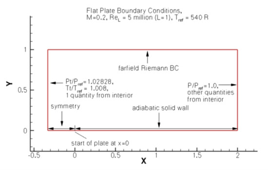
Figure 1. Flat plate boundary conditions [20].

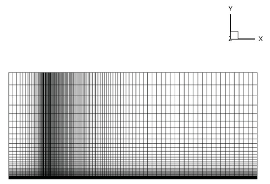
Figure 2. Flat plate coarse mesh.

Table 3. Turbulent Boundary Conditions for Flat Plate.

Code	Mesh	$\frac{{\tilde{\mathit{\nu }}}_{\mathit{\infty }}}{{\mathit{\nu }}_{\mathit{L}}}$	${\mathit{\omega }}_{\mathit{\infty }}\frac{{\mathit{\nu }}_{\mathit{L}}}{{\mathit{c}}_{\mathit{\infty }}^2}$	${\mathit{\kappa }}_{\mathit{\infty }}\frac{1}{{\mathit{c}}_{\mathit{\infty }}^2}$
UNS3D-SEQ SA	$2\times 137\times 97$	3.0	-	-
UNS3D-PAR SA	2 × 545 × 385	3.0	-	-
FUN3D SA	2 × 545 × 385	3.0	-	-
UNS3D-SEQ SST	2 × 137 × 97	-	$1\times {10}^{-6}$	$9\times {10}^{-9}$
UNS3D-PAR SST	2 × 545 × 385	-	$4\times {10}^{-8}$	$4\times {10}^{-10}$
FUN3D SST	2 × 545 × 385	-	$1\times {10}^{-6}$	$9\times {10}^{-9}$

The values used by NASA FUN3D correspond to

$$\begin{array}{ccc}\hfill {\omega }_{\infty }=125\frac{U_{\infty }}{L}& \hfill & \hfill {\kappa }_{\infty }=1.125\frac{U_{\infty }^2}{R{e}_L}.\end{array}$$

Therefore, FUN3D used turbulent freestream conditions that were approximately two orders of magnitude higher than the recommended range. UNS3D-PAR SST used values of $\kappa$ and $\omega$ that were in the recommended range:

$$\begin{array}{ccc}\hfill {\omega }_{\infty }=5\frac{U_{\infty }}{L}& \hfill & \hfill {\kappa }_{\infty }=0.05\frac{U_{\infty }^2}{R{e}_L}.\end{array}$$

We also generated UNS3D-PAR SST results using the turbulence boundary conditions used by the NASA codes. In this case, UNS3D-PAR SST produced $\kappa$ and $\omega$ contours that were approximately 10 percent smaller in magnitude than the NASA results. The results included in this paper for UNS3D-PAR SST used the turbulent boundary conditions in the recommended range, as stated in Table 3.

Figure 3 shows a comparison of the dimensionless turbulent viscosity predicted by the UNS3D-SEQ, UNS3D-PAR, and FUN3D codes using the Spalart–Allmaras turbulence model. A good agreement was obtained among the solutions of the three codes. A similar conclusion emerged by comparing the dimensionless turbulent viscosity predicted using the Shear Stress Transport turbulence model, shown in Figure 4. The large values of the turbulent viscosity extended farther away from the flat plate in the Spalart–Allmaras model compared to the Shear Stress Transport model, as observed by contrasting Figure 3 and Figure 4.

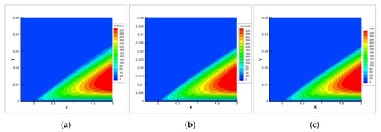
Figure 3. Contours of ${\mu }_T/{\mu }_{\infty }$ for flat plate using Spalart–Allmaras turbulence model: (a) UNS3D-SEQ, (b) UNS3D-PAR, and (c) FUN3D [20].

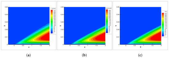
Figure 4. Contours of ${\mu }_T/{\mu }_{\infty }$ for flat plate using Shear Stress Transport turbulence‘model: (a) UNS3D-SEQ, (b) UNS3D-PAR, and (c) FUN3D [20].

Figure 5 shows the contours of the kinetic energy of the turbulent fluctuations, $\kappa$, produced by the Shear Stress Transport turbulence model. Similarly to the turbulent viscosity results, a good agreement is obtained among the solutions of the three codes.

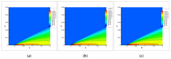
Figure 5. $k$ contours on flat plate using Shear Stress Transport turbulence model: (a) UNS3D-SEQ, (b) UNS3D-PAR, and (c) FUN3D [20].

Figure 6 shows that the main differences between the $\omega$ contours generated by UNS3D-PAR and FUN3D using the Shear Stress Transport model were located in the region near the inlet of the domain. FUN3D $\omega$ contours started at high values and dissipated as the flow went out of the domain. This difference was to be expected as the turbulent boundary conditions for FUN3D were at least one order of magnitude higher than those of the UNS3D-PAR. Overall, however, the UNS3D-PAR results were in good agreement with those of FUN3D in the region near the wall.

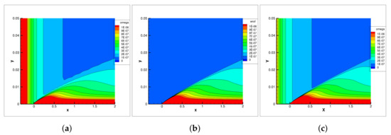
Figure 6. $\omega$ contours on flat plate using Shear Stress Transport turbulence model: (a) UNS3D-SEQ, (b) UNS3D-PAR, and (c) FUN3D [20].

Figure 7 shows the variation of dimensionless velocity $u^{+}=u/u^{*}$, where $u^{*}$ is the friction velocity, as a function of $y^{+}$. A good agreement is observed among the results generated by UNS3D-SEQ, UNS3D-PAR, and CFL3D codes, for both the Spalart–Allmaras and Shear Stress Transport models.

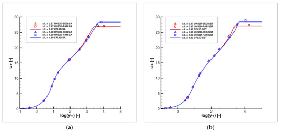
Figure 7. Law of the wake: (a) Spalart–Allmaras, and (b) Shear Stress Transport.

Figure 8 shows the skin friction coefficients predicted using the Spalart–Allmaras and Shear Stress Transport models. For the Spalart–Allmaras model, the skin friction coefficient was calculated using UNS3D-SEQ, UNS3D-PAR, and FUN3D codes. The agreement among the results generated by these three codes was excellent. For the Shear Stress Transport model, the skin friction coefficient was calculated using UNS3D-SEQ, UNS3D-PAR, and FUN3D codes. The skin friction coefficient predicted by the UNS3D-SEQ code was slightly smaller than the results predicted by the other two codes. Most likely, this difference is due to the fact that UNS3D-SEQ used a coarser grid than the other two codes, as shown in Table 3.

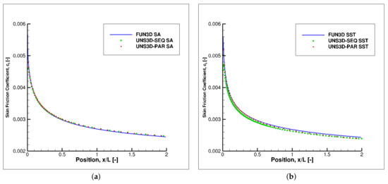
Figure 8. Skin friction coefficients for turbulent flat plate: (a) Spalart–Allmaras, and (b) Shear Stress Transport.

Figure 9 shows the predicted velocity profiles at two $x/L$ locations: 0.97 and 1.90. The results generated with the UNS3D-SEQ, UNS3D-PAR, and CFL3D codes agree well, for both the Spalart-Allmaras and the Shear Stress Transport models.

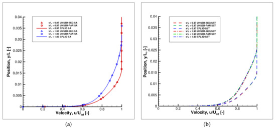
Figure 9. Velocity profiles on turbulent flat plate: (a) Spalart–Allmaras, and (b) Shear Stress Transport.

4.2. Two-Dimensional Airfoil Near-Wake

This test case is based off Model A airfoil, a convential airfoil that was experimentally investigated by Nakayama [22]. Model A airfoil is a 10%-thick conventional airfoil with a 61 cm chord. The angle of attack was 0 deg, the wind tunnel speed was 30 m/s, and the freestream turbulence level was 0.02%. The boundaries of the computational domain, shown in Figure 10, were 20 chords away from the airfoil. A detail of the mesh near the airfoil is shown in Figure 11. The input flow parameters used in the numerical simulation are listed in Table 4.

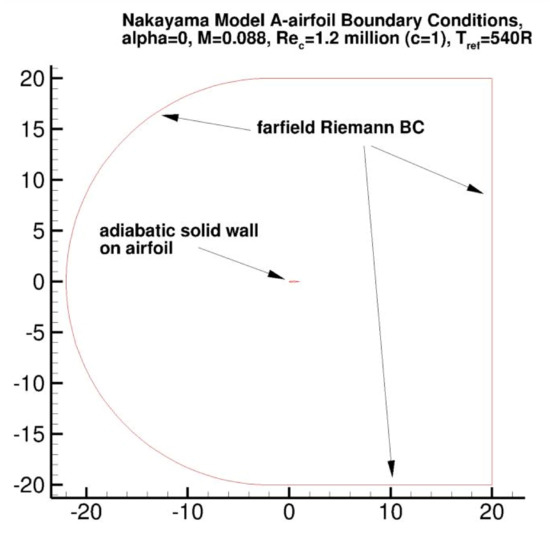
Figure 10. Airfoil boundary conditions [20].

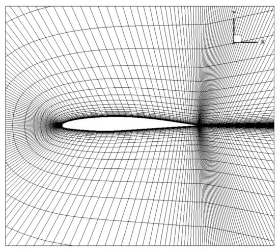
Figure 11. Detail of airfoil mesh.

Table 4. Input parameters for Nakayama airfoil.

${\mathit{p}}_{\mathbf{ref}}$	${\mathit{T}}_{\mathbf{ref}}$	${\mathit{M}}_{\mathbf{inlet}}$	Re	${\mathit{\mu }}_{\mathbf{ref}}$	$\frac{\tilde{\mathit{\nu }}}{\mathit{\nu }}$	${\mathit{\omega }}_{\mathit{\infty }}\frac{{\mathit{\nu }}_{\mathit{L}}}{{\mathit{c}}_{\mathit{\infty }}^2}$	${\mathit{\kappa }}_{\mathit{\infty }}\frac{1}{{\mathit{c}}_{\mathit{\infty }}^2}$
[Pa]	[K]	[-]	[-]	[Pa s]	[-]	[-]	[-]
62,000	300	0.088	1,200,000	1.838$\times {10}^{-5}$	3	4$\times {10}^{-8}$	4$\times {10}^{-10}$

As with the turbulent flat plate case, the freestream values of $\kappa$ and $\omega$ for UNS3D-PAR SST were different from the values used for the FUN3D simulation. Figure 12 shows the contour plots of the dimensionless turbulent viscosity ${\mu }_T/{\mu }_{\infty }$ at the airfoil’s trailing edge predicted using the Spalart–Allmaras model. There is good agreement between the results generated by the UNS3D-PAR and FUN3D codes. The turbulent viscosity predicted by the UNS3D-SEQ code, which used the coarse grid, was similar to the two codes; however, the lack of grid refinement at the trailing edge leads to a somewhat thicker wake.

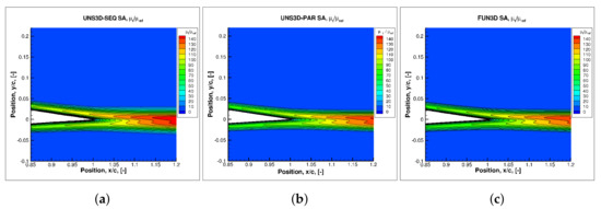
Figure 12. ${\mu }_t/{\mu }_{\infty }$ contours on Nakayama’s airfoil predicted with Spalart–Allmaras model: (a) UNS3D-SEQ, (b) UNS3D-PAR, and (c) FUN3D.

Figure 13 and Figure 14 show the contour plots of the turbulent kinetic energy, $\kappa$, and the specific dissipation rate, $\omega$, predicted using the Shear Stress Transport model. The agreement among the results generated by the three codes is good. While there are few differences on the turbulent kinetic energy contour plots, the specific dissipation rates are almost identical.

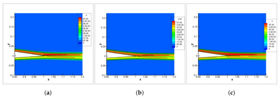
Figure 13. $k$ contours on Nakayama’s airfoil predicted with Shear Stress Transport model: (a) UNS3D-SEQ, (b) UNS3D-PAR, and (c) FUN3D.

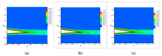
Figure 14. $\omega$ contours on Nakayama’s airfoil predicted with Shear Stress Transport model: (a) UNS3D-SEQ, (b) UNS3D-PAR, and (c) FUN3D.

Figure 15 compares the measured velocity profiles against the predicted ones at seven locations in the airfoil’s wake. These locations, measured from the airfoil leading edge, are: 1.01, 1.05, 1.20, 1.40, 1.80, 2.19, and 3.0 x/chord. The numerical predictions were done using the UNS3D-PAR code with the Spalart–Allmaras and the Shear Stress Transport models. The velocity profiles predicted using the Shear Stress Transport model matched the experimental data better than the Spalart–Allmaras model, although the Spalart–Allmaras model predicted the velocity profiles quite well.

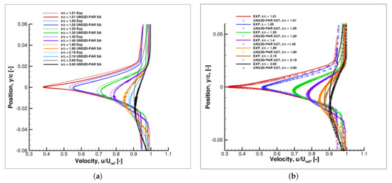
Figure 15. Velocity profiles on Nakayama’s airfoil: (a) Spalart–Allmaras, and (b) Shear Stress Transport.

Figure 16 compares the measured turbulent shear stresses $-\overline{u^{\prime }{v}^{\prime }}$ against the predicted ones at the same seven locations in the wake. Both the Spalart–Allmaras and Shear Stress Transport models were used in the UNS3D-PAR code. The two turbulence models predicted the general shape of the shear stresses, although there were some differences between the predicted results and the experimental data.

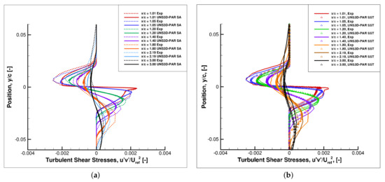
Figure 16. Dimensionless turbulent shear stress profiles on Nakayama’s airfoil: (a) Spalart–Allmaras, and (b) Shear Stress Transport.

4.3. Two-Dimensional Backward-Facing Step

The backward-facing step is a case proposed by Driver and Seegmiller [23] to test how well the turbulence model simulates separated flows. The backward-facing step case is a challenging problem as turbulence models generally have difficulty modeling separated flows.

The test configuration had a 100 cm long × 15.1 cm wide × 10.1 cm high rectangular inlet duct followed by a backward-facing step of H = 1.27 cm. The geometry of the computational domain of the backward-facing step, shown in Figure 17, is defined as a function of the step height, H. The experiment took place at atmospheric total pressure and temperature. The freestream velocity was 44.2 m/s. The Reynolds number based on step height was ${\mathrm{Re}}_H$ = 36,000. The boundary conditions are also shown in Figure 17. A detail of the mesh near the step is shown in Figure 18.

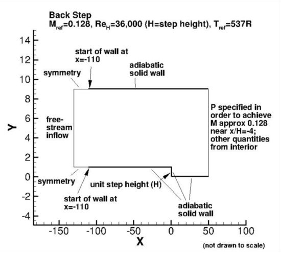
Figure 17. Backward-facing step geometry and boundary conditions [20].

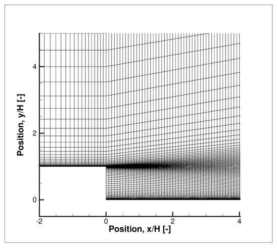
Figure 18. Detail of backward-facing step mesh.

Two grids were used for this test case: (1) the second coarsest and (2) the finest grid provided by the NASA Turbulence Modeling [20]. The results generated with the UNS3D-SEQ and UNS3D-PAR codes were compared against those generated with the NASA FUN3D and CFL3D codes which used the finest grid. The sets of results presented herein include velocity profiles, turbulent shear stresses, skin friction coefficients, and reattachment points.

Figure 19 compares the measured and predicted velocity profiles at four locations downstream from the step: $x/H$ = 1, 4, 6, and 10. The velocity profiles were calculated using the UNS3D-SEQ, UNS3D-PAR, and CFL3D codes with the Spalart–Allmaras and Shear Stress Transport models. There was a good agreement among the results of the three codes, for both turbulence models. The Shear Stress Transport model matched the experimental data better than the Spalart–Allmaras model near the step, at $x/H$ = 1. Away from the step, at $x/H$ = 4, 6, and 10, the Spalart–Allmaras model captured the velocity profiles better than the Shear Stress Transport model.

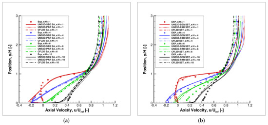
Figure 19. Velocity profiles on backward-facing step: (a) Spalart–Allmaras, and (b) Shear Stress Transport.

Figure 20 compares the measured and predicted friction coefficients. There is a relatively good agreement among the results produced by the UNS3D-SEQ, UNS3D-PAR, and CFL3D codes, using both Spalart–Allmaras and Shear Stress Transport models.

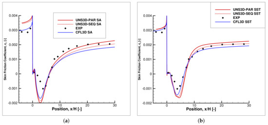
Figure 20. Coefficient of friction on backward-facing step: (a) Spalart–Allmaras, and (b) Shear Stress Transport.

The experimental investigation found the reattachment point to be at 6.26 ± 0.01 [23]. The predicted location of the reattachment point varied depending on the turbulence model. The Spalart–Allmaras model predicted an earlier reattachment, while the Shear Stress Transport model predicted a delayed reattachment. The predicted locations of reattachment point are summarized in Table 5.

Table 5. Location of reattachment point $x/H$ on backward-facing step.

	Spalart–Allmaras	Shear Stress Transport
CFL3D	6.07	6.35
FUN3D	6.10	6.50
UNS3D-SEQ	6.27	6.79
UNS3D-PAR	6.01	6.83

Figure 21 compares the measured and predicted turbulent shear stresses at four locations downstream from the step. The results predicted using the Shear Stress Transport model matched the turbulent shear stresses better than the Spalart–Allmaras model.

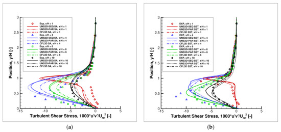
Figure 21. Dimensionless turbulent shear stress on backward-facing step: (a) Spalart–Allmaras, and (b) Shear Stress Transport.

4.4. Eleventh Standard Configuration

The Eleventh Standard Configuration contains two test cases from the experimental data obtained in the annular test cascade at EPF-Lausanne on a two-dimensional turbine cascade: (1) a subsonic, attached flow case, and (2) a transonic, separated flow case [24]. Herein, only the subsonic, attached flow case with stationary airfoils was simulated.

The airfoil chord is 77.8 mm, the pitch is 56.55 mm, and the stagger angle is −40.85$°$. The inflow angle is 15.2$°$. The input flow conditions are listed in Table 6.

Table 6. Input parameters for eleventh standard configuration, case 100.

${\mathit{p}}_{\mathbf{tot}}$	${\mathit{T}}_{\mathbf{tot}}$	${\mathbf{M}}_{\mathbf{inlet}}$	${\mathbf{Re}}_{\mathit{L}}$	${\mathit{\mu }}_{\mathbf{ref}}$	$\frac{\tilde{\mathit{\nu }}}{\mathit{\nu }}$	${\mathit{\omega }}_{\mathit{\infty }}\frac{{\mathit{\nu }}_{\mathit{L}}}{{\mathit{c}}_{\mathit{\infty }}^2}$	${\mathit{\kappa }}_{\mathit{\infty }}\frac{1}{{\mathit{c}}_{\mathit{\infty }}^2}$
[Pa]	[K]	[-]	[-]	[Pa s]	[-]	[-]	[-]
124,600	330	0.31	446,000	1.846$\times {10}^{-5}$	3	4$\times {10}^{-8}$	4$\times {10}^{-10}$

Figure 22 shows the computational mesh for two adjacent airfoils. The flow, however, was calculated over a single passage by using periodic boundary conditions to simulate the rest of the cascade. A multiblock O4H-grid padded with inlet and outlet H-grids was used to discretize the computational domain. The number of grid nodes varied between 39 k on the coarse mesh to 182 k on the fine mesh. Figure 22 shows the coarse grid. In the $x-y$ plane, the fine mesh used 401 × 101 nodes on the O-grid, 62 × 49 nodes on the block prior to the leading edge, 82 × 29 nodes on the block downstream from the trailing edge, 305 × 25 above and below the airfoil, 160 × 97 at inlet, and 200 × 77 at outlet. One cell was used the spanwise direction, as the flow was modeled as two-dimensional and the flow solver was three-dimensional.

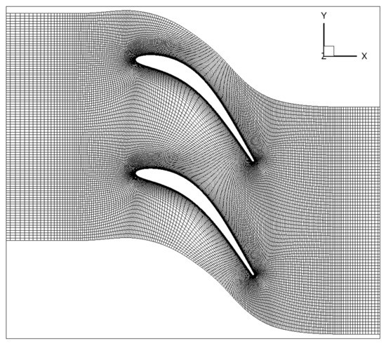
Figure 22. Eleventh standard configuration computational grid.

Figure 23 shows a comparison of the measured and predicted Mach number over the airfoil. The UNS3D-PAR code was used with the Spalart–Allmaras and Shear Stress Transport turbulence models. The results generated by the coarse and fine meshes were almost identical. Furthermore, the results generated by the two turbulence models were almost identical. On the pressure side, the UNS3D-PAR code results matched the experimental data well. Over the last one-quarter of chord, the predicted flow, however, had a higher velocity than the measured one. On the suction side, the predicted flow had a higher velocity than the measured one over 60% of the airfoil. The UNS3D-PAR code results matched the experimental data better than the numerical results reported in [24].

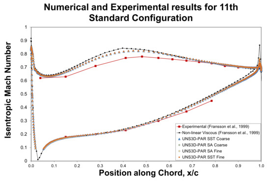
Figure 23. Measured and predicted Mach number on the eleventh standard configuration.

5. Conclusions

Four test cases were used to validate the implementation of the Shear Stress Transport and Spalart–Allmaras turbulence models in the UNS3D code. Two versions of the UNS3D code were considered: a sequential code, UNS3D-SEQ, and its parallel version, UNS3D-PAR. The validation of the implementation was done using experimental data and results generated by two NASA codes: FUN3D and CFL3D. The four cases considered were (i) a flat plate case, (ii) an airfoil near-wake, (iii) a backward facing step, and (iv) a turbine cascade known as the eleventh standard configuration. In all cases, the residuals of the solutions were less than 10${}^{-11}$. The numerical results generated by the UNS3D codes with the two turbulence models compared well with the experimental data and the results of NASA codes FUN3D and CFL3D. The two turbulence models produced similar results. Compared to the experimental data, the Spalart-Allmaras turbulence model did not predict the turbulent fluctuations and skin friction coefficient as well as the Shear Stress Transport turbulence model. The Spalart–Allmaras model predicted the velocity profiles better than the Shear Stress transport model as the flow moved away from the backward-facing step. Overall, the results generated with the Shear Stress Transport model were closer to the experimental data, the only exception being the prediction of the reattachment point on the backward-facing step, where the Spalart–Allmaras model outperformed the Shear Stress Transport model. The computational time of the Shear Stress Transport model solution exceeded that of the Spalart–Allmaras model by 4% to 38%. In addition, the solution generated by the Shear Stress Transport model was more sensitive to the far-field boundary conditions than that of the Spalart–Allmaras model.

References

- Jones, W.P.; Launder, B.E. The prediction of laminarization with a two-equation model of turbulence. Int. J. Heat Mass Transf. 1972, 15, 301–314. [Google Scholar] [CrossRef]
- Johnson, D.A.; King, L.S. A Mathematically Simple Turbulence Closure Model for Attached and Separated Turbulent Boundary Layers. AIAA J. 1985, 23, 1684–1692. [Google Scholar] [CrossRef]
- Wilcox, D.C. Reassessment of the Scale-Determining Equation for Advanced Turbulence Models. AIAA J. 1988, 26, 1299–1310. [Google Scholar] [CrossRef]
- Menter, F.R. Two-Equation Eddy-Viscosity Turbulence Models for Engineering Applications. AIAA J. 1994, 32, 1598–1605. [Google Scholar] [CrossRef]
- Spalart, P.R.; Allmaras, S.R. A One-Equatlon Turbulence Model for Aerodynamic Flows. In Proceedings of the 30th Aerospace Sciences Meeting & Exhibit, Reno, NV, USA, 6–9 January 1992. Number AIAA Paper 89-0366. [Google Scholar]
- Wilcox, D.C. Turbulence Modeling for CFD, 2nd ed.; DCW Industries: La Cañada, CA, USA, 2000. [Google Scholar]
- Allmaras, S.; Johnson, F.; Spalart, P. Modifications and clarifications for the implementation of the Spalart-Allmaras turbulence model. In Proceedings of the Seventh International Conference on Computational Fluid Dynamics (ICCFD7), Big Island, HI, USA, 9–13 July 2012; pp. 1–11. [Google Scholar]
- Polewski, M.D. Time-Linearization of the Spalart-Allmaras Turbulence Model. Master’s Thesis, Texas A&M University, College Station, TX, USA, 2020. [Google Scholar]
- Kim, K.S. Three-Dimensional Hybrid Grid Generator and Unstructured Flow Solver for Compressors and Turbines. Ph.D. Thesis, Texas A&M University, College Station, TX, USA, 2003. [Google Scholar]
- Roe, P.L. Approximate Riemann Solvers, Parameter Vectors, and Difference Schemes. J. Comput. Phys. 1981, 43, 357–372. [Google Scholar] [CrossRef]
- Harten, A. Self Adjusting Grid Methods for One Dimensional Hyperbolic Conservation Laws. J. Comput. Phys. 1983, 50, 235–269. [Google Scholar] [CrossRef]
- Barth, T.J.; Jesperson, D.C. The Design and Application of Upwind Schemes on Unstructured Meshes. In Proceedings of the 27th Aerospace Sciences Meeting, Reno, NV, USA, 9–12 January 1989. AIAA Paper 89-0366. [Google Scholar]
- Venkatakrishnan, V. Convergence to Steady-State Solutions of the Euler Equations on Unstructured Grids with Limiters. J. Comput. Phys. 1995, 118, 120–130. [Google Scholar] [CrossRef]
- Carpenter, F.L. Practical Aspects of Computational Fluid Dynamics for Turbomachinery. Ph.D. Thesis, Texas A&M University, College Station, TX, USA, 2016. [Google Scholar]
- Dervieux, A. Steady Euler Simulations Using Unstructured Meshes. In Computational Fluid Dynamics; VKI Lecture Series 1985-04; Essers, J.A., Ed.; The von Karman Institute for Fluid Dynamics: Rhode Saint Genese, Belgium, 1985; Volume 1. [Google Scholar]
- Gargoloff, J.I. A Numerical Method for Fully Nonlinear Aeroelastic Analysis. Ph.D. Thesis, Texas A&M University, College Station, TX, USA, 2007. [Google Scholar]
- Anderson, J.D. Computational Fluid Dynamics: The Basics with Applications; McGraw-Hill: New York, NY, USA, 1995. [Google Scholar]
- Carpenter, F.L.; Cizmas, P.G.A. UNS3D Simulations for the Third Sonic Boom Prediction Workshop Part II: C608 Low-Boom Flight Demonstrator. In Proceedings of the AIAA Aviation Forum, Reston, VA, USA, 15–19 June 2020. [Google Scholar] [CrossRef]
- Blazek, J. Computational Fluid Dynamics: Principles and Applications, 1st ed.; Elsevier: Amsterdam, The Netherlands, 2001. [Google Scholar]
- NASA. NASA Turbulence Modeling Resource. 2019. Available online: https://turbmodels.larc.nasa.gov (accessed on 13 March 2019).
- Coles, D. The law of the wake in the turbulent boundary layer. J. Fluid Mech. 1956, 1, 191–226. [Google Scholar] [CrossRef]
- Nakayama, A. Characteristics of the Flow around Conventional and Supercritical Airfoils. J. Fluid Mech. 1985, 160, 155–179. [Google Scholar] [CrossRef]
- Driver, D.M.; Seegmiller, H.L. Features of a reattaching turbulent shear layer in divergent channel flow. AIAA J. 1985, 23, 163–171. [Google Scholar] [CrossRef]
- Fransson, T.H.; Jöcker, M.M.; Bölcs, A.A.; Ott, P.P. Viscous and Inviscid Linear/Nonlinear Calculations Versus Quasi-Three-Dimensional Experimental Cascade Data for a New Aeroelastic Turbine Standard Configuration. J. Turbomach. 1999, 121, 717–725. [Google Scholar] [CrossRef]
Publisher’s Note: MDPI stays neutral with regard to jurisdictional claims in published maps and institutional affiliations. |
© 2021 by the authors. Licensee MDPI, Basel, Switzerland. This article is an open access article distributed under the terms and conditions of the Creative Commons Attribution (CC BY) license (https://creativecommons.org/licenses/by/4.0/).