Abstract
Composite indicators (CIs), i.e., combinations of many indicators in a unique synthetizing measure, are useful for disentangling multisector phenomena. Prominent questions concern indicators’ weighting, which implies time-consuming activities and should be properly justified. Landscape fragmentation (LF), the subdivision of habitats in smaller and more isolated patches, has been studied through the composite index of landscape fragmentation (CILF). It was originally proposed by us as an unweighted combination of three LF indicators for the study of the phenomenon in Sardinia, Italy. In this paper, we aim at presenting a weighted release of the CILF and at developing the Hamletian question of whether weighting is worthwhile or not. We focus on the sensitivity of the composite to different algorithms combining three weighting patterns (equalization, extraction by principal component analysis, and expert judgment) and three indicators aggregation rules (weighted average mean, weighted geometric mean, and weighted generalized geometric mean). The exercise provides the reader with meaningful results. Higher sensitivity values signal that the effort of weighting leads to more informative composites. Otherwise, high robustness does not mean that weighting was not worthwhile. Weighting per se can be beneficial for more acceptable and viable decisional processes.
1. Introduction
The study of complex phenomena requires the adoption of frameworks enabling multisector assessment of a variety of aspects. A typical solution is provided by the use of composite indicators (CIs), i.e., combinations of many indicators often structured in nested hierarchical ensembles, in diverse fields of knowledge, including environmental science and sustainability [1], vulnerability and climate changes [2], socioeconomics [3], and engineering [4]. The design of CIs is a critical process, which presents scientific and technical issues, even though it cannot be reduced to a unique pass par tout procedure [5]. In the public domain, the criticalities are even more evident since CIs influence or enter decision-making support systems concerning the use of funding for addressing specific policies [6]. In this respect, CIs support the ranking of a set of entities (countries, counties, municipalities, homogeneous zones, etc.), termed decision-making units (DMUs), that can be positively or negatively affected by the consequential distribution of resources. Final rankings depend on the variety of choices adopted to frame the indicators, though. The selection of indicators is crucial—different pools of indicators lead to different CIs. In addition, the same indicators may be combined, according to different algorithms leading to different expression of the CI. Algorithms usually include two elements—(i) the rule of indicator aggregation and (ii) the weighting of the indicators (see the review by Greco et al. [7]). A CI can be adopted in decision making when it is reliable, i.e., it is stable. In the other way around, a lower robustness is a sign that the modified CI conveys new information and prompts further assessment of the reasons why some inputs influence the CI. Thus, the sensitivity of the CI versus the algorithms used for its design and construction should be accurately assessed [8]. Sensitivity analysis is a powerful instrument and can be used to address properly the Hamletian question concerning the opportunity to introduce the weights or not.
In the domain of landscape analysis and planning, several metrics have been designed and applied to the assessment of landscape fragmentation (LF), the phenomenon of subdivision of habitats in smaller and more isolated patches (see the review by Wang et al. [9]). LF jeopardizes the normal evolution of animal species since it reduces the home range, i.e., the possibility to move freely in a favorite habitat. LF can be triggered by natural and human drivers, such as the construction of infrastructures and settlements. The indicators of LF provide a useful indication to effectively addressing green-based urban and regional management and planning. In a scientific panorama, in which contributions on composite indicators of LF are still rare, De Montis et al. [10] propose the composite index of landscape fragmentation (CILF). CILF combines three LF indicators bearing the same importance (i.e., weight)—the infrastructural fragmentation index (IFI), the urban fragmentation index (UFI), and the mesh size density (Seff). This composite is applied to the assessment of LF processes through 51 landscape units of the island of Sardinia, Italy, and provides a basis for addressing defragmentation policies.
In this paper, we aim at presenting a weighted release of the CILF applied to the assessment of LF in Sardinia in 2003. We focus on the sensitivity of the composite to different algorithms combining three weighting patterns (equal weights, principal component analysis-based weights, and expert judgment-based weights) and three indicators aggregation rules (weighted average mean, weighted geometric mean, and weighted generalized geometric mean). We assess the sensitivity of the weighted CILF by measuring the volatility of the position in ranking assumed by the DMUs (i.e., the landscape units). Since the weighting implies a significant amount of extra work, we are interested in ascertaining whether the weighting—i.e., the time-consuming elaborations on the importance of the indicators—is a worthwhile exercise.
2. State-of-the-Art Summary
Many scientists have built and applied composite indicators to the assessment of complex phenomena in several domains. In addition, they often propose frameworks, in which indicators are aggregated and weighted, according to a variety of patterns. Additionally, they are confronted with the sensitivity of the composite upon the different ways they are obtained. With respect to application field, indicator algorithm structuring, and sensitivity analysis, we comment on the contribution provided by a selection of essays, which are scrutinized in Table A1 (in Appendix A), according to focus, composite and component indicators, method, data, and details about the weights.
A very prominent stream of research studies deals with sustainability. Babcicky et al. [1] illustrate the re-engineering of the environmental sustainability index (ESI). The equivalized ESI is obtained through a weighted summation and supplies a rank with higher robustness. Dulvy et al. [11] develop a marine biodiversity threat indicator, which was calculated from the weighted average of the threat scores of individual fishes species in each year. Foster et al. [12] construct a measure able to gauge the robustness of country rankings associated with some well-known composite indicators—the human development index (HDI), the index of economic freedom (IEF), and the environmental performance index (EPI). Zhou et al. [13] recalculate the HDI using a multiplicative optimization approach to reduce subjectivity in defining the weights for the sub-indicators. Hassan [14] focuses on the sustainability of a region by building the total index of sustainability (TIS). The composite is constructed through multi-attribute utility theory as a weighted summation, where the weights represent the marginal variation of preference corresponding to the change of an attribute value. Huang et al. [15] review nine urban sustainability indicators (USIs), with respect to the three pillars of sustainability—weak and strong sustainability, aggregation and weighting, and spatialization. Kurtener et al. [16] assess agricultural land suitability through a composite indicator obtained by applying fuzzy logic. Munda and Saisana [8] develop a sensitivity analysis of a composite indicator of regional sustainability with respect to different indicator aggregation patterns. The authors consider weighted linear formula, nonlinear and non-compensatory multicriteria analysis, and data envelopment analysis (DEA), which is used to extract the weights. Pert et al. [17] study vegetal conditions in Australia by building a 25-point scale composite threat index combining five indicators normalized with a five-point scale. The aggregation rule is the unweighted summation because the indicators are considered of equal importance.
Given the relevance of the topic for this paper, some studies focus on landscape. Paracchini et al. [18] assess rural landscape through the societal landscape awareness indicator. The composite is based on three dimensions and six indicators. The indicators are normalized according to the min–max formula and aggregated according to the unweighted summation. Schüpbach et al. [19] focus on the impact of individual farms on visual landscape quality in Switzerland, according to the agricultural life cycle assessment (ALCA). They build the composite landscape indicator (CLI) by combining two sub-indicators. The aggregation rule consists of the unweighted summation: sub-indicators are assigned the same importance.
Another important set of articles tackle the questions connected to climate change. Ahsan et al. [2] construct the socioeconomic vulnerability index (SeVI) to assess climate change vulnerability in southwestern coastal Bangladesh. SeVI is obtained by aggregating the component indicators into a unique measure through weighted summation. Bastin et al. [20] develop the directional leakiness index (DLI), a composite index based on remotely sensed imagery. A component indicator concerning the patch size is obtained through weighted summation considering the importance of each patch size class. Christensen et al. [21] focus on methods useful for weighting regional climate models (RCMs). The authors considered six model performance indices and examined three ways for combining them into one weight per regional climate model. Garriga and Pérez Foguet [22] propose a revision of the water poverty index (WPI). The new index is studied with a combination of different aggregation rules and weighting, and a sensitivity analysis is applied. Weights are obtained through expert judgment and multivariate (principal component) analysis. The best aggregation function implies a principal component analysis (PCA)-based selection of indicators and a weighted geometric mean of subindices. Machado and Ratick [23] consider the sensitivity of a composite index of vulnerability to flooding with respect to four aggregation rules—weighted linear combination (WLC), ordered weighted average (OWA), DEA, and compromise programming (CP). Salvati and Zitti [24] focus on land degradation by applying the land vulnerability index (LVI). LVI combines three dimensions and nine indicators, according to the weighted summation rule. Szlafsztein and Sterr [25] build the coastal vulnerability index (CVI) to assess the vulnerability of coastal zones. CVI combines two dimensions through an unweighted summation. Each dimension is obtained as weighted summation aggregation of 16 indicators.
The next cluster gathers essays concerning socioeconomic issues. Busu and Busu [3] construct the Shannon entropy composite index (SECI). The SECI is obtained as a weighted summation of simple indicators processed through an algorithm based on Shannon entropy. Lee and Lim [26] propose a composite for forecasting the daily change of the Korea composite stock price index (KOSPI). Manthalu et al. [27] focus on a composite indicator obtained through a weighted summation of 27 indicators. Weights are calculated through PCA. Rahman [28] analyses the sensitivity of a quality of life index (QOLI) to two aggregation and weighting patterns—the first, a PCA-based weighted summation, and the second, the unweighted summation of Borda scores. The composite combines eight indicators and is calculated for 43 developing countries. Ferrant et al. [29] evaluate gender inequality through the multidimensional gender inequality index (MGII). The MGII is obtained as a weighted summation of the squares of subcomponent indices measuring eight dimensions of inequality.
The last group of essays attains engineering. Gerpott and Ahmadi [4] propose a revision of the Information and telecommunication technologies development index (IDI), a composite showing 3 sub-indices and 11 indicators. This study aims at tuning the set of weights to maximize the reliability of IDI, with respect to its ability to gauge the achievement of socioeconomic targets. Gitelman et al. [30] study a composite index that combines the main dimensions characterizing the road safety pyramid. The authors combine the indicators applying principal component analysis and factor analysis to obtain weights in five trials. Rocco et al. [31] develop a composite indicator by considering the ordered weighted averaging aggregation approach. Sharifuddin [32] focuses on the energy security index (ESI) combining five dimensions (availability, stability, affordability, consumption efficiency, and environmental impact), 13 elements, and 35 indicators. Indicators, elements, and dimension scores are normalized between 0 and 1 and aggregated according to unweighted summation for every level but the indicator tier. Shen et al. [33] construct a composite road safety performance indicator, combining seven indicators through normalization in the interval 0–1 and weighted summation aggregation rule.
The analysis of the literature provides the reader with some leitmotiv that is worth being recalled. Oftentimes, scientists have attempted to revise and re-engineer already existing composite indicators with more sophisticated algorithms, including the introduction of weights meant as the importance of the indicators. This has implied usually a great methodological and applicative effort, which has not necessarily led to a better or finer release of the composite. A variety of weighting frameworks has been adopted to extract figures representing the importance of each indicator: some methods focus on the percentage share of information embedded in each indicator, while others on the elaboration of the judgment of selected experts. The weighting is a relevant part of the indicator aggregation rule that can be compensatory, i.e., allowing the balancing of opposite performances in two or more indicators, or not. A cornerstone phase of the composite indicator assessment consists of the sensitivity analysis, which scrutinizes the changes of the output, i.e., the final ranking, with respect to the variation of the input, i.e., the weighting and aggregation patterns. If the changes are negligible, the ranking is stable, and the composite is robust. As a corollary, if the comparison of the resulting ranking of a composite with its weighted release reveals low volatility, the weighted composite does not add much to the picture already provided by the unweighted composite indicators. Otherwise, in presence of high sensitivity, the analyst deals with a weighted composite that describes a richer outline of the phenomenon at hand. This is clearly a sign that the weighting effort has been worthwhile.
3. Methods
The experimented method is a complement of the framework presented by De Montis et al. [10], who build, apply, and evaluate the robustness of the composite index of landscape fragmentation (CILF) with respect to the volatility of the ranking of 51 landscape units (LUs) established by the Regional Landscape Plan of Sardinia (RLP) [34]. De Montis et al. [10] (i) considered a complete spatial data set, which consisted of human settlements and transport and mobility infrastructures (roads and railways), (ii) applied the generalized geometric mean (GGM) as aggregation algorithm, and (iii) performed a sensitivity analysis of the findings to assess the robustness of CILF.
CILF is designed as a three-indicator unweighted composite, according to the scheme proposed by the Organisation for Economic Co-operation and Development (OECD) [35] and Nardo and Saisana [5]. The scheme includes the following steps: theoretical framework, variables, normalization, aggregation, and robustness and sensitivity [10]. Since we now focus on a weighted release of the CILF, we add a new step concerning the assessment of values representing the importance of the indicators. The simulated theoretical framework consists of aiding a decisional process, in which stakeholders are interested in managing landscape fragmentation starting from a unique simple measure (namely, the CILF) melting three major determinants, i.e., transport and mobility infrastructures, human settlements, and subdivision per se. The indicators selected for measuring those determinants are the infrastructural fragmentation index (IFI), the urban fragmentation index (UFI), and the effective mesh density (Seff). In Table 1, we resume their main characteristics and rationales.

Table 1.
Synopsis of the indicators combined in the composite index of landscape fragmentation (CILF) (after De Montis et al. [10]).
Variables have been calculated by applying advanced geographical analysis and processing spatial data sets in shapefile in the GIS environment provided by QGIS (https://www.qgis.org/it/site/) and standard spreadsheet programs (Microsoft Excel). Information concerning the geography of Sardinia and—typically—polygonal elements was obtained by processing the land use map available for free at the institutional website of the regional administration. Sardinia Geoportal is the interface of the regional geographic information system and the related spatial data infrastructure.
Indicators are expressed in different measurement units and need to be normalized. In this case, we chose the min–max transformation rescaling the original values into figures calculating the distance from the minimum normalized with respect to the range of the original indicator. We selected this model because it was chosen by De Montis et al. [10] for designing the baseline release of the CILF.
The next step concerns the indicator weighting, where components are attributed a value measuring the relevance of the issue represented by the indicator. As often presented in the literature, weights are obtained according to two main procedures—quantitative statistical calculations and expert judgment. The first procedure implies the scrutiny of the matrix of indicator values through multivariate statistical analysis, for instance, the widely adopted in the literature principal component analysis (PCA) and factor analysis (FA), and the association of weights values to each indicator depending on the percentage share of variance explained. In this respect, weights are referred to the variable loading calculated by means of factor analysis for the prevalent (i.e., explaining most of the variance) component. This procedure is based on the analysis of the results of an online questionnaire proposed to a panel of selected individuals. The survey aims at understanding the characteristics of the sample (position, age, education, familiarity with LF) and the importance attributed to each indicator. Interviewees are requested to express the level of importance, according to a five-step Likert-type scale (very low, low, medium, high, and very high). This method was introduced in psychology by Likert and is currently widely used [43,44,45]. Following El Gibari et al. [46], the weights for the ith indicator are extracted by (i) calculating the arithmetic mean of the judgments mwi; (ii) computing the adjusted weights defined as awi = 1.5(mwi−1) to be applied in a multiplicative environment, where the ratio between two consecutive elements of the Likert-type scale is constant and equal to 1.5; and (iii) rescaling the adjusted weights so that they sum up to 1.
The next step consists of the selection of the patterns of indicators’ aggregation. We used the weighted version of three algorithms selected by De Montis et al. [10] for the CILF, as detailed in Table 2.
Table 2.
The indicators' aggregation rules used for designing the weighted release of the CILF*.
The three algorithms are designed to yield composite indicators with full (weighted arithmetic mean (WAM), no (weighted arithmetic mean (WGM), and partial (weighted generalized geometric mean (WGGM) compensation between the indicators. WGGM-based aggregation rules merge compensatory (i.e., an increase of one indicator can be balanced by the decrease of another indicator) and non-compensatory frameworks [47]. The parameter β is set greater than zero and attaining a maximum of 1 (corresponding to the arithmetic mean allowing full compensation among the indicators). Following De Montis et al. [10], we chose an intermediate framework by setting β = 0.50.
The final step regards sensitivity analysis to ascertain the level of robustness of the composite with respect to different weighting and aggregation patterns. We performed sensitivity analysis by verifying the variability of the position occupied by each decision-making unit (DMU), according to the various rankings resulting from the different composites obtained. Since we are interested in the variation of the position in the ranking and not in its increase or decrease, we slightly modify what was proposed in other studies [10,48]. Thus, we set as a general measure of divergence GD between two rankings the absolute value of the average shift in the ranking (GD = |ASR|), where |ASR| obeys the following formula:
where m is the number of DMUs, and Ranki1 and Ranki2 stand for the position occupied by the i-th DMU, according to composite 1 and, respectively, composite 2. The higher the GD is, the higher the sensitivity of the CI to changes in the way indicators are weighted and aggregated; otherwise, the lower the GD, the higher the robustness. Final outcomes do not change much when selecting different frameworks. However, statistics that suggest, on average, a given outcome are many times partially or totally contradicted by the analysis of average shifts in the ranking (|SR|) reported by individual DMUs. Thus, we add the study of measures of specific divergence (SD), namely, the maximum absolute shift in the ranking (|SR|max), the share of higher than five positions absolute shifts in the ranking (|SSR|>5), and the share of higher than 10 positions absolute shifts in the ranking (|SSR|>10). These metrics provide the analysts with detection of the DMUs mostly affected by selecting a given CILF expression versus another one. The higher the SD matrices are, the higher the volatility of the CILF selected with respect to other composites.
4. Application and Results: A Weighted Composite Indicator of Landscape Fragmentation
In this section, we apply the methodology explained above to the assessment of a weighted release of the CILF. We simulate a decisional environment, where relevant stakeholders—including the Autonomous Regional Administration—are interested in managing LF in the 51 (27 coastal and 24 internal) LUs established by the RLP [34], the main strategic regional plan of Sardinia, Italy (Figure 1A). Sardinia shows a surface area of about 24,000 km2; thus, is the second largest Italian island. The island is scarcely populated, however, since it has about 1.6 million inhabitants. Sardinia is an autonomous region with special power in landscape management and planning. Decision makers can be assisted by the interpretation of the values CILF of the LUs, which are selected as decision-making units (DMUs) of this exercise; the spatial pattern of the LUs is illustrated in Figure 1B. While De Montis et al. [10] monitored the variation from 2003 to 2008, we refer just to the initial year 2003 for comparing the unweighted CILF to two weighted releases. Indicators have been obtained by processing spatial information described in Table 3.
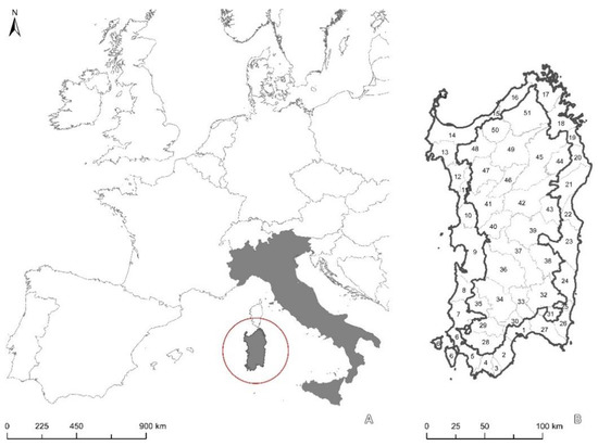
Figure 1.
(A) The red circle identifies the location of Sardinia (Italy), in the context of the western Mediterranean basin. (B) The decision-making units consist of the 51 landscape units of the RLP of Sardinia. The thick line divides coastal from interior LUs.
Table 3.
Spatial data set used for calculating the indicators of landscape fragmentation (LF).
Indicator values have been normalized, according to the min–max transformation, and projected in the range of 0–1.
Weights have been obtained, according to the two methods, and are reported in Table 4.
Table 4.
Indicators weights obtained by extraction method.
The second set of weights has been computed by applying PCA to the min–max normalized values of the indicators. A preliminary check of the determinant (equal to 0.48) indicates that the structure of the dataset justifies the application of PCA. The Keiser–Meyer–Olkin (KMO) test (suitability measure equal to 0.34) reveals a limited utility of PCA; this is expected for a dataset with a reduced number of variables. The Bartlett test (significance equal to 0) indicates that the variables are poorly correlated. We have extracted three components, as reported in Table 5.
Table 5.
Components extracted by initial eigenvalue and percentage of variance explained.
Component 1 explains the largest share of variance (nearly 54%) and has been selected for the extraction of the variable loading values for the indicators, as indicated in Table 6.
Table 6.
Variable loading values obtained for component 1.
Variable loading values have been normalized in the triplet reported in Table 4 so that their sum is equal to 1.
The third set of weights has been obtained by processing the results of an online questionnaire submitted to selected stakeholders in January 2021. The link to the questionnaire was sent to scientists of the two universities of Sardinia, public officials belonging to Sardinian municipalities, and associates to the professional boards of the engineers of the province of Cagliari and agronomists of the provinces of Sassari and Oristano. The questionnaire was completed by 165 individuals. Most of them were academics (45%), freelance professionals (31%), and public officials (15%). The sample includes persons 36–50 (40%) and 51–65 (44%) years of age. The level of education was generally high: 53% of the respondents held a masters’ degree and 45% a post lauream degree. Most of the respondents (50%) declared to have a medium level of acquaintance with LF, 25% a high level, 16% a low level, while 8% admitted having never heard of the concept. Weights vary depending on the many segmentation of the audience interviewed because academics may have a different perception of the phenomenon, compared to freelance professionals. In this study, we do not inspect these variations.
In Table A2 in Appendix B, we gather the values of the CILF obtained for 2003, with min–max normalization of the indicators, and different combinations of weighting and aggregation rules. We now apply sensitivity analysis to understand the volatility of the various rankings focusing on two issues, namely, (i) the influence of weighting patterns, being equal the aggregation rule and (ii) the influence of aggregation rules, being equal the weighting pattern. The resulting figures are shown in Table A3 in Appendix B, where the detailed absolute values of the shift in rankings are reported for each DMU. In Table 7 and Table 8 and Figure 2 and Figure 3, we report the GD and SD metrics.
Table 7.
Sensitivity analysis of CILF (2003). Rankings are compared pairwise keeping fixed the aggregation rules and changing the weighting patterns.
Table 8.
Sensitivity analysis of CILF (2003). Rankings are compared pairwise keeping fixed the weighting patterns and changing the aggregation rules.
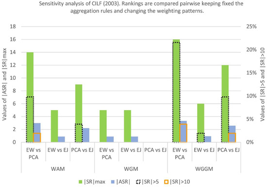
Figure 2.
Sensitivity analysis chart of CILF (2003). Rankings are compared pairwise keeping fixed the aggregation rules and changing the weighting patterns.
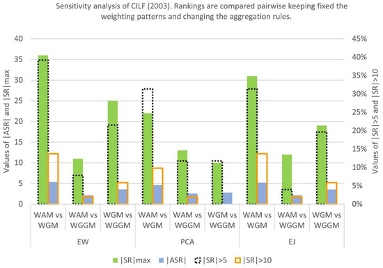
Figure 3.
Sensitivity analysis chart of CILF (2003). Rankings are compared pairwise keeping fixed the weighting patterns and changing the aggregation rules.
The analysis of the |SR| indicates that the less volatile aggregation rule is the WGM—in this domain, the most robust comparison concerns the interplay between composites obtained with weights extracted through PCA and expert judgment elaboration. In this case, |ASR|, |SR|max, |SR|>5, and |SR|>10 are equal to 0. Slightly higher figures are associated with the other two comparisons within the WGM aggregation rule and the equal weight (EW) vs. expert judgment (EJ) comparisons within the WAM and the WGGM aggregation rules. The most volatile interplays are EW vs. PCA comparisons with WGGM and WAM aggregation rules.
As for the assessment of the impact of the change of aggregation rule keeping the weighting patterns fixed, much higher figures are obtained—a clear sign of a higher sensitivity of the resulting rankings to the different ways the indicators are weighted. The most robust is the WAM vs. WGGM comparison with EW and EJ weighting patterns, even though |SR|>5 = 7.84% is a sign of local perturbations. The most volatile comparison is WAM vs. WGM with the EJ weighting pattern.
5. Discussion
In this section, we discuss the outcomes of this paper with respect to the premises presented in the introduction.
First, in the framework of the assessment of LF throughout Sardinian LUs, we are interested to check whether the weighted versions of the CILF perform better—i.e., add more information—than its unweighted releases (all weights equal). We would like to stress that the development of both weight assessments implies demanding and time-consuming activities, such as the mobilization of scientific knowledge, the application of sophisticated methods and algorithms, the design, test, and submission of ad hoc questionnaires, the selection of the target audience, etc. Weighting is never for free because it implies costs, which are also difficult to evaluate precisely in advance. Thus, it is not surprising that scientists question the worthiness of the weighting effort. In our exercise, we obtained the weights following two streams of research. According to the first set of contributions (for instance, Huang et al. [15]), we opted for an “objective” quantitative assessment of the importance of the indicators, which are calculated as the percentage of variance (information) explained. This is an informational weighting method that yields values by processing characteristics embedded in the indicators’ dataset. The PCA-based triplet of weights reported in Table 4 signs a clear prevalence of IFI and UFI with respect to the Seff. This per se diverges from the scenario represented by the equalization of the weights. According to a stream of contributions (see [43,46]), we have calculated another weight triplet applying a “subjective” assessment that considers the judgment of a set of selected experts. This triplet is representative of the average judgment of the experts and may vary when considering a different set of participants. The endorsers of subjective assessment frameworks question that quantitative PCA-based methods may be too neutral and abstract for policy and decision makers. In addition, they point out that a clear presentation of subjective assessment methods may strengthen the acceptability and viability of weighted CIs. In our case, the expert judgment-based weight triplet (see Table 4) converges to the scenario with all weights equal. Therefore, an argument purely focused on the values of the weight triplets would suggest that the first process of weighting was more worthwhile than the second because the first one potentially leads to a different picture with respect to the situation described by the unweighted CILF (all weights equal). However, we need to widen our perspective to complete the assessment of the influence of the algorithm on the new release of the CILF. Thus, we have jointly analyzed the combined impacts of both the weighting pattern and the aggregation rule.
Therefore, as for the argument concerning the evidence of the complete sensitivity analysis, it does not show us a monochrome picture and needs to be carefully interpreted. If we consider the outcomes reported in Table 7 and Table 8, the figures do not address a monolithic message. In the first case, figures suggest that sensitivity is overall contained (|ASR| < 2.98 and many other SR statistics equal to zero). The high robustness emerging is a sign that—keeping the aggregation rule constant—CILF is not sensibly affected by changes in the weighting pattern. Thus, from this point of view, the weighting effort was not worthwhile. Similar evidence has been discussed by some of the selected contributions (by, for instance [12,21]). A different picture arises when we consider the outcomes reported in Table 8. In this case, sensitivity measures show a much higher range (|ASR| < 5.39, |SR|max < 36, |SR|>5 < 39.22%, and |SR|>10 < 13.73%). This means that keeping the weighting patterns constant and allowing changes in aggregation rules produce sensibly different rankings. Therefore, under these lenses, weighting was a worthwhile process, as documented by another set of selected contributions ([1,4,22]). In line with what Foster et al. [12] found for the weighted releases of the HDI, IEF, and the EPI, the exercise developed in this paper documents a controversial outcome: some CIs are robust and some others are not. This means that weighting is sometimes (i.e., for some releases of the weighted CILF) justified, while at other times, is not.
6. Conclusions
In this paper, we have developed the Hamletian question revolving on whether to introduce weights or not in the design of composite indicators. We examined the impact of using two weighting extraction modes on the CILF, an unweighted composite indicator proposed by De Montis et al. [10] for measuring landscape fragmentation. We have focused on the sensitivity of the CILF to different indicator aggregation rules and weighting patterns. The analysis provides us with twofold outcomes. Even though high sensitivity is associated with lower robustness, in our case, it signals that the new composite conveys richer information, i.e., that the weighting has been worthwhile. The analysis of the SR statistics reveals higher values when rankings are compared pairwise changing aggregation rules and fixing the weighting patterns (Table 8). In this case, the weighted versions of the CILF embed new information and lead to different rankings—a circumstance that justifies the adoption of the composites and the effort for introducing the weights. The cases reported in Table 7 describe a panorama, in which low sensitivity values would support that the new weighted composites do not add much to the information provided by the original CILF and that the weighting has not been worthwhile.
However, this can be questionable since weighting per se adds advantages, as intangible as they may be. There are processual benefits connected to a procedure based on composites with weights extracted through both PCA and EJ. PCA provides important indications on the structure of the information contained in the indicators and may support the choice of “objective” weights. EJ-driven weights convey per se a powerful symbolic meaning, which can increase political awareness and endorsement for the widest possible viability of the composite. This holds also in our case, where the weights triplet obtained with EJ does not diverge much from the EW triplet. Still, it represents the combination of the opinions of many individuals representing sometimes the sentiment of relevant political parties or stakeholders. EJ-driven weighted composites often are accepted with higher appreciation in deliberative contexts, where PCA-based weights may be perceived as abstract constructs of meaningless technicality.
As a general message, this paper confirms that the design of a composite indicator is context specific and never a neutral activity and weighting processes are time and resources consuming. The main practical implication is that the cornerstones of the procedure must be clarified step by step so that the audience (institutional partners, decision-makers, stakeholders, etc.) can adhere to and use the composite indicator with full awareness of its impacts. In this respect, the development and correct communication of sensitivity analyses are fundamental.
In this study, we have developed the analyses under precise assumptions; thus, the outcomes have some limitations we would like to clarify for departing with further research studies. Firstly, we have tested the method on the CILF, a composite combining three indicators. The method—with the same steps and procedures—can be exported to other composites, but the results may be affected by the different structure of the indicator nesting and pattern and some adjustments may be required. Additionally, PCA statistics vary, in front of a higher number of indicators; and the extraction of EJ-driven weights may lead to diverse patterns when judging the importance of a larger number of indicators. Secondly, we have considered the CILF proposed by De Montis et al. [10] as a possible combination of three out of all the available measures of LF. However, we are aware that different formulations of the CILF may be obtained by including a larger number of indicators with a multi-layer nested structure. Thirdly, we have addressed the weighted CILF by choosing the min–max rescaling of the original indicators. Different courses of action would have followed a selection of alternative normalization patterns (Borda distance, standardization, ratio to the maximum, etc.). Similarly, we have focused on the GGM aggregation rule calibrated on a fixed compensation parameter β. We are aware that sensitivity analysis can be directed also to the assessment of the interplay between the composite and a changing compensation of the indicators. We will delve into this in future studies. Fourthly, EJ weights are extracted through the method proposed by El Gibari [46] and the Likert scale. Other methods can be selected for processing expert judgment (see, among others, the regime method by Hinloopen and Nijkamp [49], the analytical hierarchy process by Saaty [50], and goal programming and DEA methods [51,52]). This choice has its impacts on the entire study, which would have implied different data harvesting procedures and outcomes with the selection of a different EJ processing framework. Fifthly, regardless of the EJ processing pattern, we have extracted a unique weight triplet from the consideration of the entire dataset of answers provided by the experts. However, experts can be profiled by profession, age, education, and familiarity with LF issues in different clusters, which may be associated to many corresponding weight triplets. Finer sensitivity analyses may be applied to understand the influence of experts profiling on the weights and, overall, on the composite indicator. In addition, the sample was designed for including academics and professionals, i.e., individuals with a presumably medium-high familiarity with technical aspects connected to LF management and planning. However, this composition could not correspond to the characterization of a typical deliberative body operating in the public domain, where the share of decision makers with no exposure to LF issues might be greater. Further research will be directed to seek the most suitable profile of candidate stakeholders.
Author Contributions
Conceptualization, A.D.M.; methodology, A.D.M.; formal analysis, V.S. and D.T.; investigation, A.D.M., V.S., G.C., D.T. and A.L.; data curation, V.S., D.T. and G.C.; writing—original draft preparation, A.D.M.; writing—review and editing, A.D.M. and A.L.; supervision, A.D.M. All authors have read and agreed to the published version of the manuscript.
Funding
The Authors are supported by the research project “Paesaggi rurali della Sardegna: pianificazione di infrastrutture verdi e blu e di reti territoriali complesse [Rural landscapes of Sardinia: planning green and blue infrastructures and spatial complex networks]”, Regional Law n. 7/2007, Fund for Development and Cohesion, Autonomous Region of Sardinia.
Institutional Review Board Statement
Not applicable.
Informed Consent Statement
Not applicable.
Data Availability Statement
Not applicable.
Acknowledgments
Andrea De Montis and Antonio Ledda are supported by the University of Sassari through the Fondo di Ateneo per la Ricerca [Academic funding for research activities] 2020. Giovanna Calia gratefully acknowledges the financial support of her scholarship for the PhD program in Civil Engineering and Architecture (University of Cagliari) by P.O.R., F.S.E. Operational Programme 2014–2020, Autonomous Region of Sardinia.
Conflicts of Interest
The authors declare no conflict of interest. The funders had no role in the design of the study; in the collection, analyses, or interpretation of data; in the writing of the manuscript, or in the decision to publish the results.
Appendix A
Table A1.
Scrutiny of relevant essays by focus, composite and component indicators, method, data, and details about the weights.
Table A1.
Scrutiny of relevant essays by focus, composite and component indicators, method, data, and details about the weights.
| Author (Year) | Focus On | Composite and Component Indicators | Method | Data | Details about the Weights |
|---|---|---|---|---|---|
| Ahsan and Warner [2] | Vulnerability to climate change. | Socioeconomic Vulnerability Index (SeVI) combining three dimensions (adaptive capacity, sensitivity, and exposure), 5 domains, and 27 indicators. | Qualitative approach to the Rapid Rural Appraisal and discussion in seven focus groups. SeVI is obtained as weighted average of the three dimensions and is normalized in the interval 0–1. | Data on communities in south-western coastal Bangladesh was collected through household survey on vulnerability aspects: demography, society, economy, perception of climate risk, and geography. | The weights of the dimensions are obtained through follow-up workshops. |
| Babcicky et al. [1] | Sustainability. | Equivalised Environmental Sustainability Index (ESI). ESI combines three out of the five components of the original ESI and 10 variables. | Equivalised ESI is a weighted release of the original composite indicator ESI. | Most recent 2005 ESI data for world countries. | Weights are calculated through factor analysis. |
| Bastin et al. [20] | Landscapes function to retain resources. | Directional Leakiness Index (DLI) including four dimensions gauged by landscape metrics: landscape leakiness index, weighted mean patch size, lacunarity index, and proximity index. | DLI is obtained as a linear weighted summation of the dimensions. | Images drawn from Specterra Systems digital multi-spectral video (DMSV), whose spatial distortion is removed through automated techniques. | In the weighted mean patch size, a weight for each patch size class is computed. |
| Busu and Busu [3] | Circular economy processes. | Shannon Entropy Composite Index (SECI) combining recycling rate and economic growth of the EU member states. | The SECI is obtained following four steps: data standardization, weights computation, weights standardization, and ranking. | The data on 28 European member states are drawn from The Statistical Office of the European Union. | Weights represent the importance of the component indicators. |
| Christensen et al. [21] | Weighting regional climate models (RCM). | Combining individual metrics (indices) into one weight per RCM. | Model weighting grounded on multiple performance metrics in an ensemble of RCM simulations. | Reference datasets processed in 15 simulations at 13 institutes for the metrics: ERA40, CRU TS1.2, and EOBS2.0. ISCCP-D2. | RCM weights are obtained through six model performance metrics. Total weight is processed in three different ways. |
| Dulvy et al. [11] | Marine biodiversity loss. | Composite indicator of threat including rate and extent of decline. | Indicators are aggregated through weighted summation. | Data on 23 see fish species are drawn from the North Sea English groundfish survey data for 1982–2001. | Individual species threat categorizations were weighted as vulnerable = 1, endangered = 2, and critically endangered = 3. |
| Ferrant et al. [29] | Gender inequality. | The Multidimensional Gender Inequalities Index (MGII) considers eight dimensions (identity, physical integrity, intra-family laws, political activity, education, health, access to economic resources, and economic activity) and many variables. | MGII is obtained as weighted summation of the squares of the dimensions. Dimensions are gauged by correlation analysis (Kendall Tau-B test), standardization, aggregation (via unweighted summation), rescaling in the interval 0–1. | Data on 109 developed and developing countries are drawn from Women’s Indicators and Statistics Database of the United Nations, Cingranelli-Richards (CIRI) Human Rights Data, World Bank Development Indicators, and Gender Development and Institutions (OECD). | Weights are extracted through Multiple Correspondence Analysis (MCA) and mean the relative share of variance explained by each dimension. |
| Foster et al. [12] | Robustness analysis of Composite Indices versus different sets of weights. | Robustness analysis is applied to three indices: the Human Development Index (HDI) with three subcomponents, the Index of Economic Freedom (IEF) with 10 subcomponents, and the Environmental Performance Index (EPI) with various level of aggregation. | Dominance and prevalence analyses are applied to assess the type of dominance relation between two countries. Full dominance (C0) is established if the order in ranking cannot be reversed by using any set of weights. Otherwise, dominance relation (Cr) holds, only if a subset of weights is selected. The measure of robustness (r*) ranges between 0 and 1 (for fully robust relations). To consider all the comparisons, a prevalence function p(r) is considered based on the entire cumulative distribution of robustness levels. P(r) is the proportion of comparisons, for which Cr applies: for C0, p(0) = 1. | HDI data for 177 countries in 1998 and 2004. IEF for 157 countries in 2007. EPI for 149 countries in 2007. | All possible combinations of weights are considered. |
| Garriga and Pérez Foguet [22] | Sensitivity analysis of composite indicators of water stress and scarcity. | Water Poverty Index (WPI) with five dimensions: resources, access, capacity, use, and environment. | Sensitivity analysis is applied to assess the variability of WPI vs. aggregation and weighting patterns. The best combination implies a PCA-based selection of indicators and a weighted geometric mean of subindices. | Data on Turkana district, Kenya are drawn from the Government of Kenya and UNICEF (2006). | Weights are obtained by expert judgment and principal component analysis. |
| Gerpott and Ahmadi [4] | Sensitivity analysis of a composite indicator of the Status of Information and Telecommunication Technologies (ICT). | ICT Development Index (IDI) by the International Telecommunication Union (ITU). IDI includes three sub-indices and eleven indicators. | A revision of the IDI is proposed by means of partial least squares (PLS) and structural equation modeling (SEM) techniques. A sensitivity analysis is applied to investigate the variability of the rank with respect to weighting and aggregation. | ITU World Telecommunication/ ICT Indicators database. Statistics and supplemented by estimates which were provided by the ITU in case that the UNESCO files did not contain an indicator value. | Weights are calculated to minimize the difference between the IDI and the growth rate of the gross domestic product per capita. |
| Gitelman et al. [30] | Road safety. | The composite index of country road safety combines four dimensions and many indicators: policy performance (road safety programs), final road safety outcomes (fatality rates, scope of traffic injury), intermediate outcomes (wearing rates of seat belts, crashworthiness, and composition of vehicle fleet, alcohol-impaired driving), and background characteristics of countries (motorization level, population density). | The composite combines the main layers of the road safety pyramid and is obtained by applying PCA and Factor Analysis in five trials. | Data on 27 European countries are drawn from various databases maintained by the European Transport Safety Council, and Organization for Economic Co-operation and development, International Transport Forum. | Weights are extracted through Principal Component Analysis and Common Factor Analysis. |
| Hassan [14] | Sustainability of a region. | Total Index of Sustainability (TIS) is based on three indicators (economy, society, and environment), which include several criteria. | Multi-attribute utility theory is applied to construct the TIS as a weighted summation. | Data on GDP, solid waste, income disparity, and crime rate. An example for three countries is made. | The weights represent the change in the strength of preferences as an attribute varies from the worst to the best level. |
| Huang et al. [15] | Urban sustainability. | Nine Urban Sustainability Indicators (USIs): Ecological Footprint (EF), Green City Index (GCI), City Development Index (CDI), Environmental Performance Index (EPI), Genuine Progress Indicator (GPI), Genuine Savings (GS), Human Development Index (HDI), Happy Planet Index (HPI), Wellbeing Index (WI), Sustainable Society Index (SSI). | USIs are reviewed and classified, with respect to the three pillars of sustainability, weak and strong sustainability, aggregation and weighting, and spatialization. | No specific data set is recalled nor used. | In some cases (CDI, EPI, SSI, and WI), the aggregation rule is the weighted average. Whenever possible, quantitative methods (PCA, FA, DEA, AHP, CA) are recommended to calculate weights. |
| Kurtener et al. [16] | Agricultural land suitability. | Combined Fuzzy Indicator (CFI) is obtained as an aggregation of Individual Fuzzy Indicators (IFIs) including concentration of carbon (C) and phosphorous (P). | The method follows a typical fuzzy logic framework with phases for structuring, fuzzy modeling, computation, and evaluation. | Data from an experimental agricultural field on the Elm Creek watershed in Bell County, Texas (USA). | CFI is obtained through weighted summation of IFI values. |
| Lee and Lim [26] | Forecasting the change of the daily Korea composite Stock Price Index (KOSPI). | The composite is obtained processing values of three basic indicators: Relative Strength Index (RSI), Commodity Channel Index (CCI), and Current Price Position (CPP). | The authors apply the non-overlap area distribution measurement method based on the neural network with weighted fuzzy membership functions (NEWFM). | KOSPI data drawn from 2928 trading days from January 1989 to December 1998. | The weights are calculated according to the NEWFM. |
| Machado and Ratick [23] | Prioritizing mitigation and adaptation strategies for reducing the vulnerability to global environmental change (GEC). | Composite index of vulnerability to flooding based on the combination of three dimensions (exposure, sensitivity, and adaptive capacity) and six constituent indicators, i.e., exposed population, exposed area, forecasted frequency of floods, landscape disturbance, protection from financial loss, and financial resources. | Review of four aggregation rules: Weighted Linear Combination (WLC), Ordered Weighted Average (OWA), Data Envelopment Analysis (DEA), and Compromise Programming (CP). | An example is set to assess vulnerability to flooding of 48 hydrological subregions in northeastern United States. Many datasets are considered to construct the constituent indicators including the National Land Cover Database, US Census, and National Flood Insurance Program dataset. | Weights are calculated according to the four aggregation rules. |
| Manthalu et al. [27] | Socio-economic status for addressing resource allocation by the health care system. | Composite indicator of need including 27 indicators clustered in 6 dimensions. | The composite is obtained by aggregating the indicators through a weighted summation rule. | Malawi Multiple Indicator Cluster Survey (2006). | Weights are calculated by PCA. |
| Munda and Saisana [8] | Sensitivity of indicators of regional sustainability. | Composite indicator of regional sustainability with a tree nested framework including three dimensions (environment, society, and economy) and 29 indicators. | Sensitivity analysis is applied to assess the variability of resulting rankings obtained through different aggregation rules: weighted linear summation, nonlinear and non-compensatory multicriteria analysis, and data envelopment analysis (DEA). | Data on Spanish, Italian and Greek 25 NUTS 3 areas are drawn from the regional database REGIO of Eurostat and the Spanish National Statistical Office. | Weights (importance of the indicators) are region-specific and are calculated through DEA. |
| Paracchini et al. [18] | Agricultural landscape. | Societal landscape awareness indicator with three dimensions (protected areas, rural tourism, and quality of products) and six indicators. | The dimensions are normalized to a 0–10 range with min-max transformation. Aggregation rule consists of the unweighted average. Two case studies are developed for Europe (NUTS2 level) and the region of Alentejo, Portugal (LAU12 level). | Indicators are nurtured by several datasets on Natura2000 sites, World Heritage UNESCO sites, European nationally designated areas, International Union for Conservation of Nature category V—World Protected Areas: CORINE 2000 land cover map, Farm Structure Survey (Eurostat), Farm Accountancy Data Network (European Commission), the DOOR database (European Commission), and the database on VQPRD wines (European Commission). | Dimensions and indicators have the same weight. |
| Pert et al. [17] | Vegetation conditions. | Composite threat index combining five indicators: fragmentation of forest cover, urbanization, weeds, feral animals, and road density. | The indicators are normalized in a five-point scale and aggregated through unweighted summation in a twenty-five-point scale composite indicator value. | Datasets include Landsat 7 satellite imagery, satellite images, density of weed species, feral animals, and roads. | Indicators have the same importance. |
| Rahman [28] | Sensitivity analysis of indicators of quality of life. | Quality of Life Index (QOLI) combining eight indicators (causal variables): per capita income, life expectancy at birth, infant mortality rate, prevalence of child malnutrition, access to sanitation, access to safe drinking water, adult illiteracy rate, and the per capita commercial energy use. | The sensitivity analysis of QOLI with respect to two aggregations and weighting is applied. The first is weighted summation with PCA-based weights; the second one is the Borda-based unweighted summation. | Data for 43 developing countries are drawn from the World Development Indicators. | Weights are extracted as percentual variances explained or are considered of equal value. |
| Rocco et al. [31] | Security of the energy supply. | Composite indicator for measuring security of the energy supply combining indicators on energy intensity of the Gross Domestic Product, carbon intensity, primary production, etc. | The composite is obtained through the Ordered Weighted Averaging (OWA) aggregation rule. | Data based on the findings obtained with the PRIMES model. | The weights are extracted through regularly increasing monotonic quantifiers. |
| Salvati and Zitti [24] | Land degradation vulnerability. | Land Vulnerability Index (LVI) combining three dimensions (climate and soil, landscape, and human pressure) and nine indicators. | LVI is obtained through the weighted summation aggregation rule. Indicators are normalized according to min–max linear transformation. | Indicators are nurtured by a dataset concerning 377 municipalities of Latium, Italy (for the time series: 1970, 1980, 1990, and 2000). | Weights are extracted through Multiway Data Analysis (MDA) and correspond to the percentage of variance explained by each indicator. |
| Schüpbach et al. [19] | Impact of individual farms on visual landscape quality. | Composite Landscape Indicator (CLI) combining two sub-indicators: aggregated diversity indicator (ADI) and area-weighted preference value (AWPV). | CLI is studied in the framework of Agricultural Life Cycle Assessment (ALCA). Sub-indicators are normalized and aggregated by an unweighted summation. | Data on farm structure are drawn from the Swiss Federal Office for Statistics; preference data from a nationwide survey of 4000 randomly selected households in Switzerland; reference groups data from agriculture-related environmental objectives (AEO) regions and the Agricultural Production Zones (APZ). | The two sub-indicators are given the same weight. |
| Sharifuddin [32] | Energy security. | Energy Security Index (ESI) combining five dimensions (availability, stability, affordability, consumption efficiency, and environmental impact), 13 elements, and 35 indicators. | Indicators are normalized in the range 0–1 (based on the normal probability distribution) and aggregated according to weighted summation. | Datasets on five South East Asia countries are drawn mostly from International Energy Agency, Energy Information Administration, and Asia Pacific Energy Research Centre. | Weights are equal for dimensions and elements. For indicators, the weights are indicated by specified formulas. |
| Shen et al. [33] | Road safety. | Composite road safety performance indicator (RSPI) combining seven indicators (alcohol/drugs, speed, protective system, visibility, vehicle, infrastructure, and trauma care). | RSPI is obtained by normalizing the indicators in the range [0–1] and aggregating them through a weighted summation. RSPI is tuned to minimize the deviation from the number of road fatalities by a neural network trained with the Levenberg-Marquardt rule. | Data concerning 21 European countries are drawn from the European SafetyNet project. | Weights are obtained using a gating network (two-layer feed-forward network). |
| Szlafsztein and Sterr [25] | Vulnerability to natural hazards. | Coastal Vulnerability Index (CVI) combining two dimensions (natural and socioeconomic vulnerability) and 16 indicators/variables. | CVI is processed by a GIS-based method including spatial and non-spatial data collection, data input and preprocessing, data storage and processing, and data output. CVI is obtained by linear overlay mapping. | Indicators are nurtured by several datasets (satellite images, regional and detailed maps, statistical records) maintained by many agencies (Brazilian Institute of Geography and Statistics, Brazilian Institute of Spatial Research, Library of the University Federal Parà, etc.). | Weights of the dimensions are set equal. Weights of the indicators are differentiated, according to the relevance of each indicator. |
| Zhou et al. [13] | Optimization of the weighted product aggregation rule in composite indicators. | Human Development Index (HDI) combining three dimensions. | The authors recalculate the HDI (for 2005) applying the weighted product method and multiplicative optimization approach. | Data on 27 countries of Asia and the Pacific region are drawn from Human development report 2007/2008 (United Nations Development Programme). | 100 sets of weights are randomly generated; two sets are selected through proportion constraints. |
Appendix B
Table A2.
CILF values by LUs of Sardinia. The composite is obtained according to different weighting patterns and indicator aggregation rules.
Table A2.
CILF values by LUs of Sardinia. The composite is obtained according to different weighting patterns and indicator aggregation rules.
| CILF (2003) | ||||||||||
|---|---|---|---|---|---|---|---|---|---|---|
| Weighting Rule | Equal Weights | PCA | Expert Judgement | |||||||
| Aggregation Rule | WAM | WGM | WGGM | WAM | WGM | WGGM | WAM | WGM | WGGM | |
| Landscape Units | ||||||||||
| n | Name | |||||||||
| 1 | Golfo di Cagliari | 0.42 | 0.25 | 0.35 | 0.32 | 0.24 | 0.25 | 0.40 | 0.24 | 0.33 |
| 2 | Nora | 0.16 | 0.06 | 0.11 | 0.16 | 0.06 | 0.10 | 0.16 | 0.06 | 0.11 |
| 3 | Chia | 0.17 | 0.00 | 0.09 | 0.09 | 0.00 | 0.04 | 0.16 | 0.00 | 0.08 |
| 4 | Golfo di Teulada | 0.07 | 0.02 | 0.04 | 0.04 | 0.02 | 0.02 | 0.06 | 0.02 | 0.03 |
| 5 | Anfiteatro del Sulcis | 0.11 | 0.07 | 0.09 | 0.09 | 0.07 | 0.07 | 0.10 | 0.07 | 0.09 |
| 6 | Carbonia e Isole sulcitane | 0.52 | 0.36 | 0.44 | 0.51 | 0.35 | 0.41 | 0.52 | 0.35 | 0.44 |
| 7 | Bacino metallifero | 0.16 | 0.08 | 0.12 | 0.17 | 0.09 | 0.12 | 0.16 | 0.09 | 0.12 |
| 8 | Arburese | 0.08 | 0.05 | 0.06 | 0.06 | 0.05 | 0.05 | 0.07 | 0.05 | 0.06 |
| 9 | Golfo di Oristano | 0.55 | 0.36 | 0.47 | 0.67 | 0.39 | 0.62 | 0.58 | 0.39 | 0.50 |
| 10 | Montiferru | 0.08 | 0.06 | 0.07 | 0.06 | 0.05 | 0.05 | 0.07 | 0.05 | 0.06 |
| 11 | Planargia | 0.11 | 0.10 | 0.10 | 0.09 | 0.09 | 0.08 | 0.11 | 0.09 | 0.10 |
| 12 | Monteleone | 0.05 | 0.00 | 0.03 | 0.04 | 0.00 | 0.02 | 0.05 | 0.00 | 0.03 |
| 13 | Alghero | 0.17 | 0.15 | 0.16 | 0.18 | 0.15 | 0.17 | 0.17 | 0.15 | 0.16 |
| 14 | Golfo dell’Asinara | 0.70 | 0.47 | 0.60 | 0.86 | 0.52 | 0.80 | 0.73 | 0.51 | 0.64 |
| 15 | Bassa valle del Coghinas | 0.35 | 0.12 | 0.25 | 0.26 | 0.11 | 0.17 | 0.33 | 0.11 | 0.24 |
| 16 | Gallura costiera nord-occidentale | 0.07 | 0.04 | 0.05 | 0.06 | 0.04 | 0.05 | 0.06 | 0.04 | 0.05 |
| 17 | Gallura costiera nord-orientale | 0.47 | 0.35 | 0.41 | 0.57 | 0.37 | 0.54 | 0.49 | 0.37 | 0.44 |
| 18 | Golfo di Olbia | 0.43 | 0.27 | 0.35 | 0.50 | 0.29 | 0.44 | 0.45 | 0.29 | 0.37 |
| 19 | Budoni-S.Teodoro | 0.31 | 0.13 | 0.23 | 0.28 | 0.12 | 0.19 | 0.31 | 0.12 | 0.23 |
| 20 | Monte Albo | 0.13 | 0.09 | 0.11 | 0.12 | 0.09 | 0.10 | 0.13 | 0.09 | 0.11 |
| 21 | Baronia | 0.07 | 0.07 | 0.07 | 0.08 | 0.07 | 0.08 | 0.08 | 0.07 | 0.07 |
| 22 | Supramonte di Baunei e Dorgali | 0.05 | 0.02 | 0.04 | 0.03 | 0.02 | 0.02 | 0.05 | 0.02 | 0.03 |
| 23 | Ogliastra | 0.11 | 0.06 | 0.08 | 0.12 | 0.07 | 0.09 | 0.11 | 0.06 | 0.09 |
| 24 | Salto di Quirra | 0.05 | 0.02 | 0.04 | 0.05 | 0.02 | 0.03 | 0.05 | 0.02 | 0.04 |
| 25 | Bassa valle del Flumendosa | 0.19 | 0.07 | 0.13 | 0.12 | 0.06 | 0.08 | 0.17 | 0.06 | 0.12 |
| 26 | Castiadas | 0.11 | 0.05 | 0.09 | 0.09 | 0.04 | 0.06 | 0.11 | 0.04 | 0.08 |
| 27 | Golfo orientale di Cagliari | 0.33 | 0.14 | 0.22 | 0.37 | 0.14 | 0.25 | 0.34 | 0.14 | 0.23 |
| 28 | Sulcis | 0.06 | 0.02 | 0.04 | 0.05 | 0.02 | 0.04 | 0.06 | 0.02 | 0.04 |
| 29 | Valle del Cixerri | 0.07 | 0.04 | 0.06 | 0.07 | 0.04 | 0.05 | 0.07 | 0.04 | 0.06 |
| 30 | Basso Campidano | 0.61 | 0.21 | 0.45 | 0.49 | 0.19 | 0.31 | 0.59 | 0.19 | 0.43 |
| 31 | Serpeddì-Monte Genis | 0.07 | 0.01 | 0.03 | 0.03 | 0.00 | 0.01 | 0.06 | 0.00 | 0.02 |
| 32 | Gerrei | 0.03 | 0.03 | 0.03 | 0.03 | 0.03 | 0.03 | 0.03 | 0.03 | 0.03 |
| 33 | Parteolla Trexenta | 0.17 | 0.15 | 0.16 | 0.18 | 0.15 | 0.17 | 0.17 | 0.15 | 0.16 |
| 34 | Campidano | 0.16 | 0.11 | 0.14 | 0.19 | 0.12 | 0.17 | 0.17 | 0.12 | 0.14 |
| 35 | Monte Linas | 0.09 | 0.07 | 0.08 | 0.07 | 0.07 | 0.06 | 0.09 | 0.07 | 0.08 |
| 36 | Regione delle giare basaltiche | 0.25 | 0.14 | 0.20 | 0.32 | 0.16 | 0.28 | 0.26 | 0.16 | 0.22 |
| 37 | Flumendosa-Sarcisano-Araxisi | 0.10 | 0.07 | 0.09 | 0.12 | 0.08 | 0.12 | 0.11 | 0.08 | 0.09 |
| 38 | Regione dei tacchi calcarei | 0.03 | 0.03 | 0.03 | 0.03 | 0.03 | 0.03 | 0.03 | 0.03 | 0.03 |
| 39 | Gennargentu e Mandrolisai | 0.03 | 0.02 | 0.02 | 0.03 | 0.02 | 0.02 | 0.03 | 0.02 | 0.02 |
| 40 | Media valle del Tirso | 0.09 | 0.09 | 0.09 | 0.09 | 0.09 | 0.09 | 0.09 | 0.09 | 0.09 |
| 41 | Altopiani di Macomer | 0.11 | 0.08 | 0.10 | 0.13 | 0.09 | 0.12 | 0.11 | 0.09 | 0.10 |
| 42 | Valli del Rio Isalle e Liscoi | 0.13 | 0.08 | 0.11 | 0.16 | 0.09 | 0.14 | 0.14 | 0.09 | 0.12 |
| 43 | Supramonti interni | 0.04 | 0.02 | 0.03 | 0.03 | 0.02 | 0.02 | 0.04 | 0.02 | 0.03 |
| 44 | La valle del Rio Mannu | 0.04 | 0.03 | 0.03 | 0.03 | 0.03 | 0.02 | 0.04 | 0.03 | 0.03 |
| 45 | Altopiani e Alta Valle del Tirso | 0.02 | 0.00 | 0.01 | 0.02 | 0.00 | 0.02 | 0.02 | 0.00 | 0.01 |
| 46 | Marghine-Goceano | 0.06 | 0.03 | 0.05 | 0.05 | 0.03 | 0.04 | 0.06 | 0.03 | 0.05 |
| 47 | Meilogu | 0.07 | 0.07 | 0.07 | 0.08 | 0.07 | 0.08 | 0.07 | 0.07 | 0.07 |
| 48 | Logudoro | 0.09 | 0.08 | 0.08 | 0.10 | 0.08 | 0.10 | 0.09 | 0.08 | 0.09 |
| 49 | Piana del Rio Mannu di Ozieri | 0.11 | 0.06 | 0.08 | 0.13 | 0.07 | 0.11 | 0.11 | 0.07 | 0.09 |
| 50 | Anglona | 0.08 | 0.03 | 0.06 | 0.07 | 0.03 | 0.05 | 0.08 | 0.03 | 0.06 |
| 51 | Massiccio del Limbara | 0.10 | 0.04 | 0.06 | 0.11 | 0.04 | 0.08 | 0.10 | 0.04 | 0.07 |
Table A3.
Shift in ranking absolute values for each LU. Values are obtained through a pairwise comparison of rankings connected to CILF based on three weighting patterns and three indicator aggregation rules. Volatility is studied by fixing aggregation rules (first nine columns from the left) and weighting patterns (second nine columns).
| Changing Weighting Patterns for Fixed Aggregation Rules | Changing Aggregation Rules for Fixed Weighting Patterns | |||||||||||||||||
|---|---|---|---|---|---|---|---|---|---|---|---|---|---|---|---|---|---|---|
| WAM | WGM | WGGM | EW | PCA | EJ | |||||||||||||
| N | EW vs. PCA | EW vs. EJ | PCA vs. EJ | EW vs. PCA | EW vs. EJ | PCA vs. EJ | EW vs. PCA | EW vs. EJ | PCA vs. EJ | WAM vs. WGM | WAM vs. WGGM | WGM vs. WGGM | WAM vs. WGM | WAM vs. WGGM | WGM vs. WGGM | WAM vs. WGM | WAM vs. WGGM | WGM vs. WGGM |
| 1 | 1 | 0 | 1 | 0 | 0 | 0 | 1 | 0 | 1 | 1 | 0 | 1 | 2 | 0 | 2 | 1 | 0 | 1 |
| 2 | 0 | 1 | 1 | 1 | 1 | 0 | 4 | 1 | 3 | 11 | 0 | 11 | 12 | 4 | 8 | 13 | 2 | 11 |
| 3 | 14 | 5 | 9 | 0 | 0 | 0 | 16 | 6 | 10 | 36 | 11 | 25 | 22 | 13 | 9 | 31 | 12 | 19 |
| 4 | 4 | 1 | 3 | 2 | 1 | 0 | 9 | 1 | 8 | 7 | 3 | 4 | 4 | 8 | 4 | 7 | 3 | 4 |
| 5 | 2 | 1 | 1 | 4 | 3 | 0 | 8 | 4 | 4 | 2 | 4 | 2 | 1 | 2 | 3 | 0 | 1 | 1 |
| 6 | 0 | 0 | 0 | 1 | 1 | 0 | 1 | 1 | 2 | 1 | 0 | 1 | 0 | 1 | 1 | 0 | 1 | 1 |
| 7 | 3 | 1 | 2 | 2 | 2 | 0 | 1 | 0 | 1 | 0 | 2 | 2 | 5 | 2 | 3 | 3 | 1 | 4 |
| 8 | 2 | 0 | 2 | 0 | 0 | 0 | 0 | 1 | 1 | 2 | 0 | 2 | 4 | 2 | 2 | 2 | 1 | 3 |
| 9 | 1 | 0 | 1 | 0 | 0 | 0 | 0 | 0 | 0 | 1 | 1 | 0 | 0 | 0 | 0 | 1 | 1 | 0 |
| 10 | 5 | 3 | 2 | 0 | 0 | 0 | 0 | 1 | 1 | 2 | 0 | 2 | 7 | 5 | 2 | 5 | 2 | 3 |
| 11 | 7 | 4 | 3 | 1 | 0 | 0 | 5 | 1 | 4 | 7 | 2 | 5 | 14 | 4 | 10 | 11 | 5 | 6 |
| 12 | 2 | 0 | 2 | 0 | 0 | 0 | 0 | 0 | 0 | 4 | 1 | 3 | 6 | 3 | 3 | 4 | 1 | 3 |
| 13 | 1 | 2 | 1 | 1 | 1 | 0 | 1 | 0 | 1 | 6 | 2 | 4 | 4 | 2 | 2 | 3 | 0 | 3 |
| 14 | 0 | 0 | 0 | 0 | 0 | 0 | 0 | 0 | 0 | 0 | 0 | 0 | 0 | 0 | 0 | 0 | 0 | 0 |
| 15 | 3 | 1 | 2 | 1 | 1 | 0 | 6 | 0 | 6 | 5 | 0 | 5 | 3 | 3 | 0 | 5 | 1 | 6 |
| 16 | 3 | 2 | 1 | 0 | 0 | 0 | 2 | 0 | 2 | 6 | 2 | 4 | 3 | 1 | 2 | 4 | 0 | 4 |
| 17 | 2 | 0 | 2 | 1 | 1 | 0 | 2 | 1 | 1 | 1 | 0 | 1 | 0 | 0 | 0 | 2 | 1 | 1 |
| 18 | 1 | 0 | 1 | 0 | 0 | 0 | 2 | 0 | 2 | 1 | 0 | 1 | 0 | 1 | 1 | 1 | 0 | 1 |
| 19 | 0 | 0 | 0 | 0 | 0 | 0 | 1 | 1 | 0 | 2 | 1 | 3 | 2 | 0 | 2 | 2 | 0 | 2 |
| 20 | 0 | 0 | 0 | 1 | 0 | 0 | 2 | 1 | 1 | 4 | 2 | 2 | 4 | 0 | 4 | 4 | 1 | 3 |
| 21 | 4 | 2 | 2 | 2 | 2 | 0 | 5 | 0 | 5 | 10 | 4 | 6 | 8 | 5 | 3 | 10 | 2 | 8 |
| 22 | 3 | 1 | 2 | 1 | 1 | 0 | 4 | 1 | 3 | 0 | 0 | 0 | 2 | 1 | 3 | 0 | 0 | 0 |
| 23 | 1 | 2 | 1 | 2 | 1 | 0 | 6 | 2 | 4 | 5 | 5 | 0 | 5 | 0 | 5 | 6 | 5 | 1 |
| 24 | 3 | 1 | 2 | 1 | 1 | 0 | 0 | 1 | 1 | 0 | 2 | 2 | 2 | 1 | 1 | 0 | 2 | 2 |
| 25 | 10 | 1 | 9 | 3 | 3 | 0 | 12 | 0 | 12 | 15 | 3 | 12 | 8 | 5 | 3 | 17 | 2 | 15 |
| 26 | 5 | 3 | 2 | 0 | 0 | 0 | 6 | 2 | 4 | 12 | 5 | 7 | 7 | 6 | 1 | 9 | 4 | 5 |
| 27 | 2 | 1 | 1 | 0 | 0 | 0 | 1 | 1 | 0 | 2 | 1 | 1 | 4 | 2 | 2 | 3 | 1 | 2 |
| 28 | 2 | 0 | 2 | 0 | 0 | 0 | 1 | 0 | 1 | 1 | 1 | 2 | 3 | 0 | 3 | 1 | 1 | 2 |
| 29 | 1 | 1 | 0 | 1 | 1 | 0 | 1 | 0 | 1 | 1 | 0 | 1 | 1 | 0 | 1 | 1 | 1 | 0 |
| 30 | 4 | 0 | 4 | 0 | 0 | 0 | 3 | 2 | 1 | 5 | 1 | 4 | 1 | 0 | 1 | 5 | 3 | 2 |
| 31 | 5 | 1 | 4 | 0 | 0 | 0 | 3 | 1 | 2 | 9 | 9 | 0 | 4 | 7 | 3 | 8 | 9 | 1 |
| 32 | 0 | 0 | 0 | 1 | 1 | 0 | 6 | 2 | 4 | 8 | 0 | 8 | 9 | 6 | 3 | 9 | 2 | 7 |
| 33 | 1 | 1 | 0 | 1 | 1 | 0 | 0 | 0 | 0 | 6 | 2 | 4 | 4 | 1 | 3 | 4 | 1 | 3 |
| 34 | 4 | 1 | 3 | 1 | 1 | 0 | 2 | 0 | 2 | 2 | 2 | 0 | 1 | 0 | 1 | 2 | 1 | 1 |
| 35 | 4 | 2 | 2 | 3 | 3 | 0 | 1 | 1 | 2 | 6 | 1 | 7 | 7 | 2 | 5 | 5 | 2 | 3 |
| 36 | 2 | 0 | 2 | 2 | 2 | 0 | 4 | 0 | 4 | 1 | 0 | 1 | 1 | 2 | 1 | 3 | 0 | 3 |
| 37 | 6 | 2 | 4 | 0 | 0 | 0 | 5 | 1 | 4 | 5 | 4 | 1 | 1 | 3 | 4 | 3 | 3 | 0 |
| 38 | 3 | 0 | 3 | 0 | 0 | 0 | 3 | 1 | 2 | 11 | 4 | 7 | 8 | 4 | 4 | 11 | 5 | 6 |
| 39 | 3 | 0 | 3 | 2 | 2 | 0 | 6 | 0 | 6 | 3 | 0 | 3 | 2 | 3 | 1 | 5 | 0 | 5 |
| 40 | 1 | 1 | 0 | 2 | 1 | 0 | 1 | 0 | 1 | 14 | 6 | 8 | 12 | 6 | 6 | 12 | 5 | 7 |
| 41 | 5 | 2 | 3 | 2 | 2 | 0 | 5 | 1 | 4 | 4 | 2 | 2 | 1 | 2 | 1 | 4 | 1 | 3 |
| 42 | 3 | 0 | 3 | 3 | 2 | 0 | 4 | 2 | 2 | t2 | 0 | 2 | 3 | 1 | 4 | 0 | 2 | 2 |
| 43 | 3 | 0 | 3 | 0 | 1 | 0 | 2 | 1 | 1 | 1 | 0 | 1 | 3 | 1 | 2 | 0 | 1 | 1 |
| 44 | 2 | 0 | 2 | 1 | 1 | 0 | 0 | 0 | 0 | 6 | 1 | 5 | 7 | 3 | 4 | 5 | 1 | 4 |
| 45 | 0 | 0 | 0 | 0 | 0 | 0 | 3 | 0 | 3 | 2 | 0 | 2 | 2 | 3 | 1 | 2 | 0 | 2 |
| 46 | 2 | 0 | 2 | 0 | 0 | 0 | 1 | 0 | 1 | 4 | 3 | 1 | 2 | 2 | 0 | 4 | 3 | 1 |
| 47 | 5 | 0 | 5 | 2 | 2 | 0 | 4 | 0 | 4 | 11 | 5 | 6 | 8 | 4 | 4 | 13 | 5 | 8 |
| 48 | 5 | 1 | 4 | 1 | 1 | 0 | 5 | 3 | 2 | 10 | 3 | 7 | 4 | 3 | 1 | 8 | 5 | 3 |
| 49 | 6 | 2 | 4 | 5 | 5 | 0 | 9 | 5 | 4 | 5 | 3 | 2 | 6 | 0 | 6 | 2 | 0 | 2 |
| 50 | 2 | 0 | 2 | 0 | 0 | 0 | 0 | 0 | 0 | 7 | 5 | 2 | 5 | 3 | 2 | 7 | 5 | 2 |
| 51 | 4 | 0 | 4 | 1 | 1 | 0 | 6 | 2 | 4 | 8 | 7 | 1 | 11 | 5 | 6 | 7 | 5 | 2 |
References
- Babcicky, P. Rethinking the Foundations of Sustainability Measurement: The Limitations of the Environmental Sustainability Index (ESI). Soc. Indic. Res. 2012, 113, 133–157. [Google Scholar] [CrossRef]
- Ahsan, N.; Warner, J. The socioeconomic vulnerability index: A pragmatic approach for assessing climate change led risks–A case study in the south-western coastal Bangladesh. Int. J. Disaster Risk Reduct. 2014, 8, 32–49. [Google Scholar] [CrossRef]
- Busu, C.; Busu, M. Modeling the Circular Economy Processes at the EU Level Using an Evaluation Algorithm Based on Shannon Entropy. Processes 2018, 6, 225. [Google Scholar] [CrossRef]
- Gerpott, T.J.; Ahmadi, N. Composite indices for the evaluation of a country’s information technology development level: Extensions of the IDI of the ITU. Technol. Forecast. Soc. Chang. 2015, 98, 174–185. [Google Scholar] [CrossRef]
- Nardo, M.; Saisana, M. OECD/JRC Handbook on Constructing Composite Indicators. Putting Theory into Practice. 2009. Available online: https://ec.europa.eu/eurostat/documents/1001617/4398416/S11P3-OECD-EC-HANDBOOK-NARDO-SAISANA.pdf (accessed on 31 March 2021).
- Sébastien, L.; Bauler, T. Use and influence of composite indicators for sustainable development at the EU-level. Ecol. Indic. 2013, 35, 3–12. [Google Scholar] [CrossRef]
- Greco, S.; Ishizaka, A.; Tasiou, M.; Torrisi, G. On the Methodological Framework of Composite Indices: A Review of the Issues of Weighting, Aggregation, and Robustness. Soc. Indic. Res. 2019, 141, 61–94. [Google Scholar] [CrossRef]
- Munda, G.; Saisana, M. Methodological Considerations on Regional Sustainability Assessment Based on Multicriteria and Sensitivity Analysis. Reg. Stud. 2011, 45, 261–276. [Google Scholar] [CrossRef]
- Wang, X.; Blanchet, F.G.; Koper, N. Measuring habitat fragmentation: An evaluation of landscape pattern metrics. Methods Ecol. Evol. 2014, 5, 634–646. [Google Scholar] [CrossRef]
- De Montis, A.; Serra, V.; Ganciu, A.; Ledda, A. Assessing Landscape Fragmentation: A Composite Indicator. Sustainability 2020, 12, 9632. [Google Scholar] [CrossRef]
- Dulvy, N.K.; Jennings, S.; Rogers, S.I.; Maxwell, D.L. Threat and decline in fishes: An indicator of marine biodiversity. Can. J. Fish. Aquat. Sci. 2006, 63, 1267–1275. [Google Scholar] [CrossRef]
- Foster, J.; McGillivray, M.; Seth, S. Rank Robustness of Composite Indices: Dominance and Ambiguity; OPHI Working Paper 26b; University of Oxford: Oxford, UK, 2009; ISBN 978-1-907194-43-6. ISSN 2040-8188. [Google Scholar]
- Zhou, P.; Ang, B.W.; Zhou, D.Q. Weighting and Aggregation in Composite Indicator Construction: A Multiplicative Optimization Approach. Soc. Indic. Res. 2010, 96, 169–181. [Google Scholar] [CrossRef]
- Hassan, O.A.B. Assessing the sustainability of a region in the light of composite indicators. J. Environ. Assess. Policy Manag. 2008, 10, 51–65. [Google Scholar] [CrossRef]
- Huang, L.; Wu, J.; Yan, L. Defining and measuring urban sustainability: A review of indicators. Landsc. Ecol. 2015, 30, 1175–1193. [Google Scholar] [CrossRef]
- Kurtener, D.; Torbert, H.A.; Krueger, E. Evaluation of Agricultural Land Suitability: Application of Fuzzy Indicators; Springer: Berlin/Heidelberg, Germany, 2008; Volume 5072, pp. 475–490. [Google Scholar]
- Pert, P.L.; Butler, J.R.; Bruce, C.; Metcalfe, D. A composite threat indicator approach to monitor vegetation condition in the Wet Tropics, Queensland, Australia. Ecol. Indic. 2012, 18, 191–199. [Google Scholar] [CrossRef]
- Paracchini, M.; Correia, T.; Loupa-Ramos, I.; Capitani, C.; Madeira, L. Progress in indicators to assess agricultural landscape valuation: How and what is measured at different levels of governance. Land Use Policy 2016, 53, 71–85. [Google Scholar] [CrossRef]
- Schüpbach, B.; Roesch, A.; Herzog, F.; Szerencsits, E.; Walter, T. Development and application of indicators for visual landscape quality to include in life cycle sustainability assessment of Swiss agricultural farms. Ecol. Indic. 2020, 110, 105788. [Google Scholar] [CrossRef]
- Bastin, G.N.; Ludwig, J.A.; Eager, R.W.; Chewings, V.H.; Liedloff, A.C. Indicators of landscape function: Comparing patchiness metrics using remotely-sensed data from rangelands. Ecol. Indic. 2002, 1, 247–260. [Google Scholar] [CrossRef]
- Christensen, J.H.; Kjellström, E.; Giorgi, F.; Lenderink, G.; Rummukainen, M. Weight assignment in regional climate models. Clim. Res. 2010, 44, 179–194. [Google Scholar] [CrossRef]
- Garriga, R.G.; Foguet, A.P. Improved Method to Calculate a Water Poverty Index at Local Scale. J. Environ. Eng. 2010, 136, 1287–1298. [Google Scholar] [CrossRef]
- Machado, E.A.; Ratick, S. Implications of indicator aggregation methods for global change vulnerability reduction efforts. Mitig. Adapt. Strat. Glob. Chang. 2017, 23, 1109–1141. [Google Scholar] [CrossRef]
- Salvati, L.; Zitti, M. Assessing the impact of ecological and economic factors on land degradation vulnerability through multiway analysis. Ecol. Indic. 2009, 9, 357–363. [Google Scholar] [CrossRef]
- Szlafsztein, C.; Sterr, H. A GIS-based vulnerability assessment of coastal natural hazards, state of Pará, Brazil. J. Coast. Conserv. 2007, 11, 53–66. [Google Scholar] [CrossRef]
- Lee, S.-H.; Lim, J.S. Forecasting KOSPI based on a neural network with weighted fuzzy membership functions. Expert Syst. Appl. 2011, 38, 4259–4263. [Google Scholar] [CrossRef]
- Manthalu, G.; Nkhoma, D.; Kuyeli, S. Simple versus composite indicators of socioeconomic status in resource allocation formulae: The case of the district resource allocation formula in Malawi. BMC Health Serv. Res. 2010, 10, 6. [Google Scholar] [CrossRef] [PubMed]
- Rahman, T. Measuring the well-being across countries. Appl. Econ. Lett. 2007, 14, 779–783. [Google Scholar] [CrossRef]
- Ferrant, G. The Multidimensional Gender Inequalities Index (MGII): A Descriptive Analysis of Gender Inequalities Using MCA. Soc. Indic. Res. 2013, 115, 653–690. [Google Scholar] [CrossRef]
- Gitelman, V.; Doveh, E.; Hakkert, S. Designing a composite indicator for road safety. Saf. Sci. 2010, 48, 1212–1224. [Google Scholar] [CrossRef]
- Rocco, C.; Tarantola, S.; Costescu Badea, A.; Bolado Lavin, R. Composite Indicators for Security of Energy Supply in Europe Using Ordered Weighted Averaging. In Reliability, Risk and Safety: Theory and Applications; Radim Bris, C., Guedes, S., Sebastian, M., Eds.; CRC Press: Boca Raton, FL, USA, 2009; Volume 3, pp. 1737–1744. ISBN 978-0-415-55509-8. [Google Scholar]
- Sharifuddin, S. Methodology for quantitatively assessing the energy security of Malaysia and other southeast Asian countries. Energy Policy 2014, 65, 574–582. [Google Scholar] [CrossRef]
- Shen, Y.; Hermans, E.; Ruan, D.; Wets, G.; Vanhoof, K.; Brijs, T. Development of a Composite Road Safety Performance Indicator Based on Neural Networks. In Proceedings of the 2008 3rd International Conference on Intelligent System and Knowledge Engineering, Xiamen, China, 17–19 November 2008; pp. 901–906. [Google Scholar]
- Autonomous Region of Sardinia. Decree of the President of the Region n. 82, 7 September 2006, Approval of the Regional Landscape Plan—First Homogeneous Part—Decision of the Regional Government n. 36/7, 5 September 2006; Official Bulletin of the Autonomous Region of Sardinia: Sardinia, Italy, 2006. [Google Scholar]
- OECD. Handbook on Constructing Composite Indicators: Methodology and User Guide; Organisation for Economic Co-operation and Development: Paris, France, 2008; ISBN 978-92-64-04345-9. [Google Scholar]
- Romano, B. Evaluation of Urban Fragmentation in the Ecosystems. In Proceedings of the International Conference on Mountain Environment and Development (ICMED), Chengdu, China, 15 October 2002. [Google Scholar]
- Bruschi, D.; Garcia, D.A.; Gugliermetti, F.; Cumo, F. Characterizing the fragmentation level of Italian’s National Parks due to transportation infrastructures. Transp. Res. Part D Transp. Environ. 2015, 36, 18–28. [Google Scholar] [CrossRef]
- Astiaso Garcia, D.; Bruschi, D.; Cinquepalmi, F.; Cumo, F. An Estimation of Urban Fragmentation of Natural Habitats: Case Studies of the 24 Italian National Parks. Chem. Eng. Trans. 2013, 32, 49–54. [Google Scholar] [CrossRef]
- Battisti, C.; Romano, B. Frammentazione e Connettività. Dall’analisi Ecologica Alla Pianificazione Ambientale; Città Studi: Torino, Italy, 2007; ISBN 978-88-251-7314-7. [Google Scholar]
- Biondi, M.; Corridore, G.; Romano, B.; Tamburini, G.; Tetè, P. Evaluation and Planning Control of the Ecosystem Fragmentation Due to Urban Development. In Proceedings of the 50th Conference of the European Regional Science Association (ERSA), Jyväskylä, Finland, 27 August 2003. [Google Scholar]
- European Environment Agency. Landscape Fragmentation in Europe, Joint EEA-FOEN Report; European Environment Agency: Copenhagen, Denmark, 2011; ISBN 978-92-9213-215-6. [Google Scholar]
- Jaeger, J.A. Landscape division, splitting index, and effective mesh size: New measures of landscape fragmentation. Landsc. Ecol. 2000, 15, 115–130. [Google Scholar] [CrossRef]
- Abenayake, C.C.; Mikami, Y.; Matsuda, Y.; Jayasinghe, A. Ecosystem services-based composite indicator for assessing community resilience to floods. Environ. Dev. 2018, 27, 34–46. [Google Scholar] [CrossRef]
- Alam, M.; Dupras, J.; Messier, C. A framework towards a composite indicator for urban ecosystem services. Ecol. Indic. 2016, 60, 38–44. [Google Scholar] [CrossRef]
- Blancas, F.J.; Lozano-Oyola, M.; González, M. A European Sustainable Tourism Labels proposal using a composite indicator. Environ. Impact Assess. Rev. 2015, 54, 39–54. [Google Scholar] [CrossRef]
- El Gibari, S.; Gómez, T.; Ruiz, F. Evaluating university performance using reference point based composite indicators. J. Inf. 2018, 12, 1235–1250. [Google Scholar] [CrossRef]
- Ruiz, F.; El Gibari, S.; Cabello, J.M.; Gómez, T.; Gómez-Núñez, T. MRP-WSCI: Multiple reference point based weak and strong composite indicators. Omega 2020, 95, 102060. [Google Scholar] [CrossRef]
- Karagiannis, R.; Karagiannis, G. Constructing composite indicators with Shannon entropy: The case of Human Development Index. Socio-Econ. Plan. Sci. 2020, 70, 100701. [Google Scholar] [CrossRef]
- Hinloopen, E.; Nijkamp, P. Qualitative multiple criteria choice analysis—The Dominant Regime Method. Qual. Quant. 1990, 24, 37–56. [Google Scholar] [CrossRef]
- Saaty, T.L. The Analytic Hierarchy Process: Planning, Priority Setting, Resource Allocation; McGraw-Hill: New York, NY, USA; London, UK, 1980; ISBN 978-0-07-054371-3. [Google Scholar]
- Martínez, J.M.G.; Martín, J.M.M.; Rey, M.S.O.; Pardo, M.D.C. Constructing Knowledge Economy Composite Indicators using an MCA-DEA approach. Econ. Res. Ekon. Istraz. 2020, 1–21. [Google Scholar] [CrossRef]
- Martínez, P.F.; De Castro-Pardo, M.; Barroso, V.M.; Azevedo, J.C. Assessing Sustainable Rural Development Based on Ecosystem Services Vulnerability. Land 2020, 9, 222. [Google Scholar] [CrossRef]
Publisher’s Note: MDPI stays neutral with regard to jurisdictional claims in published maps and institutional affiliations. |
© 2021 by the authors. Licensee MDPI, Basel, Switzerland. This article is an open access article distributed under the terms and conditions of the Creative Commons Attribution (CC BY) license (https://creativecommons.org/licenses/by/4.0/).