Article

Modeling Energy LED Light Consumption Based on an Artificial Intelligent Method Applied to Closed Plant Production System

by
Ernesto Olvera-Gonzalez
1,*,
Martín Montes Rivera
2,†,
Nivia Escalante-Garcia
1,† and
Eduardo Flores-Gallegos
1,†
1
Laboratorio de Iluminación Artificial, Tecnológico Nacional de México/IT de Pabellón de Arteaga, Carretera a la Estación de Rincón Km. 1, 20670 Aguascalientes, Mexico
2
Research and Postgraduate Studies, Universidad Politécnica de Aguascalientes, Calle Paseo San Gerardo #201, Fracc. San Gerardo, 20342 Aguascalientes, Mexico
*
Author to whom correspondence should be addressed.
These authors contributed equally to this work.
Appl. Sci. 2021, 11(6), 2735; https://doi.org/10.3390/app11062735
Submission received: 3 February 2021 / Revised: 5 March 2021 / Accepted: 12 March 2021 / Published: 18 March 2021
(This article belongs to the Section Energy Science and Technology)

Abstract

:
Artificial lighting is a key factor in Closed Production Plant Systems (CPPS). A significant light-emitting diode (LED) technology attribute is the emission of different wavelengths, called light recipes. Light recipes are typically configured in continuous mode, but can also be configured in pulsed mode to save energy. We propose two nonlinear models, i.e., genetic programing (GP) and feedforward artificial neural networks (FNNs) to predict energy consumption in CPPS. The generated models use the following input variables: intensity, red light component, blue light component, green light component, and white light component; and the following operation modes: continuous and pulsed light including pulsed frequency, and duty cycle as well energy consumption as output. A Spearman’s correlation was applied to generate a model with only representative inputs. Two datasets were applied. The first (Test 1), with 5700 samples with similar input ranges, was used to train and evaluate, while the second (Test 2), included 160 total datapoints in different input ranges. The metrics that allowed a quantitative evaluation of the model’s performance were MAPE, MSE, MAE, and SEE. Our implemented models achieved an accuracy of 96.1% for the GP model and 98.99% for the FNNs model. The models used in this proposal can be applied or programmed as part of the monitoring system for CPPS which prioritize energy efficiency. The nonlinear models provide a further analysis for energy savings due to the light recipe and operation light mode, i.e., pulsed and continuous on artificial LED lighting systems.

1. Introduction

Closed Plant Production Systems (CPPS) consist of a wide variety of growing methods, like vertical farms, plant factories, greenhouses, growth chambers, tissue culture rooms, phytotrons, and high tunnels, among others [1,2,3,4,5,6,7,8,9]. The controlled agricultural environments approach allows producers to establish ideal conditions for given crops (e.g., in terms of the quantity and quality of light, humidity, temperature, carbon dioxide, among others). Such an approach yields higher crop production and quality, and means that any variety of plant can be planted at any time of the year. The literature has shown that light-emitting diodes (LEDs) are an energy efficient substitute for other types of lamps (filament lamps and gas discharge lamps with mercury and sodium), and enhance plant growth. The use of LEDs for plant production has transformed the horticultural industry. The radiation emitted by LEDs has various advantages like rapid response time, longer lifetime, controllability, efficiency wavelengths that drive specific responses in plants such as photomorphogenic, biochemical or physiological development, and even the control of pests and diseases. LEDs are programmed to produce continuous irradiation and can also be easily configured to emit rapid (µs) pulsed irradiation (on/off) with heightened intensity and modest energy consumption [3,10,11,12,13,14]. Artificial lighting is a key factor in CPPS and a significant LED technology attribute is the emission of different wavelengths, called light recipes. Light recipes may influence the development and growth of crops from sprouting to flowering, stimulate stem elongation, optimize edible biomass, and increase nutritional content, antioxidant capacity, levels of calcium, potassium, magnesium, and phosphorus, number of fruits, among others [15,16,17]. The mixture of wavelengths (red, blue, green, ultraviolet, and infrared) and the photosynthetic photon flux density (PPFD, or intensity levels given in µmol m−2 s−1) are the main components of light recipes. Light recipes are commonly configured in continuous mode, but can also be configured in pulsed mode to save energy. Reducing the energy costs of illumination systems in CPPS, and the fabrication of efficient light devices, are challenges for the near future [18].
The cost of electricity to supply electrical power to CPPS and greenhouses is high. The cost of the LED lighting system represents 30% of the initial capital cost for a CPPS, while electricity represents 60% of the annual operating costs [19]. The main part of this electricity is required to generate lighting for crops and air conditioning which is necessary to remove the heat produced by the lighting system [14]. As such, 40% to 50% of the total operating costs of CPPS are linked to the lighting system [19,20]. More efficient lighting strategies are essential to improve the sustainability and profitability of closed plant production systems.
Various research groups have tried to devise innovative approaches to reduce the energy requirements of CPPS. An approach employing energy informatics (energy prices, forecasts of solar radiation, plant specifications and production process) for controlled environment agriculture (CAE) that helps to analyze, design, and implement strategies for a global diagnosis would make it possible to optimize the usage of resources, while also monitoring the lighting systems in the greenhouse. Producers would be informed about energy consumption levels to avoid wasting resources [21]. Hwang et al. [22] executed a computational fluid dynamics (CFD) simulation using information collected by sensors connected to the Internet of Things. This study used temperature data and emitted airflow to achieve energy efficiency in plant factories. DynaGrow uses a multiobjective evolutionary algorithm (MOEA) that monitors and detects critical points at which the climate in a greenhouse integrates local climate data, electricity energy price forecasts, and outdoor weather forecasts. Dynagrow showed that it was feasible to grow different plants and improve the use of resources without affecting the quality of the produce [23]. A mathematical expression to control the temperature in greenhouses based on the fuzzy proportional, integral, and derivative (PID) and the greenhouse temperature model was designed. The graphs obtained through simulations indicated that the model had a short response time and could maintain a stable temperature inside the closed production plant system [24,25,26]. Also, neural networks have been used in CPPS to estimate indoor temperature and humidity [27], predict climatic conditions [28,29] or forecast energy consumption [30]. Energy prediction models (EPM) to evaluate the energy requirements and performance of the system for the production of plants in closed spaces have been implemented. Similarly, a predictive control model (MPC) has been proposed for temperature regulation through ventilation and optimization of crop production [31,32]. Another proposal was a MPC to increase the precision of actuator control and to minimize energy consumption [33]; the cost of energy, ventilation, and the price of managing CO2 were the inputs. The aim was the optimization of the greenhouse process, as well as reducing the disturbance and inadaptability of the system [34].
According to the literature, there are different proposals to monitor, control and predict aspects such as weather conditions, energy consumption, humidity, temperature, and CO2 levels, among others, in a CPPS. Implemented approaches include computer systems, fluid dynamics, multi-objective evolutionary algorithms (MOEA), Neural Networks, and the predictive control model. However, predictions of energy consumption in artificial lighting systems based on light recipes considering the light operation modes (pulsed and continuous) have not been reported. Hence, it is essential to assume that a challenge for CPPS is to apply strategies to improve energy consumption without affecting crop yield and quality. Aiming to generate new alternatives that may contribute to forecasting CPPS energy consumption, we propose two nonlinear models based on artificial intelligence that support modeling of the energy requirements of the LED lighting. The models include a vector with seven inputs and an output represented by the energy consumption of the CPPS. In the literature, no proposal has yet considered the components of light (red, blue, green, and white) and its mode of operation, i.e., continuous or pulsed (i.e., intensity, pulse frequency, and duty cycle). The first model uses genetic programming (GP), and the second feedforward neural networks (FNNs). We applied and compared these techniques in the generation of nonlinear models because they have been used for this propose [35,36,37,38,39,40,41]. This research applies 10-fold cross-validation to select the training complexity parameters because this approach almost eliminates the bias of the estimated error [42,43,44,45,46]. Ten-fold cross-validation is the most widely used in the literature because, even with random sampling, it reflects the behavior in the original dataset. Furthermore, it has been shown that any increase in the number of folds beyond 10 only increases computational effort, while slightly reducing the variance in the results owing to the number of folds does not impact the dataset distributions [42,44,46].
Additionally, we used test values outside the ranges established in the training stage to verify the generalization of the model. A Spearman’s correlation was applied to generate the model only with representative inputs. Different light recipes extracted from the literature that are normally used for plant growth were configured in the artificial lighting system to generate the two datasets. The first (Test 1), with 5700 samples with similar input ranges, was used to train and evaluate, while the second (Test 2) had a total of 160 datapoints from different input ranges. The metrics that allowed a quantitative and statistic evaluation of the model’s performance were mean absolute percentage error (MAPE), mean square error (MSE), mean absolute error (MAE), standard error of the estimate (SEE), the determination coefficient (R2), and One-Way Analysis of Variance (ANOVA). The GP and FNNs models generated in this proposal can be applied or programmed as part of a monitoring system for CPPS which prioritize energy efficiency.

2. Materials and Methods

2.1. Lighting System Characteristics

The lighting system was developed by the Artificial Lighting Laboratory (LIA) at Instituto Tecnológico de Pabellón de Arteaga in Aguascalientes, México. The artificial lighting system consisted of eight lamps of 25 watts each (Figure 1b). The irradiation is emitted by ultrabright LEDs, with features for control parameters such as different wavelengths (red, blue, green, and white) in continuous and pulsed light, frequency and duty cycles. The illumination system was characterized by the maximum PPFD values for each light channel (color). A quantum sensor to determine the PPFD of photosynthetically active radiation (PAR) was used. An automated controller based on a field programmable gate array (FPGA) made it possible to program different functions such as pulse frequency, duty cycle, intensity emitted, wavelength, and on-off time.

2.2. Experimental Setup

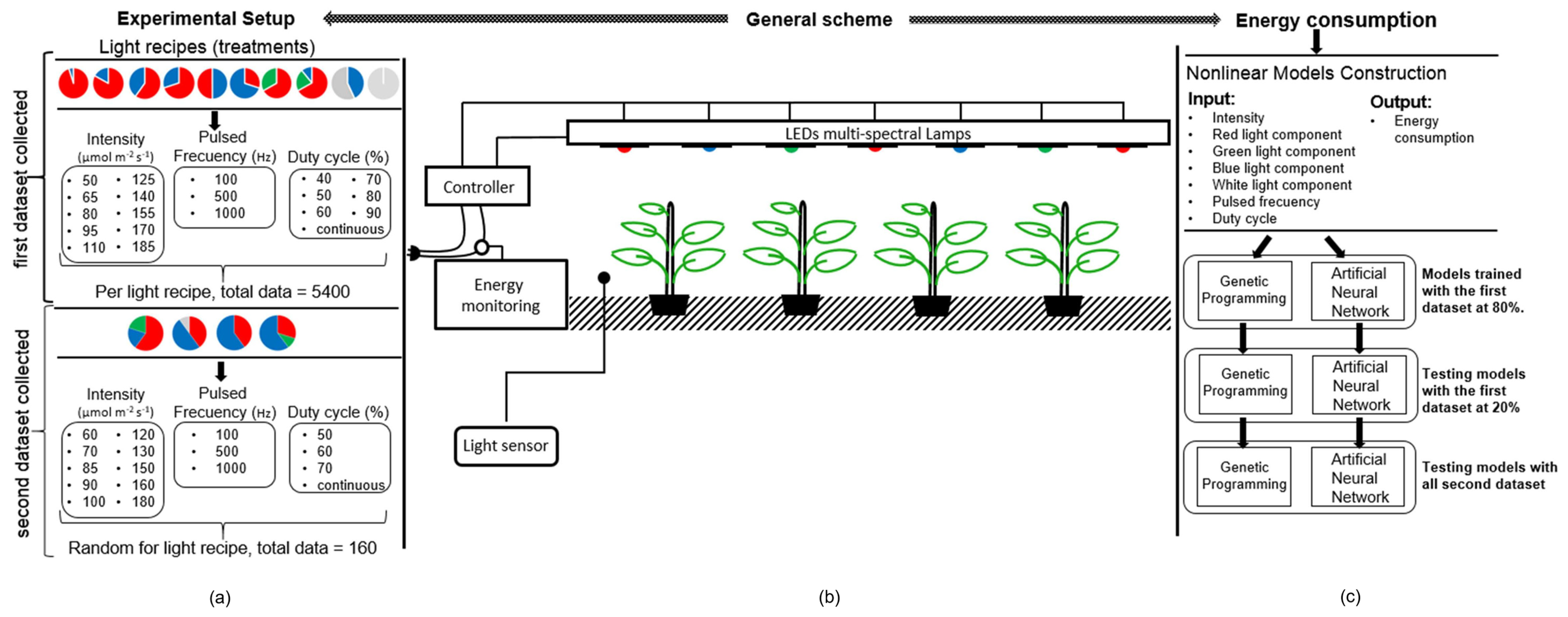
In the literature, the relationship between the spectral quality of radiation and the development and growth of crops is widely addressed. Research shows that the combination of different wavelengths can enhance the antioxidant capacity, calcium, potassium, magnesium, and phosphorus levels, number of fruits, and dry and fresh weight of vegetable crops including lettuce, spinach, kale, basil, and sweet pepper crops, among others [15,16,17]. Ten light recipes (as shown by the circles at the top of Figure 1a) in continuous and pulsed mode were used in this research to produce the first dataset (Table 1). These light recipes were selected based upon information provided in the literature. The letters in the treatments (Table 1 and Table 2) indicate the first letter of the color used (R = red, B = blue, G = green, and W = white). The intensities applied were 50, 65, 80, 95, 110, 125, 140, 155, 170, 185 µmol m−2 s−1 and the frequency was set at 100, 500, and 1000 Hz with duty cycles of 40%, 50%, 60%, 70%, 80%, 90% for each treatment (see Figure 1a). The second dataset was constructed with the design of four different light recipes (circles at the bottom of Figure 1a) at intensities of 60, 70, 85, 90, 100, 120, 130, 150, 160, 180 µmol m−2 s−1, frequencies of 100, 500, and 1000 Hz, and with randomly selected duty cycles of 60%, 70%, and 80%, as shown in Table 2. The general configuration and control of the illumination system are shown in Figure 1b. We selected the inputs and output, splitting the dataset in 80% for training and 20% for testing. The training stage fixes the algorithm’s parameters with ten-folds cross-validation to obtain the best predictions of energy consumption through the light recipes shown in Figure 1c. Triplicate experiments for all conditions were carried out with both continuous and pulsed LED light modes.

2.3. Energy Consumption

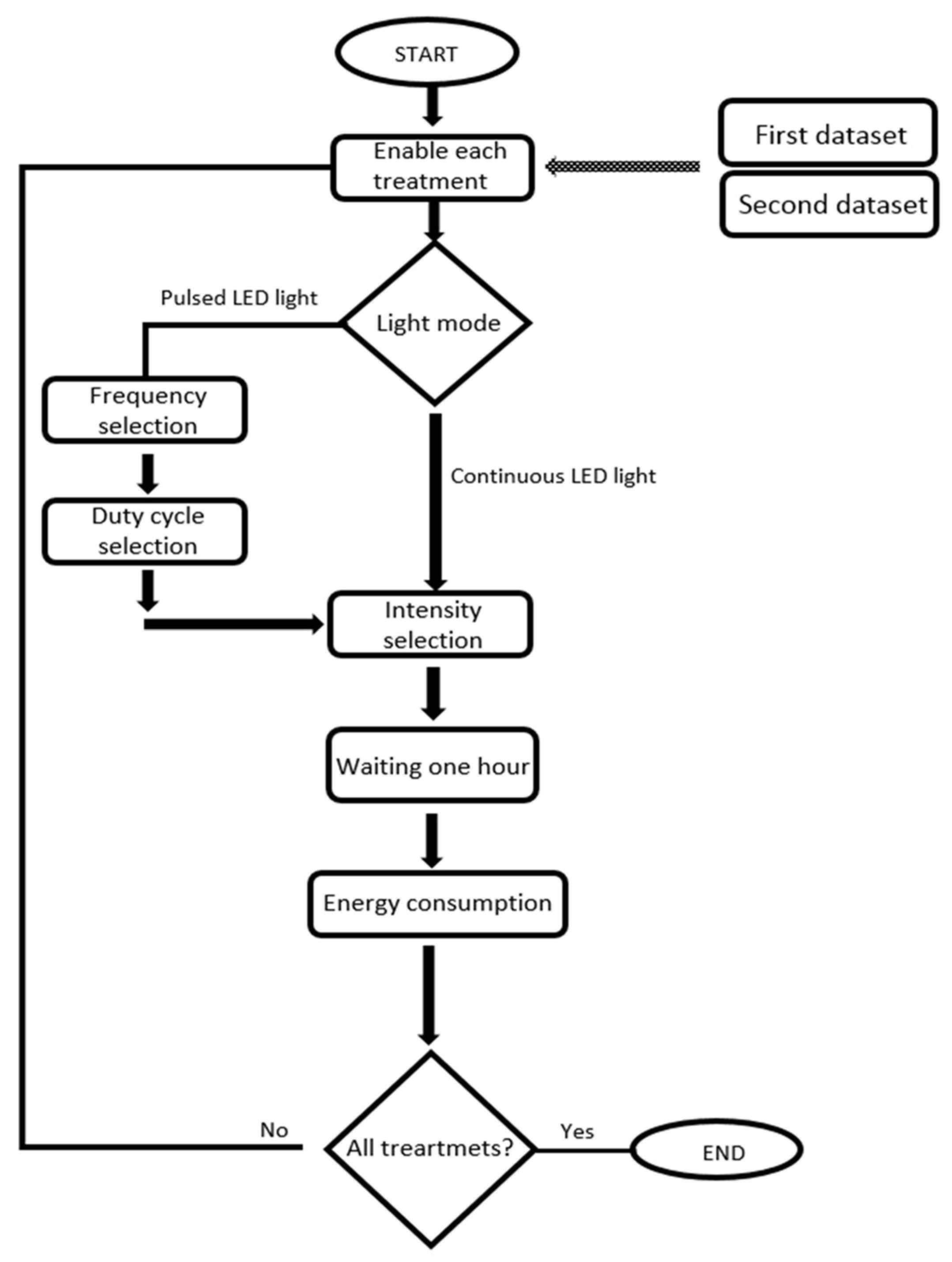
Figure 2 displays the data acquisition sequence. The artificial radiation system with each light recipe (Table 1 and Table 2) at different intensities, frequencies, and duty cycles for the two datasets was programmed as indicated in Figure 1a. For each light recipe, after 60 min of irradiation, energy consumption was measured with a hook-on AC ammeter (Peak Teach, Salerno, Italy) and was expressed in watt × hour (Wh). The reconfiguration of a new light recipe or treatment consisted of turning off the artificial radiation system for 15 min to allow it to cool down.

2.4. Nonlinear Test of Energy Consumption in Irradiation LED Lighting System

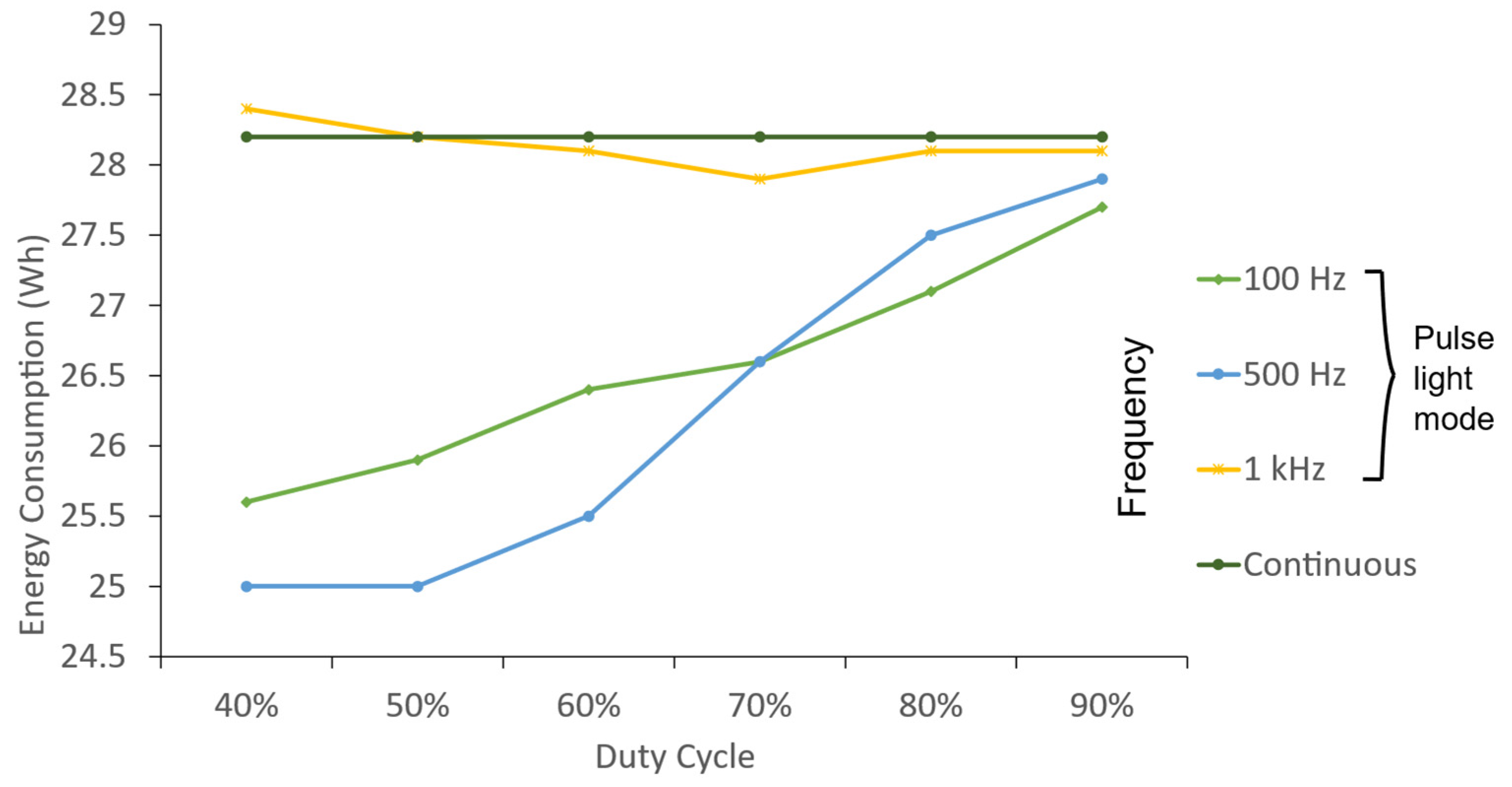
According to the process for obtaining the energy consumption measurements detailed in Figure 2, a linear transformation test (linear mapping) was applied, as described in [47], in order to prove that the obtained datasets demonstrated nonlinear behavior. Figure 3 shows the nonlinear behavior of energy consumption for the values obtained in the measurement process. The light recipe applied for this data was 95R5B at 110 µmol m−2 s−1 from Dataset 1.
We defined f as a function that maps the changes in energy consumption given by modifying the pulsed frequency (x6); then, if the model is lineal, the following equations should be satisfied: f ( x 6 = 500   Hz ) = 5   f ( x 6 = 100   Hz ) and f ( x 6 = 500   Hz ) =   f ( x 6 = 100   Hz ) + f ( x 6 = 100   Hz ) + f ( x 6 = 100   Hz ) + f ( x 6 = 100   Hz ) + f ( x 6 = 100   Hz ) . We tested linearity according to the method described in [47], with the light recipe 95R5B at 110 µmol m−2 s−1 and 80% duty cycle from the dataset 1 by considering these axioms that define a linear map.
f ( 500 ) = f ( 100 ) + f ( 100 ) + f ( 100 ) + f ( 100 ) + f ( 100 ) f ( 500 ) = 5 f ( 100 ) 0.4 5.5
The information previously presented demonstrates that there is a nonlinear phenomenon in the energy consumption behavior of the lighting system, generated by the input parameters.

2.5. Genetic Programming

Genetic programming (GP), developed by John Koza in 1992, is an evolutionary algorithm that generates unknown structures through metaheuristic optimization based on the natural selection principles proposed by Charles Darwin [36,38,48]. The linear GP variant requires fewer pointers and has candidate solutions which are compatible with programming instructions [49,50,51].
The algorithm starts with the random generation of (SP) chromosomes with (NO) operators. After that, the fitness function evaluates the quality of each chromosome (f(xL)). Then, the tournament randomly selects (ST) chromosomes for the mating pool (MP), where those with the best fitness generate offspring (O) with crossover operation, as detailed by Poli et al. [36]. Then, the offspring with probability (PM) is mutated, and two mutation points select the mutated alleles [42,44]. The algorithm runs (NG) generations and returns the best individual in the population.

2.6. Feedforward Artificial Neural Networks

Artificial neural networks (ANNs), first proposed in the 1950s, are used in regression and classification tasks [37]. Feedforward neural networks (FNNs) are ANNs that propagate signals from input to output without feedback elements [52]. The neuron output in the output layer is given by Equation (2).
a m + 1 = f m + 1 ( W m + 1 a m + b m + 1 )
where fm+1 is the activation function, W m+1 is the weight matrix, and bm+1 the bias matrix in the layer m+1, am as the previous neuron output in the layer m, and m = 0, 1…, M−1, where M represents the number of layers [52].
The fm+1 activation functions are hyperbolic tangent sigmoids (tanh) represented in Equation (3) for hidden layers. Moreover, the linear function indicated in Equation (4) provides approximations with finite discontinuities [52].
tanh (   n m i ) = 2 1 + e 2 n m i 1
l i n e a r ( n m i ) = n m i
With n m i = j = 1 s m 1 w m i , j a m 1 j + b m i , where w m i , j is the i , j element of the weight’s matrix W m, corresponding with the i neuron in the m layer and its j input; a m 1 i is the output of the neuron i at layer m 1 ; and b m i is the bias of the neuron i at layer m .
In this proposal, we train the FNNs with scaled conjugate gradient (SCG) backpropagation, which calculates the gradient in specific conjugate directions with increased convergence speed, as proposed by Moller in 1993.

2.7. Spearman’s Correlation

The feature selection simplifies a regression problem by decreasing the number of variables. A common technique for discriminating features is the Spearman correlation, which discards inputs with lower contribution to the output based on two coefficients [53,54,55]. The ρ coefficient identifies the correlation level described by Equation (5), and the Pvalue represents the correlation reliability, i.e., the probability of presenting the correlation [55].
ρ = 1 6 D 2 n ( n 2 1 )
where n is the number of samples and D is the difference between the ranks of the samples in the dataset.

2.8. Procedure for the Construction of the Nonlinear Models

The model generation starts by calculating the Spearman coefficients for the inputs related to the output. Then, the inputs that achieve the specific threshold for ρ and Pvalue are selected. Next, it is necessary to train the GP and FNNs models.
The GP algorithm applies summation (+), subtraction (−), multiplication (×), division (÷), and exponentiation (^) as operators; numerical coefficients; Intensity (x1), red light component (x2), green light component (x3), blue light component (x4), white light component (x5), pulsed frequency (x6), and duty cycle (x7) as input variables. Finally, sines and cosines of each variable are used to build Fourier series with which to approximate any function with a finite number of discontinuities [56].
The mean absolute error (MAE) in Equation (6) is the GP cost function that estimates the error magnitude in models with unknown distribution [57].
M A E ( y ^ , y ) = 1 N i = 1 N | y ^ i y i |
where y is the real output and y ^ = g ( x 1 , , x 7 ) is the model output.
Candidate solutions are refined over NG generations using M A E ( y ^ , y ) , and then the best candidate is returned.
The FNN structure is constructed according to the process described in Section 2.5, and applied to the same vector input as the GP model. For the FNN model, we used the mean square error (MSE) defined in Equation (7). The MSE is the expected error function, because it prioritizes larger reduction errors and generates a higher quantity of derivatives for updating the ANNs weights [52].
M S E ( y ^ , y ) = 1 N i = 1 N ( y ^ y ) 2
where N is the number of samples, y is the target, and y ^ as the computed output of the FNNs.
After generating both models, we carried out a quantitative evaluation with the MAE and MSE metrics in the nonlinear models, and the errors in the construction stage were applied. The precision measures in nonlinear regression models [58,59] are the standard error of the estimate (SEE) in Equation (8) and the mean absolute percentage error (MAPE) defined in Equation (9). The SEE represents the average distance from a real output value to a predicted one. The MAPE symbolizes the average relative error between the regression model and the right measure.
S E E ( y ^ , y ) = i = 1 N ( y ^ i y i ) 2 N
M A P E ( y ^ , y ) = 1 N i = 1 N | y ^ i y i y i |
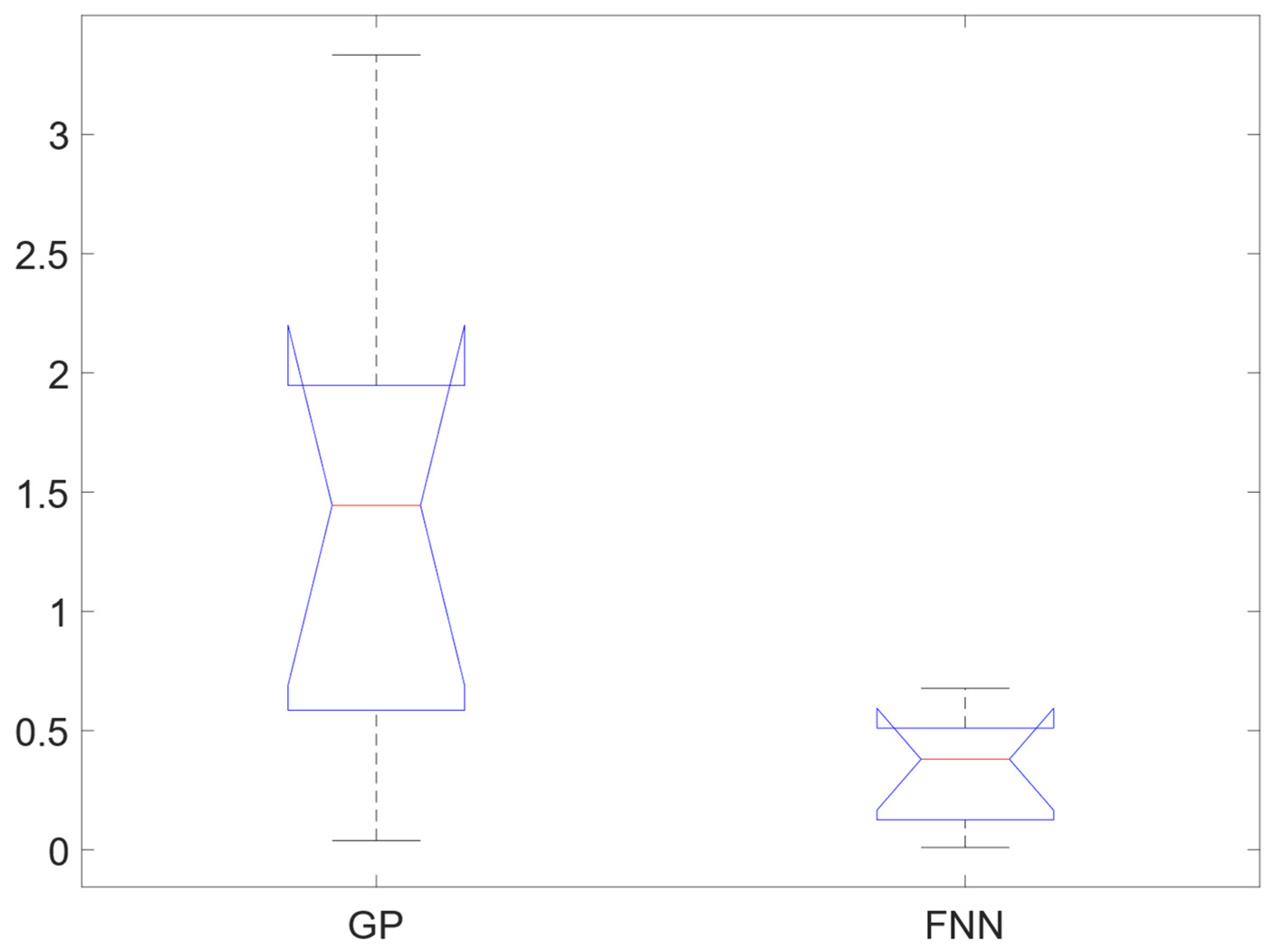
Additionally, we used three statistic validation tests to identify the best model. The first was the R2 statistic measure used in Equation (10); this is commonly used for scoring regression models, as in [60,61,62]. R2 is in the range of [0,1] with 1 for a regression model that fully explains the variability of the output variable [63]. The second is a box plot that compares, in a graphical representation, the media and quartiles of the analyzed groups. In this case, we tested the GP and FNN errors in a single dimension. The third is one-way analysis of variance (ANOVA), which was used to examine equality between two categorical variables (GP or FNN model) of quantitative outcomes with two or more levels of treatments (with metrics of error including MAE, MSE, SEE, and MAPE) [64].
R 2 ( y ^ , y , y ¯ ) = i = 1 N ( y i y ¯ ) 2 i = 1 N ( y i y ^ i ) 2 i = 1 N ( y i y ^ i ) 2

3. Results and Discussion

Two datasets for the generation and testing the GP and FNNs were applied. The first (Test 1) has 5700 samples with similar input ranges for training and evaluation; the second (Test 2) included a total of 160 datapoints in different input ranges from those used for training. The two models used energy consumption as output, while the inputs were intensity, red light component, blue light component, green light component, white light component, pulsed Frequency, and duty Cycle.
We normalized the first dataset to get its variables on the same scale. Table 3 presents the slopes and offsets for normalization. Subsequently, the most relevant inputs in Test 1 were selected if Spearman’s p value < 0.05 and ρ ≥ 0.05, which implied a weak correlation with 95% reliability [59]. Table 4 shows the correlation coefficients obtained using the inputs indicated in bold. After that, we split Test 1 as follows: 80% for the training and 20% for testing; meanwhile, Test 2 was also applied for testing in both models.
All the training stages for the GP and FNN models of this work were performed without parallel computing on a computer with Microsoft Windows 10.0.19041 Pro OS, Intel Core™ i7-6700 CPU with 3.40GHz, 16 GB RAM, and NVIDIA GeForce GTX 970 graphic card.
The GP training parameters selected with cross-validation were: SP = 200, ST = 20, and PM = 8%, for a limit of NG = 5000 generations. We avoided overfitting by selecting the complexity parameters (number of operations per parentheses and the number of parentheses) with 10-fold cross-validation in the training set. The best parameters obtained were 16 operators and 2 parentheses, with a cross-validation MAE of 3.0649, after testing 1−20 operators and 1−2 parentheses.
The GP model in the Equation (11) omitted input three (green light component), according to Spearman’s correlations in Table 2.
g ( x 1 , x 2 , x 3 , x 4 , x 5 , x 6 , x 7 ) = sin ( x 1 ) 3 2 cos ( x 1 ) cos ( x 6 ) sin ( x 5 ) 7 x 2 cos ( x 7 ) + x 6 5 + 8 x 5 + 6 x 6 + cos ( x 2 ) sin ( x 4 ) + cos ( x 7 ) sin ( x 7 ) + 7 sin ( x 1 ) x 7 sin ( x 4 ) 3 9 x 4 cos ( x 7 ) sin ( x 4 ) + 7
We selected the complexity parameters of the FNNs model with 10-fold cross-validation obtaining three layers and 10 neurons per layer after testing 1–5 layers and 1–10 neurons, with a cross-validated MSE of 0.8666, and took 21,829.51 s or 6.06 h.

3.1. GP and FNNs Behavior in Test 1

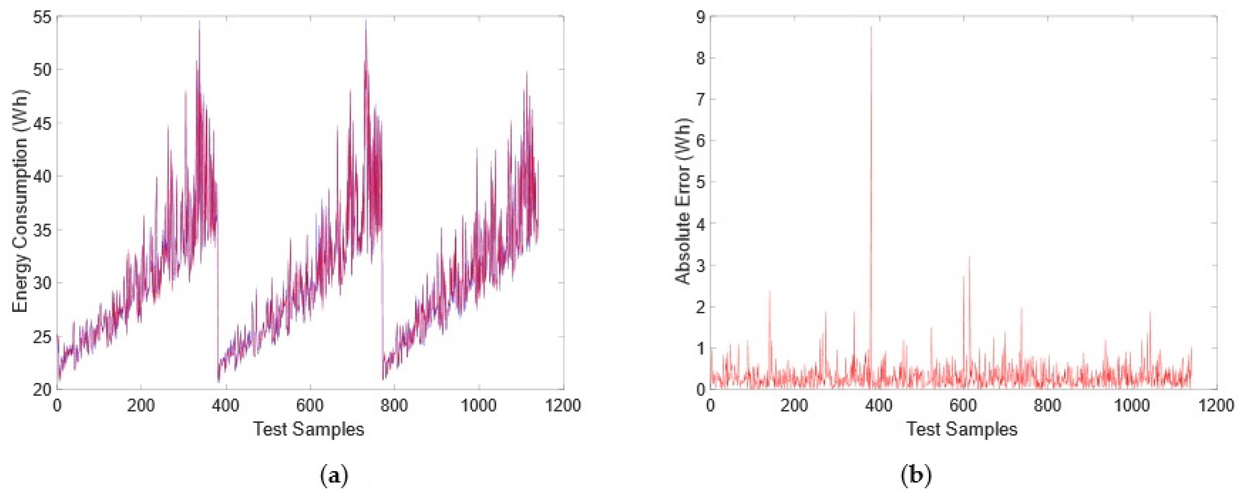
The metrics for Test 1 with similar ranges to the training showed (Table 5) that the GP model achieved 96.1% precision (1-MAPE), 3.90% MAPE, an average error between a real output value and a predicted one of 1.4384 watts (SEE), and 92.67% effectiveness at explaining the variability of the output variable (R2). The MAE estimated for the GP model was 1.1239 and 3.0649 in the testing stage for the cross-validated MAE, i.e., a cross-validated error which was higher than the test error, which indicated a model without overfitting. In this context, the FNNs model obtained an accuracy or 1-MAPE, a MAPE, and the average errors between the real output value and a predicted one were 98.99%, 1.01%, and 0.4827 watts (SEE), respectively. The FNNs model effectively explains 99.34% of the variability of the output variable (R2). The MSE for the ANN model was 0.3007 and 0.8666 in the testing stage for the cross-validated MSE, i.e., a cross-validated error higher than the test error, which indicated a model without overfitting.
Furthermore, FNNs showed slightly better performance than GP in the testing stage. The MAE and MSE levels were lower in FNNs, despite the training measures, as indicated in Table 5.
The GP model response (red line) and the desired output (blue line) are shown in Figure 4a. The absolute error (AE) is plotted in Figure 4b to identify the highest error per sample, i.e., 7 watts compared to 1.1239 watts of MAE.
The FNNs model response (Figure 5a) exhibited a higher accuracy than the GP model, with finding a lower MAE, i.e., 0.3007, but a bigger punctual error that reached almost 9 watts (Figure 5b).

3.2. GP and FNNs Models Behavior in Test 2

The accuracy metrics of Test 2 with different ranges to those used for training are shown in Table 6. The GP model reached 95.35% accuracy, 4.65% error (MAPE); its average error (SEE) from a real output value to a predicted one was 1.8256 watts, which explains 83.99% of output variability (R2). The FNNs model achieved 98.21% accuracy (1-MAPE) and 1.79% error (MAPE); the average error (SEE) between a real output value and a predicted one was 0.6776 watts, which explains 97.79% of the output variability (R2).
The two datasets (Test 1 and Test 2) showed that the FNNs model was slightly superior to the GP model in the testing stage, despite the training measures. As shown in Table 6, the error levels for MAE and MSE were lower in FNNs, while their effectiveness explaining the variable output variability or R2 was superior.
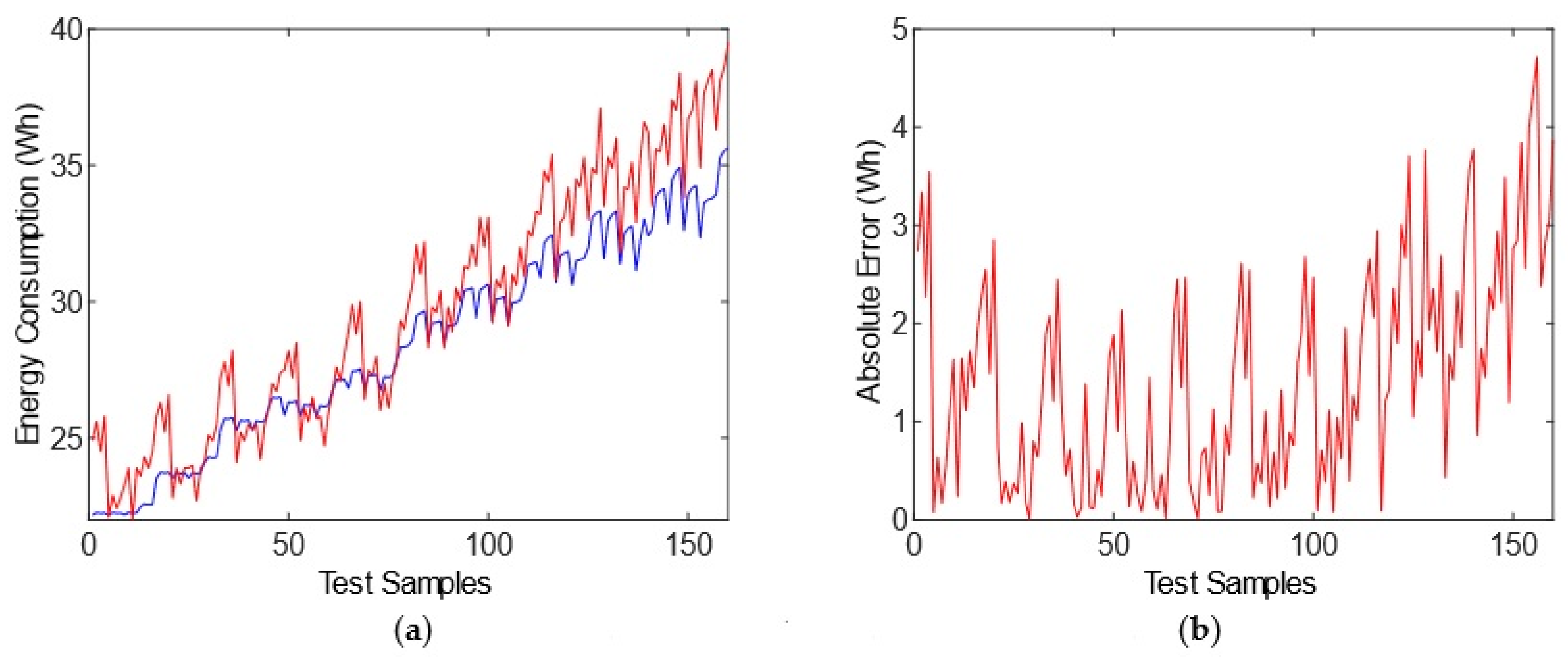
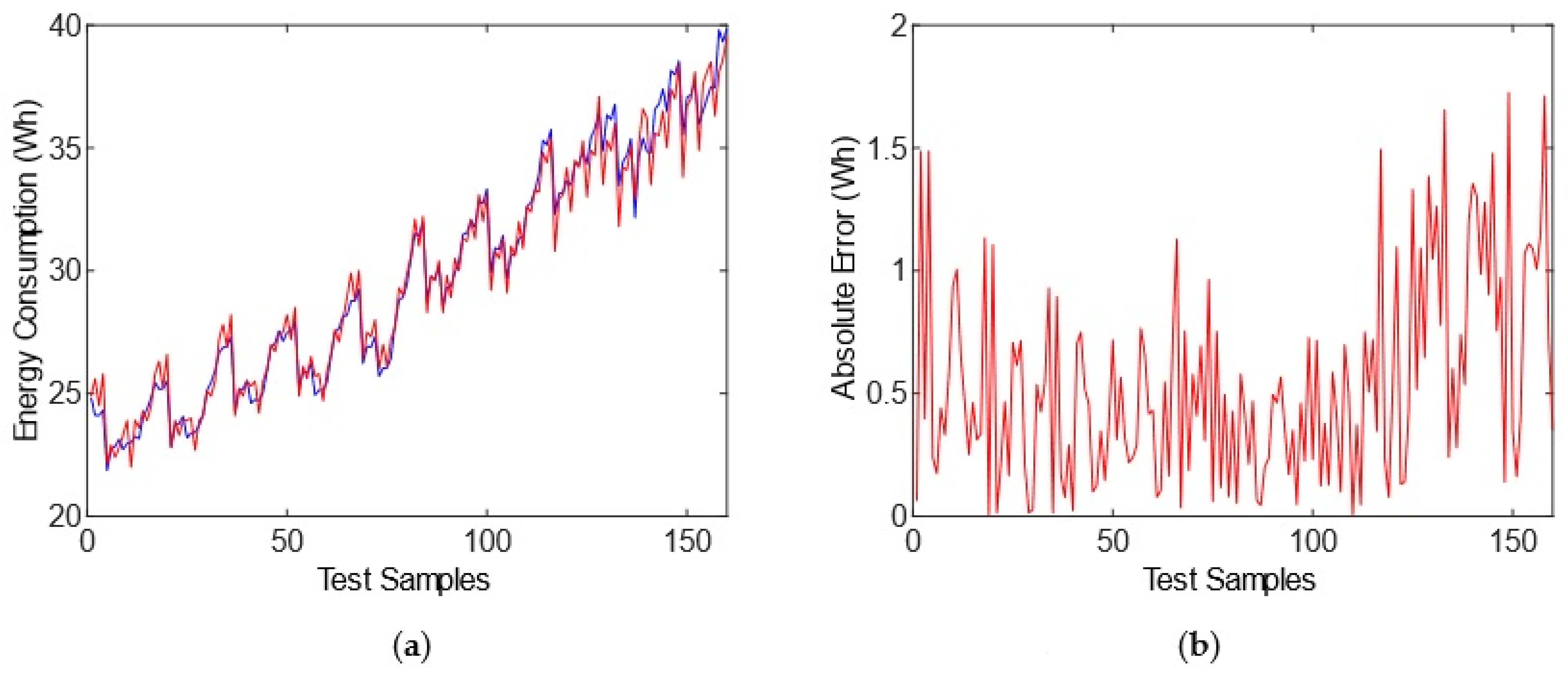
A comparative response between the obtained GP model output and the desired one (red and blue signals, respectively) is shown in Figure 6a. We plotted AE in Figure 6b, showing a maximum error per sample of 4.6 watts, despite a MAE of 1.4508. The FNNs model response (Figure 7a) exhibited a higher accuracy than the GP model, with a lower MAE of 0.5386, and presented a lower punctual error than the GP model, i.e., almost 1.8 watts (Figure 7b).

3.3. GP and FNNs Models Statistic Comparison

The estimated errors (MAE, MSE, SEE, and MAPE) for each nonlinear model (GP model and FNNs) in Tests 1 and 2 were integrated and associated with a new group of analyses (box plot and ANOVA). According to results obtained in the ANOVA and the graphic (box plot), it was determined that the FNNs model showed the best performance, considering the error and variance values, as observed in Figure 8. Furthermore, the ANOVA with P v a l u e = 0.0155 supports these results, given that the established hypothesis (the error FNN < GP) is true with a 1.55% risk (Table 7).

4. Conclusions

In this proposal, we compared two nonlinear models for predicting energy consumption in CPPS using a linear GP algorithm and FNNs. The models generated energy consumption as output, and took intensity, red light component, blue light component, green light component, white light component, pulsed frequency, and duty cycle as input variables.
We identified the most important variables with Spearman’s correlation. The accuracy achieved using similar test ranges to those used in training was 96.1% for the GP model and 98.99% for the FNNs. On the other hand, the accuracy achieved with different test ranges to those used in training was 95.35% for GP and 98.21% for FNNs. Test 2 indicated that FNNs had better generalization than GP.
We found that the FNNs model was superior to the GP model based on statistical tests R2, box plot, and one-way ANOVA with a risk probability of 1.55%. Additionally, FNNs trained faster (6.063 h), in terms of processing all the tested architectures, than GP, which required 169.274 h due to the high computational cost, as noted in the literature.
The GP and FNNs models generated in this proposal can be applied or programmed as part of a monitoring system for CPPS which prioritize energy efficiency. The results showed that the models achieved a forecast of energy consumption through a detailed analysis with each of the input variables. In this way, any new light recipe introduced in the literature or generated by the user generates a prediction about energy consumption. Projections of energy consumption are performed offline by moving the input parameters for both light operation modes (continuous and pulsed). The evaluation offered an advantage in several applications, as the pulsed light demonstrated energy savings through the application of different pulsed frequencies and duty cycles, compared with the continuous light. The proposed nonlinear models are directly connected to energy consumption predictions in real artificial radiation systems, so nonlinearities and parametric uncertainties were considered in the analysis. However, using new artificial lighting systems in CPPS implies retraining the model. However, once the models that describe the behavior of a lighting system have been trained, similar modules can be applied to cover a larger irradiation area without requiring remodeling. The proposed methodology serves as a reference for researchers, technicians, specialists, and entrepreneurs within the agro-industrial sector.
Author Contributions

All authors conceived the experiments, E.O.-G., N.E.-G. and E.F.-G. recollected the data for the experiments, M.M.R. and E.O.-G. conducted the experiments, performed statistical analysis, and figure generation. All authors wrote and reviewed the manuscript. All authors have read and agreed to the published version of the manuscript.

Funding

We acknowledge the support of the Consejo Nacional de Ciencia y Tecnología (CONACYT) in Mexico for supporting this work through funds for projects INFRA-2016-01, Project No. 270665. CB-2016-01, Project No. 287828.

Institutional Review Board Statement

Not applicable.

Informed Consent Statement

Not applicable.

Data Availability Statement

Not applicable.

Conflicts of Interest

The authors declare no conflict of interest.

References

  1. Benke, K.; Tomkins, B. Future food-production systems: Vertical farming and controlled-environment agriculture. Sustain. Sci. Pract. Policy 2017, 13, 13–26. [Google Scholar] [CrossRef] [Green Version]
  2. Eaves, J.; Eaves, S. Comparing the profitability of a greenhouse to a vertical farm in Quebec. Can. J. Agric. Econ. 2018, 66, 43–54. [Google Scholar] [CrossRef]
  3. Kalantari, F.; Tahir, O.M.; Lahijani, A.M.; Kalantari, S. A review of vertical farming technology: A guide for implementation of building integrated agriculture in cities. Adv. Eng. Forum 2017, 24, 76–91. [Google Scholar] [CrossRef]
  4. Rabara, R.C.; Behrman, G.; Timbol, T.; Rushton, P.J. Effect of spectral quality of monochromatic LED lights on the growth of artichoke seedlings. Front. Plant Sci. 2017, 8, 190. [Google Scholar] [CrossRef] [Green Version]
  5. Ata, K.; Urano, M.; Takahashi, A. Thermal analysis of pulsed LED lighting in Plant Factory. In Proceedings of the IMFEDK 2017—2017 International Meeting for Future of Electron Devices, Kansai, Japan, 29–30 June 2017; pp. 56–57. [Google Scholar]
  6. Kozai, T. Smart plant factory: The next generation indoor vertical farms. In Plant Factories with Artificial Lighting (PFALs): Benefits, Problems and Challenges; Springer: Singapore, 2018; pp. 15–29. ISBN 978-981-13-1064-5. [Google Scholar]
  7. Kozai, T.; Fujiwara, K.; Runkle, E.S. LED Lighting for Urban Agriculture, 1st ed.; Springer: Berlin/Heidelberg, Germany, 2016; ISBN 9789811018480. [Google Scholar]
  8. Shimizu, H.; Saito, Y.; Nakashima, H.; Miyasaka, J.; Ohdoi, K. Light environment optimization for lettuce growth in plant factory. In Proceedings of the 18th IFAC World Congress, Milano, Italy, 28 August–2 September 2011; pp. 605–609. [Google Scholar]
  9. Son, K.H.; Jeon, Y.M.; Oh, M.M. Application of supplementary white and pulsed light-emitting diodes to lettuce grown in a plant factory with artificial lighting. Hortic. Environ. Biotechnol. 2016, 57, 560–572. [Google Scholar] [CrossRef]
  10. Germer, J.; Sauerborn, J.; Asch, F.; de Boer, J.; Schreiber, J.; Weber, G.; Müller, J. Skyfarming an ecological innovation to enhance global food security. J. Fur Verbraucherschutz Und Leb. 2011, 6, 237–251. [Google Scholar] [CrossRef]
  11. Kalantari, F.; Tahir, O.M.; Joni, R.A.; Fatemi, E. Opportunities and challenges in sustainability of vertical farming: A review. J. Landsc. Ecol. Repub. 2018, 11, 35–60. [Google Scholar] [CrossRef] [Green Version]
  12. Schubert, E.F.; Kim, J.K. Solid-state light sources getting smart. Science 2005, 308, 1274–1278. [Google Scholar] [CrossRef] [PubMed]
  13. Bian, Z.H.; Cheng, R.F.; Yang, Q.C.; Wang, J.; Lu, C. Continuous light from red, blue, and green light-emitting diodes reduces nitrate content and enhances phytochemical concentrations and antioxidant capacity in lettuce. J. Am. Soc. Hortic. Sci. 2016, 141, 186–195. [Google Scholar] [CrossRef] [Green Version]
  14. Gupta, S.D.; Agarwal, A. Artificial lighting system for plant growth and development: Chronological advancement, working principles, and comparative assessment. In Light Emitting Diodes for Agriculture: Smart Lighting, 1st ed.; Springer: Berlin/Heidelberg, Germany, 2017; pp. 1–25. ISBN 9789811058073. [Google Scholar]
  15. Meng, Q.; Kelly, N.; Runkle, E.S. Substituting green or far-red radiation for blue radiation induces shade avoidance and promotes growth in lettuce and kale. Environ. Exp. Bot. 2019, 162, 383–391. [Google Scholar] [CrossRef]
  16. Mickens, M.A.; Skoog, E.J.; Reese, L.E.; Barnwell, P.L.; Spencer, L.E.; Massa, G.D.; Wheeler, R.M. A strategic approach for investigating light recipes for ’Outredgeous’ red romaine lettuce using white and monochromatic LEDs. Life Sci. Sp. Res. 2018, 19, 53–62. [Google Scholar] [CrossRef] [PubMed]
  17. Naznin, M.T.; Lefsrud, M.; Gravel, V.; Azad, M.O.K. Blue light added with red LEDs enhance growth characteristics, pigments content, and antioxidant capacity in lettuce, Spinach, Kale, Basil, and sweet pepper in a controlled environment. Plants 2019, 8, 93. [Google Scholar] [CrossRef] [Green Version]
  18. Ahmed, H.A.; Yu-Xin, T.; Qi-Chang, Y. Optimal control of environmental conditions affecting lettuce plant growth in a controlled environment with artificial lighting: A review. S. Afr. J. Bot. 2020, 130, 75–89. [Google Scholar] [CrossRef]
  19. Zeidler, C.; Schubert, D. From bioregenerative life support systems for space to vertical farming on earth—The 100% spin-off. In Proceedings of the Life in Space for Life on Earth Symposium, Waterloo, ON, Canada, 15–20 June 2015. [Google Scholar]
  20. Watanabe, H. Light-controlled plant cultivation system in Japan—Development of a vegetable factory using LEDs as a light source for plants. Acta Hortic. 2011, 907, 37–44. [Google Scholar] [CrossRef]
  21. Watson, R.T.; Boudreau, M.-C.; van Iersel, M.W. Simulation of greenhouse energy use: An application of energy informatics. Energy Inform. 2018, 1, 1. [Google Scholar] [CrossRef] [Green Version]
  22. Hwang, P.W.; Chen, C.H.; Chang, Y.J. A study on energy strategy of a plant factory using sustainable energy combined with computational fluid dynamics simulation: An innovative practice of green information systems. In Proceedings of the 2017 Computing Conference, London, UK, 18–20 July 2017; pp. 517–522. [Google Scholar]
  23. Sørensen, J.C.; Kjaer, K.H.; Ottosen, C.O.; Jørgensen, B.N. DynaGrow—Multi-objective optimization for energy cost-efficient control of supplemental light in greenhouses. In Proceedings of the 8th International Joint Conference on Computational Intelligence, Porto, Portugal, 9–11 November 2016; pp. 41–48. [Google Scholar]
  24. Cheng, Y. Research on intelligent control of an agricultural greenhouse based on fuzzy PID control. J. Environ. Eng. Sci. 2020, 15, 113–118. [Google Scholar] [CrossRef]
  25. Gouadria, F.; Sbita, L.; Sigrimis, N. Comparison between self-tuning fuzzy PID and classic PID controllers for greenhouse system. In Proceedings of the International Conference on Green Energy and Conversion Systems (GECS), Hammamet, Tunisia, 23–25 March 2017; pp. 23–25. [Google Scholar]
  26. Hamza, A.; Ramdani, M. Non-PDC interval type-2 fuzzy model predictive microclimate control of a greenhouse. J. Control. Autom. Electr. Syst. 2020, 31, 62–72. [Google Scholar] [CrossRef]
  27. Singh, V.K.; Tiwari, K.N. Prediction of greenhouse micro-climate using artificial neural network. Appl. Ecol. Environ. Res. 2017, 15, 767–778. [Google Scholar] [CrossRef]
  28. Francik, S.; Kurpaska, S. The use of artificial neural networks for forecasting of air temperature inside a heated foil tunnel. Sensors 2020, 20, 652. [Google Scholar] [CrossRef] [Green Version]
  29. Jung, D.H.; Kim, H.S.; Jhin, C.; Kim, H.J.; Park, S.H. Time-serial analysis of deep neural network models for prediction of climatic conditions inside a greenhouse. Comput. Electron. Agric. 2020, 173, 105402. [Google Scholar] [CrossRef]
  30. Escamilla-García, A.; Soto-Zarazúa, G.M.; Toledano-Ayala, M.; Rivas-Araiza, E.; Gastélum-Barrios, A. Applications of artificial neural networks in greenhouse technology and overview for smart agriculture development. Appl. Sci. 2020, 10, 3835. [Google Scholar] [CrossRef]
  31. Gros, S.; Zanon, M.; Quirynen, R.; Bemporad, A.; Diehl, M. From linear to nonlinear MPC: Bridging the gap via the real-time iteration. Int. J. Control 2020, 93, 62–80. [Google Scholar] [CrossRef]
  32. Ouammi, A.; Achour, Y.; Zejli, D.; Dagdougui, H. Supervisory model predictive control for optimal energy management of networked smart greenhouses integrated microgrid. IEEE Trans. Autom. Sci. Eng. 2020, 17, 117–128. [Google Scholar] [CrossRef]
  33. Xu, H.; Zhai, Z.; Wang, K.; Ren, S.; Wang, H. Multiobjective distributed model predictive control method for facility environment control based on cooperative game theory. Turk. J. Electr. Eng. Comput. Sci. 2017, 25, 4160–4171. [Google Scholar] [CrossRef]
  34. Lin, D.; Zhang, L.; Xia, X. Hierarchical model predictive control of Venlo-type greenhouse climate for improving energy efficiency and reducing operating cost. J. Clean. Prod. 2020, 264, 121513. [Google Scholar] [CrossRef]
  35. Montes Rivera, M.; Paz Ramos, M.; Orozco Mora, J. Automatic generator of decoupling blocks using genetic programming. In New Trends in Networking, Computing, E-Learning, Systems Sciences, and Engineering; Springer: Berlin/Heidelberg, Germany, 2015; pp. 281–290. ISBN 978-3-319-06764-3. [Google Scholar]
  36. Poli, R.; Langdon, W.B.; McPhee, N.F.; Koza, J.R. A field guide to Genetic Programming; Lulu Press: London, UK, 2008; ISBN 978-1409200734. [Google Scholar]
  37. Goodfellow, I.; Bengio, Y.; Courville, A. Deep Learning; The MIT Press: Cambridge, UK, 2016; ISBN 0262035618/978-0262035613. [Google Scholar]
  38. Brameier, M.; Banzhaf, W. A comparison of linear genetic programming and neural networks in medical data mining. IEEE Trans. Evol. Comput. 2001. [Google Scholar] [CrossRef] [Green Version]
  39. Kobashigawa, J.; Youn, H.S.; Iskander, M.; Yun, Z. Comparative study of genetic programming vs. neural networks for the classification of buried objects. In Proceedings of the IEEE Antennas and Propagation Society, AP-S International Symposium (Digest), North Charleston, SC, USA, 1–5 June 2009; pp. 1–4. [Google Scholar]
  40. Fatehnia, M.; Amirinia, G. A review of Genetic Programming and Artificial Neural Network applications in pile foundations. Int. J. Geo-Eng. 2018, 9. [Google Scholar] [CrossRef] [Green Version]
  41. Can, B.; Heavey, C. A comparison of genetic programming and artificial neural networks in metamodeling of discrete-event simulation models. Comput. Oper. Res. 2012, 39, 424–436. [Google Scholar] [CrossRef]
  42. Berrar, D. Cross-validation. In Encyclopedia of Bioinformatics and Computational Biology: ABC of Bioinformatics; Elsevier: Amsterdam, The Netherlands, 2018; Volume 1–3, pp. 542–545. ISBN 9780128114322. [Google Scholar]
  43. Grimm, K.J.; Mazza, G.L.; Davoudzadeh, P. Model Selection in Finite Mixture Models: A k-Fold Cross-Validation Approach. Struct. Equ. Model. 2017, 24, 246–256. [Google Scholar] [CrossRef]
  44. Jung, K.; Bae, D.H.; Um, M.J.; Kim, S.; Jeon, S.; Park, D. Evaluation of nitrate load estimations using neural networks and canonical correlation analysis with K-fold cross-validation. Sustainability 2020, 12, 400. [Google Scholar] [CrossRef] [Green Version]
  45. Fang, L.; Liu, S.; Huang, Z. Uncertain Johnson–Schumacher growth model with imprecise observations and k-fold cross-validation test. Soft Comput. 2020, 24, 2715–2720. [Google Scholar] [CrossRef]
  46. Xiong, Z.; Cui, Y.; Liu, Z.; Zhao, Y.; Hu, M.; Hu, J. Evaluating explorative prediction power of machine learning algorithms for materials discovery using k -fold forward cross-validation. Comput. Mater. Sci. 2020, 171, 109203. [Google Scholar] [CrossRef]
  47. Pavan, V. Reminders on Linear Algebra. In Exterior Algebras; Elsevier: Amsterdam, The Netherlands, 2017; pp. 1–18. [Google Scholar]
  48. Olmo, J.L.; Romero, J.R.; Ventura, S. Swarm-based metaheuristics in automatic programming: A survey. Wiley Interdiscip. Rev. Data Min. Knowl. Discov. 2014, 4, 445–469. [Google Scholar] [CrossRef]
  49. Montes Rivera, M.; Aguilar Justo, M.O.; Zezzatti, A.O. Equations for describing behavior tables in thermodynamics using genetic programming: Synthesizing the saturated water and steam table. Res. Comput. Sci. 2016, 1, 9–23. [Google Scholar] [CrossRef]
  50. Brameier, M.F.; Banzhaf, W. Linear Genetic Programming (Genetic and Evolutionary Computation); Springer: New York, NY, USA, 2007; ISBN 978-0387310299. [Google Scholar]
  51. Weise, T. Global Optimization Algorithms-Theory and Application, 2nd ed.; Self-Published: 2009; Available online: http://www.it-weise.de/projects/book.pdf (accessed on 10 March 2021).
  52. Hagan, M.T.; Demuth, H.B.; Beale, M.H.; De Jesús, O. Neural Network Design, 2nd ed.; Self-Published: 1996; ISBN 978-0971732117. Available online: http://hagan.okstate.edu/nnd.html (accessed on 10 March 2021).
  53. Duan, Y.; Song, C. Relevant modes selection method based on Spearman correlation coefficient for laser signal denoising using empirical mode decomposition. Opt. Rev. 2016, 23, 936–949. [Google Scholar] [CrossRef]
  54. Broughman, J.R.; Basak, R.; Nielsen, M.E.; Reeve, B.B.; Usinger, D.S.; Spearman, K.C.; Godley, P.A.; Chen, R.C. Prostate cancer patient characteristics associated with a strong preference to preserve sexual function and receipt of active surveillance. J. Natl. Cancer Inst. 2018, 110, 420–425. [Google Scholar] [CrossRef] [Green Version]
  55. Rasch, D. Gibbons, J. D.: Nonparametric Statistical Inference, 2nd. Ed. Statistics: Textbooks and monographs vol. 65. Marcel Dekker, Inc., New York and Basel 1985, XV, 408 S., $ 41,25 ($ 34,50 US and Canada). Biom. J. 1986, 28, 936. [Google Scholar] [CrossRef]
  56. Zhang, Q.H.; Chen, S.; Qu, Y. Corrected Fourier series and its application to function approximation. Int. J. Math. Math. Sci. 2005, 2005, 33–42. [Google Scholar] [CrossRef] [Green Version]
  57. Chai, T.; Draxler, R.R. Root mean square error (RMSE) or mean absolute error (MAE)?- Arguments against avoiding RMSE in the literature. Geosci. Model Dev. 2014, 7, 1247–1250. [Google Scholar] [CrossRef] [Green Version]
  58. Smith, G. Multiple regression. In Essential Statistics, Regression, and Econometrics; Elsevier: Amsterdam, The Netherlands, 2015; pp. 301–337. [Google Scholar]
  59. De Myttenaere, A.; Golden, B.; Le Grand, B.; Rossi, F. Mean Absolute Percentage Error for regression models. Neurocomputing 2016, 192, 38–48. [Google Scholar] [CrossRef] [Green Version]
  60. Cheng, Z.L.; Zhou, W.H.; Garg, A. Genetic programming model for estimating soil suction in shallow soil layers in the vicinity of a tree. Eng. Geol. 2020, 268, 105506. [Google Scholar] [CrossRef]
  61. Jafari, H.; Rajaee, T.; Kisi, O. Improved water quality prediction with hybrid wavelet-genetic programming model and shannon entropy. Nat. Resour. Res. 2020, 29, 3819–3840. [Google Scholar] [CrossRef]
  62. De Giorgi, M.G.; Quarta, M. Hybrid MultiGene Genetic Programming—Artificial neural networks approach for dynamic performance prediction of an aeroengine. Aerosp. Sci. Technol. 2020, 103. [Google Scholar] [CrossRef]
  63. Bruce, P.; Bruce, A. Practical Statistics for Data Scientists; O’Reilly Media: Sebastopol, CA, USA, 2017; ISBN 978-1-491-95296-2. [Google Scholar]
  64. Seltman, H.J. One-way ANOVA. In Experimental Design and Analysis; Carnegie Mellon University: Pittsburgh, PA, USA, 2012; pp. 171–190. [Google Scholar]
Figure 1. General experimental design. (a) Experimental setup for the two datasets. (b) Measuring general scheme. (c) Energy consumption nonlinear models construction.
Applsci 11 02735 g001
Figure 2. Detailed procedure for data collection.
Applsci 11 02735 g002
Figure 3. Energy consumption behavior for 95R5B light recipe at 110 µmol m−2 s−1 with different pulsed frequencies and duty cycles.
Applsci 11 02735 g003
Figure 4. GP model results in Test 1. (a) Data estimated (red) versus energy consumption data measured (blue). (b) Absolute error between estimated behavior and measured energy consumption (red).
Applsci 11 02735 g004
Figure 5. FNNs model results in Test 1. (a) Data estimated (red) versus energy consumption data measured (blue). (b) Absolute error between estimated behavior and measured energy consumption (red).
Applsci 11 02735 g005
Figure 6. GP model results in Test 2. (a) Data estimated (red) versus energy consumption data measured (blue). (b) Absolute error between estimated behavior and measured energy consumption (red).
Applsci 11 02735 g006
Figure 7. FNNs model results in Test 2. (a) Data estimated (red) versus energy consumption data measured (blue). (b) Absolute error between estimated behavior and measured energy consumption (red).
Applsci 11 02735 g007
Figure 8. ANOVA comparison of error in groups GP and FNN models.
Applsci 11 02735 g008
Table 1. Light treatments (recipes) for the first dataset (Test 1).
RecipesRedGreenBlueWhite
95R5B95%0%5%0%
83R17B83%0%17%0%
60R40B60%0%40%0%
57W43B0%0%43%57%
67R11B22G67%22%11%0%
67R33G67%33%0%0%
100W0%0%0%100%
50R50B50%0%50%0%
70R30B70%0%30%0%
30R70B30%0%70%0%
Table 2. Light treatments (recipes) for the second dataset (Test 2).
RecipesRedGreenBlueWhite
60R20G20B60%20%20%0%
40R50B10W40%0%50%10%
40R60B40%0%60%0%
30R10G60B30%10%60%0%
Table 3. Slope and Offset normalization coefficients per variable.
Variables x 1 x 2 x 3 x 4 x 5 x 6 x 7 y
Slopes135.0175.7561.05129.5185.01000.090.034.10
Offsets50.0000000.020.60
Table 4. Input variables selected based on Spearman’s coefficients.
Variables x 1 x 2 x 3 x 4 x 5 x 6 x 7
ρ 0.91090.2039−0.02190.29080.30640.08910.0620
p v a l u e 000.09900000
Table 5. Models efficiency metrics for Test 1.
TechniqueMAEMSESEEMAPER2
GP1.12392.06911.43840.03900.9267
FNNs0.30070.23300.48270.01010.9934
Table 6. Models efficiency metrics for Test 2.
TechniqueMAEMSESEEMAPER2
GP1.45083.33281.82560.04650.8399
FNNs0.53860.45910.67760.01790.9779
Table 7. ANOVA analysis of error metrics MAE, MSE, SEE and MAPE between GP and FNN models for PROB > F( P v a l u e for testing null hypotesis).
Source of VariationSums of SQUARESDegree of FreedomMean Square ErrorFPROB > F
Columns4.629414.629387.590.0155
Error8.5407140.61005
Total13.170115
Publisher’s Note: MDPI stays neutral with regard to jurisdictional claims in published maps and institutional affiliations.